A framework to estimate national biofuel potential by siting production facilities: a case study for canola sustainable aviation fuel in Canada

Abstract

International Civil Aviation Organization member states need to develop national strategies for sustainable aviation fuel (SAF) production to reduce greenhouse gas emissions from aviation. In this work, we developed a framework to estimate the national SAF potential and applied it to a case study for canola SAF in Canada. Specifically, we answered (i) how many SAF plants can be constructed and what are their maximum name-plate capacities? (ii) which geographic locations can economically support a SAF plant? (iii) what could be the average life cycle GHG emissions of SAF supplied to major airports? Our study developed an improved framework for estimating the SAF potential for a region by incorporating detailed site selection criteria for identifying optimal locations. We found that 15.2 million metric tonnes (MT) of potentially available canola can supply about 1–1.8 billion litres of SAF by 2030 (12–21% of Canada's 2019 jet fuel consumption) across 7–11 optimal sites, after accounting for infrastructure and accepted industry/financing guidelines on feedstock utilization. Up to 20% of this potential is lost if there is a lack of coordination and plants are sited sequentially based on profitability instead of maximizing feedstock utilization. The life cycle-GHG emissions of the SAF produced in the optimal sites ranged between 20–58 g CO₂e per MJ, depending on the local farming practices and legacy land use & land management changes. Increasing the supply chain transportation connectivity and managing feedstock competition could provide access to more canola for SAF production; however, other pathways will also be required to meet the growing SAF demand in Canada.

---

1. Introduction

The aviation sector contributed to about 2.4% of global CO₂ emissions in 2018, and it is expected to triple by 2050.¹ According to the International Civil Aviation Organization (ICAO) trend analysis, sustainable aviation fuel (SAF) alone could reduce 63% of airlines’ baseline CO₂ by 2050 if SAF is 100% substituted for conventional aviation fuel.² However, commercial SAF production is still in its infancy, and in most countries, it accounts for less than 1% of jet fuel used in the aviation sector.³ One of the key reasons attributed to the lack of commercial uptake of SAF is its high production cost, uncertainty over the feedstock accessibility and lack of appropriate policy incentives. Hence, there is a growing interest among policymakers in developing national biofuel policies to stimulate domestic SAF production and to meet their GHG emission reduction targets. A strong SAF policy requires credible baseline data on national potential, feedstock accessibility, potential supply chains, production cost, and domestic demand, which are required for making robust investment decisions. As of 2023, Canada does not currently produce SAF, despite having abundant biomass available for feedstock and national net-zero targets.⁴ Since oil-seed feedstocks are likely to dominate the SAF supply in the near-term⁵ (at least until 2030), in this study, we estimated Canada's near-term SAF potential from canola and answered the following questions to support policy development: (a) how many SAF plants can potentially be constructed and what are the maximum name-plate capacities of those identified plants, based upon the hydroprocessed ester and fatty acid (HEFA) technology? (b) which geographic locations can economically support a SAF plant, and which airports can be served? And (c) what is the life cycle carbon footprint of SAF supplied to the airports in Canada. We focused on SAF produced from canola in this study, because it is produced and exported abundantly in Canada.⁶ We did not consider other lipid feedstocks such as used cooking oil (UCO) or tallow because of the limited capacity to collect and process UCO/tallow in the targeted SAF production regions (Alberta, Saskatchewan, and Manitoba provinces).

Various methods have been proposed to estimate the biofuel potential of a region using mixed integer linear programming (MILP), multiple criteria decision making (MCDM), geographic information system (GIS), and regression.⁷ For example, Dana et al.⁷ provided a good overview of the advantages and disadvantages of these commonly used methods and including uncommon methods such as genetic algorithm-based and design of experiments. Lautala et al., provided an in-depth analysis of challenges associated with designing a supply chain model using forest and agricultural residues as a case study.⁸ More recently, Martinez-Valencia et al., offer a comprehensive review of literature on supply chain modelling approaches specific to SAF and highlighted the conceptual components unique to SAF configuration.⁹

In our study, we focussed on we have largely focussed on our literature review towards GIS-based methodologies because of the ease of dealing with spatial datasets such as feedstock distribution, transportation networks, site location constraints and develop outputs that are intuitive for stakeholders.⁷ Specifically, we reviewed peer-reviewed articles on estimating the biofuel potential of a region using GIS integrated methods. Almost all these studies have focused only on estimating the national biofuel potential for bioethanol,^10–13 bioenergy,^14–16 and biodiesel.¹⁷ The large focus on bioethanol and biodiesel in earlier studies is primarily because of the already established supply chain, policy incentives and blend mandates exclusively supporting road transportation fuels in the US and Europe.

The biofuel supply chain (BSC) has been studied for nearly two decades, and in general, models focus on identifying the optimal location and capacity of biofuel plants by minimizing the total cost (i.e., cost of feedstock transportation, processing, and product transportation). A few studies (e.g., ref. 15) have expanded the baseline BSC model by incorporating the marginal delivery costs when there is variability at the farm-gate. Leduc et al.,¹¹ introduced multiple objectives into BSC models to reduce both production cost and environmental impact by finding optimal locations for polygeneration systems with simultaneous production of electricity, district heating, ethanol, and biogas. Other studies have expanded the BSC space by including spatial differences in biofuel supply, market competition and yield variability to estimate their influence on the national biofuel potential. Parker et al.,¹⁸ for example, developed a National Biofuel Supply Analysis model and estimated the national biofuel capacity in the US after incorporating the spatial differences in feedstock availability, population, rail, road, and existing industries. Similarly, recent studies,^19,20 have also estimated the biofuel potential after considering the influence of yield variability in forest biomass and lignocellulosic biomass. A few studies have added further depth to the BSC models by incorporating feedstock collection depots or decentralized biofuel systems for herbaceous^10,13 and lignocellulosic biomass¹² to reduce the cost of transporting lignocellulosic feedstock. Almost all the above studies focused on forest biomass or lignocellulosic biomass as feedstock, have exclusively targeted bioethanol, biodiesel, or bioenergy, and have examined limited site selection criteria. Only a small number of recent studies have used spatial analysis to estimate the optimal locations and SAF potential. For instance, the Aviation Sustainability Centre in the US used the freight and fuel transportation optimization tool (FTOT) for supply chain optimization.²¹ Nevertheless, the use of spatial tools to examine SAF potential remains underexplored.

In our study, we have advanced the biofuel supply chain research space in the following ways. Firstly, our study contributes to the existing literature by developing a first of its kind SAF supply chain model to estimate the national SAF potential for oil-seed feedstocks in Canada. Specifically, we modelled the HEFA (hydroprocessed esters and fatty acids) supply chain by integrating with a SAF techno-economic financial model. Secondly, our study contributes to the existing biofuel supply chain literature by including rigorous site selection criteria to identify the optimal locations of biofuel plants. Industrial site selection often involves multiple criteria such as proximity to feedstock, proximity to communities, access to rail, road, electricity, natural gas, water, and water treatment services, proximity to market, labour availability, and access to community services such as maintenance, hospital, and fire protection.²² Incorporating all the site-selection criteria is challenging due to the lack of publicly available data for a wide distribution of potential plant sites for each criterion, except, generally, for proximity to rail, road, and feedstock. Hence, most studies restrict their analysis by choosing cities/towns as potential locations, or by selecting pre-defined locations based on expert advice.^{11,17,18,23–25} These approaches, although reasonable, may result in non-optimal sites for biofuel plants that do not meet all of the criteria required by project developers, and may also result in non-optimal biofuel plant sizing. To overcome the limitation of data availability, we have used the Canadian remoteness index²⁶ as a proxy for electricity, natural gas, water, water treatment services, labour availability, and community services. The remoteness index (RI) is a metric used by the Canadian government when implementing public policies to assess access to socio-economic services and, therefore, is considered a robust indicator of the availability of secondary site selection factors such as community services and infrastructure and a labour pool.

Thirdly, our study includes feedstock accessibility guidelines used by decision makers and investors for robustness in the supply chain model. In practice, industry feasibility studies, during project evaluation, assume only a certain fraction of feedstocks, e.g., less than 50%, is available for new users, even when there is sufficient availability, to account for uncertain risks.^22,27 Investors and planners make this critical assumption to ensure sufficient feedstock supply even when there is variability due to market competition, weather events or pests that would otherwise significantly affect plant operation and profitability. Finally, we integrate regional SAF GHG emission factors in our supply chain modelling, based on prior work that quantified differences in GHG due to weather, soil, and yield. Although a limited set of studies^14,28 have used GHG emissions in their supply chain model, they have not included the regional variations in emissions from biomass. Our framework is generalizable to other geographies, and can be adapted to estimate national biofuel potential with various large scale grains/oil-seeds feedstocks.

2. Methods

The steps followed to model the SAF supply chain are grouped into four stages. Fig. 1 shows the framework used in this work to estimate the national SAF potential using canola. Initially (stage I), the geospatial data required for the analysis are collected, and in stage II, feedstock availability (i.e., canola) is estimated. Potential sites for the SAF plant are then selected (stage III), and in the fourth stage (stage IV), the available feedstock (from stage II) is optimally allocated to potential sites (from stage III) using a heuristic optimization algorithm.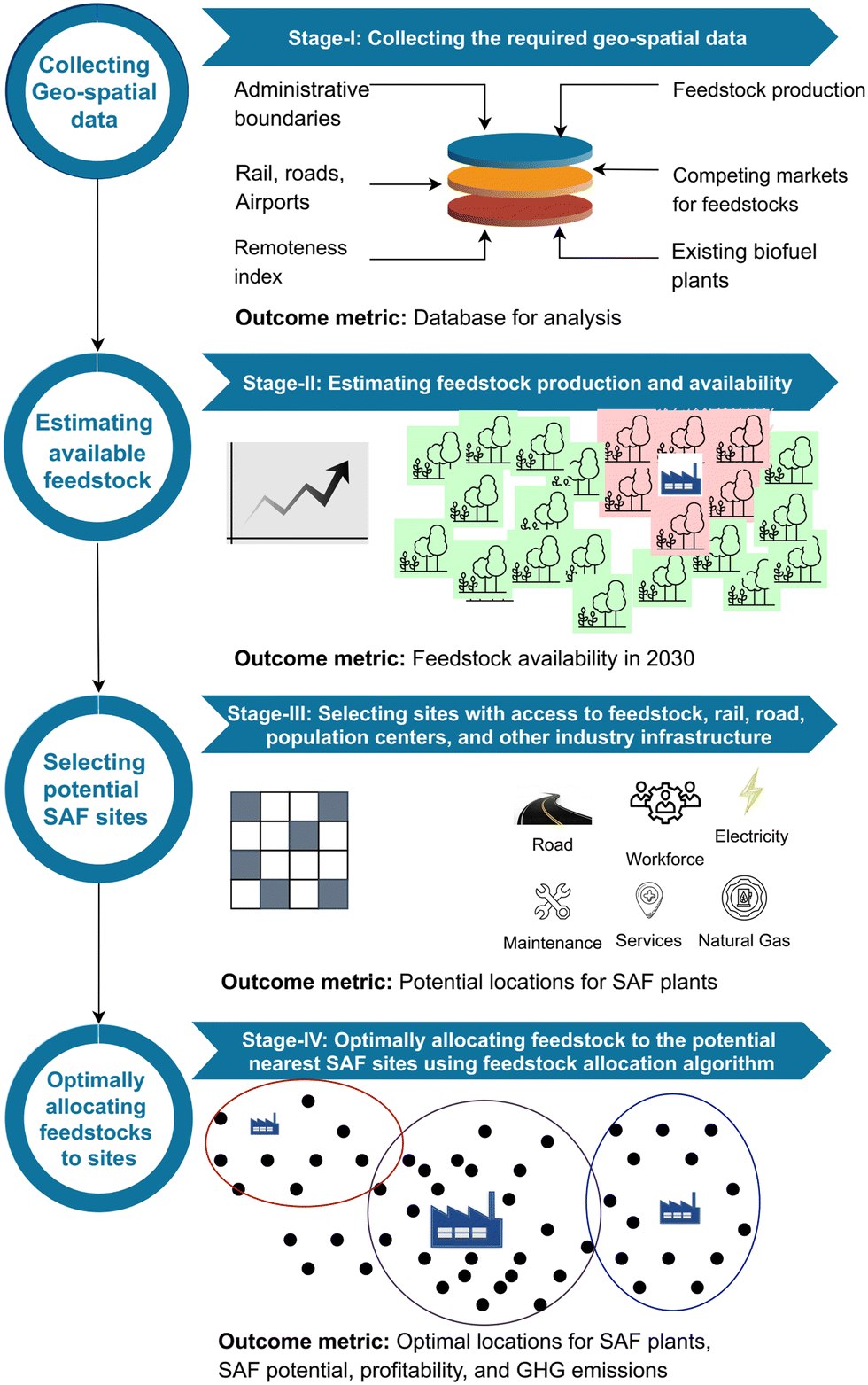

Fig. 1 Framework for estimating national SAF potential from canola by 2030. The stages I–IV indicate the steps that are sequentially followed to estimate the national SAF potential, SAF capacity and potential locations.

2.1. Geospatial data (stage I)

In stage I, the geospatial data such as feedstock production data, administrative boundaries, rail, road network, airports, existing biofuel plants, and competing feedstock markets are collected. In our case study, we collected all the geospatial data required for the study from multiple sources to create a centralized database for analysis. The Canadian administrative boundary (i.e., dissemination area, census division, province, and country) and road network (i.e., national highways and state highways) were obtained from Statistics Canada.^29,30 The rail network data were obtained from DMTI Spatial.³¹ The Canadian administrative boundaries were used to group the results for different provinces, and the road/rail network data were used to identify sites that have access to road/rail transportation. The distance calculated from the road network using geopandas was multiplied by road tortuosity to estimate the actual distance,^19,32 consistent with the literature.¹³ We have also used location data from Google maps to identify existing biodiesel plants, canola-crush plants, bioethanol plants, and airports (ESI,† Section S1). All of the geospatial data were converted to Canada Atlas Lambert projection³³ before calculating the transportation distances and proximity estimations.

2.2. Feedstock production and availability (stage II)

In stage II, the feedstock availability is estimated by first projecting the future feedstock production and subsequently removing feedstock consumed in the market. The following sections explain in detail on how the feedstock production was estimated and steps followed to eliminate the feedstock consumed in the market.

2.2.1. Feedstock production. Firstly, the production of spatially distributed feedstock is forecasted using appropriate models. In our case study, the canola production in 2030 was estimated by integrating geospatially distributed canola data and total canola production data. The geospatial canola production data were obtained from the biomass inventory mapping and analysis tool (BIMAT) business data from Agriculture and Agri-Food Canada.³⁴ The dataset consists of canola produced annually from 1986–2016 for every 10 × 10 km grid cell in Canada. Among the 17 700 data points, we have only considered grid cells with at least 10 tons per year of canola production. This curtailment has resulted in less than 0.01% “loss” of canola, and reduced the computational load by nearly 55%, i.e., to only 7600 grid cells. The total canola production dataset, i.e., 1986–2020, was sourced from the canola council of Canada.³⁵ A simple regression model was used to project how much canola would be available in 2030. Based on the regression projection, Canada can produce 24.7 MTPY of canola. The increase in production can be attributed to increases in both yield and harvested area by 2030 (ESI,† Section S2). Using 24.7 MTPY as the anticipated total canola production in 2030, the 2016 geospatial data were proportionately increased to obtain the 2030 geospatial canola production dataset for further analysis.

2.2.2. Feedstock availability. Next, the future feedstock availability is estimated by eliminating the anticipated feedstock consumption in the regional market. For our case study, we estimated the geospatial canola availability by subtracting the current (2020) canola consumption from the total canola production projected for 2030 using BIMAT GIS data. The current consumption includes canola crush plants, biodiesel facilities, and other sectors such the food industry, breweries, paints, adhesives, inks, and plastics.³⁶ The largest canola consumers are crush plants, followed by biodiesel and other sectors. The analysis focuses on existing (rather than planned) facilities due to the uncertainties surrounding planned facilities, however these are discussed further in results Section 3.3.2. A simplified material flow analysis (MFA) shown in ESI,† Section S3 gives a broader picture of the flow of canola in Canada. Since we have assumed that the consumption in current competing industries stays constant, the canola availability estimated in our study forms an upper limit. We have not incorporated any growth in other canola consuming industries due to lack of projections. Instead, our projections indicate the feedstock availability under the assumption that biojet applications are prioritized over growth in other industries. Regardless, since the direct canola consumption in other sectors are merely 3.1% (0.7 MT out of 22.1 MT in 2020, ESI,† Section S3), any additional growth in these other sectors is unlikely to significantly affect the biojet potential estimated in our study.

The canola consumption data in biodiesel industries were estimated by calculating the canola consumption from biodiesel production,³⁷ assuming an average oil content of 44%.³⁸ The data on canola consumption for the crush plants were obtained from the individual manufacturers websites^39–43 and industry reports.⁴⁴ The canola consumption data from other sectors were obtained from the canola grain elevator capacity data.⁴⁵ We assumed that these industries consumed canola from their immediate surroundings, for simplicity and due to the limited understanding of their supply chain in the public domain. After estimating the canola availability using the bottom-up approach described above, we validated with the national-level MFA numbers (ESI,† Section S3). To ensure that we did not miss any other major consumers of canola, we matched the canola availability estimated for 2030 with the actual canola exported in 2020, added to the anticipated increase in canola production by 2030. The outcome of the stage II analysis is a canola availability map that can be used to allocate canola to potential SAF sites.

2.3. Selecting potential sites for SAF production (stage III)

In stage III, the potential sites for SAF plants are selected using a series of steps. First, the sites that have access to dense feedstock producing region are selected to reduce the transportation costs. Second, among the selected sites, the remotely located sites that do not have sufficient infrastructure are eliminated. Third, among the sites that are non-remote, sites that have access to road and rail for feedstock and products transportation are selected. And lastly, among the sites that have access to rail/road, the sites that has access to population centres are selected for further optimization steps. For the case study, the following sections explains the steps followed for the canola derived SAF in Canada.

2.3.1. Feedstock accessibility. One of the first steps in screening for a potential site, is to narrow down to sites that have access to sufficient feedstock. For the case study, we selected the BIMAT sites that have access to high quantities of canola using a set of screening criteria. Since access to feedstock largely determines the plant capacity,⁴⁶ we have considered ‘canola accessibility’ as one of the site selection criteria, to eliminate sites that do not have the potential to collect sufficient feedstock within a fixed radius. Our approach differs from the literature,^12,14,16 wherein authors have considered a potential site based on the feedstock produced on/near that site, rather than the site's ability to bring in feedstock from the surrounding region to meet the plant's demand. In our work, we have deemed a site to be potentially viable only if it has the capacity to collect 214 000 tonnes of available canola from a 200 km radius (i.e., rectilinear distance). This is sufficient to meet the demand of a 100 MLPY (Million Litres Per Year) SAF plant (inclusive of all fuel co-products) – assuming a total biofuel yield of 0.467 litres per kg-canola.⁴⁷ The total fuel co-products include LPG, renewable gasoline, SAF, and renewable diesel. The main advantage of using this approach to select and to rule out sites is the substantial reduction in computational load when dealing with a high-resolution dataset (10 × 10 km grid), such as the one used in this study for Canada. The minimum 100 MLPY plant capacity was chosen based on the plant capacities of proposed renewable diesel plants in the United States.⁴⁸ Although the ultimate biofuel plant capacities range between 340 MLPY and 2780 MLPY, the minimum cut-off of 100 MLPY is a conservative and realistic choice; below this capacity, the lack of economies of scale increases the biofuel production cost. The details of how the distance between the sites was estimated and how the actual road distance was estimated from map distance are provided in ESI,† Section S4.

2.3.2. Eliminating remote locations. The next step, is to remove sites that are in extremely remote or highly populated as potential locations for SAF plants. In the case of Canada, it has the second-largest land area in the world, i.e., 9.98 million km², and therefore has many remote regions that lack basic infrastructure such as rail, road, electricity, or natural gas. In our work, we have identified these extremely remote sites using the Canadian remoteness index from Statistics Canada,⁴⁹ and eliminated them from consideration as potential biofuel sites. Briefly, the remoteness index (RI) is a numeric metric that was developed for socio-economic policy purposes to determine the proximity between service centres (e.g., hospitals, rail) and population centres (e.g., communities). It is a number between 0 and 1, wherein ‘0’ indicates a region that is non-remote (e.g., an urban municipality) and ‘1’ indicates a highly remote location. Since the remoteness index was developed with access to population centres as the basis, a lower RI value indicates a significant population and access to utilities, workforce, and community services such as hospital, fire protection, machining, and electrical services. The remoteness indices within canola-producing provinces are shown in ESI,† Section S5. In our study, we have eliminated sites for SAF production if the site's RI is above 0.4 – ‘upper threshold value’ and below 0.025 – lower threshold value. The threshold values were empirically found by locating the highest and lowest remoteness index values of sites where existing biofuel plants are situated. The rationale is that if existing biofuel plants are not located beyond the upper threshold (RI > 0.4), future plants are also unlikely to consider such sites due to remoteness and lack of infrastructure. The lower RI (RI < 0.025) regions were also eliminated because they are highly populated and, therefore, may be unsuitable due to zoning or environmental regulations. Such urban areas would also be less likely to have nearby feedstock supply, and/or face traffic restrictions and other challenges for feedstock delivery.

2.3.3. Access to rail and road. Proximity to highway, rail, and natural gas are always met for operational reasons in North American oil-seed crushing facilities.⁵⁰ Therefore in the next step, the sites that have access to connectivity must selected and the rest are eliminated. For our case study, we selected sites that have access to both rail and inter-provincial and state highways for feedstock and product transport. Road and rail connectivity is vital for transporting canola from the farm to the processing facility and transporting fuel products from the SAF plant to the market. According to the Canola Council of Canada, about 40% of canola is delivered to processing facilities directly from the farm using a truck.⁵¹ In Canada, the existing biofuel plants are, on average, 4 km from major highways and within 1.2 km of major railway lines (ESI,† Section S6). Our study has considered a site as a potential SAF site only if it is located within 1 km of existing rail lines and roadways, based on our communication with industry experts and project developers.²⁷ Note that some studies have considered a distance of up to 5 km for rail,¹⁸ in which case the additional cost of constructing a connecting rail spur and land procurement costs should be accounted for in the supply chain cost model.¹³

2.3.4. Access to population centres. Lastly, the sites are narrowed to a final set of candidates using population centres as a proxy for various required supporting infrastructure. Biofuel industry site selection factors typically include locations with access to water, access to labour and proximity to co-product markets (ESI,† Section S7). These factors are often implicitly incorporated by choosing sites that are closer to cities/towns, as proxies,^{11,17,18,23–25} and so we adopt this as a site selection criterion. Unlike the previous step involving the remoteness index wherein the unwanted sites are removed, the goal of this step is to select a limited number of sites that show the strongest potential for SAF plants.

For the case study in Canada, the GIS location and population data of cities/towns were obtained from the simplemaps database,⁵² and we have considered only cities/towns with a minimum population of 1000.³² Some studies have considered sites with a larger population range, between 3000–10 000²³ or, in some cases, only large cities.^11,18 In Canada, all existing bioethanol and biodiesel plants are located within 12 km of towns/cities (ESI,† Section S6). However, for this study, we have considered a site to be eligible if it is located within a 20 km distance from existing towns/cities based on a Biofuels Canada industrial feasibility study report.²² The greater distance (20 km instead of 12 km) reflects practical access to labor and supporting infrastructure, while also recognizing that as more biofuels plants are built, they may need to be further away from existing urban centers to avoid overlapping demand for nearby feedstock.

Overall, in stage III, the potential sites for constructing a SAF plant were identified based on industry site selection criteria. A map containing all potential BIMAT sites was then used in the next stage to identify the optimal locations for the plant and, subsequently, SAF potential.

2.4. Optimal feedstock allocation model (stage IV)

Having narrowed down the feasible sites, the final step is to select optimal sites from among these candidate sites. Thus, the first part of stage IV requires the development of modules to calculate the relevant characteristics of potential plants for each site. This may include coordinated efforts to maximize feedstock utilization, individual corporate efforts to maximize profits, policy targets related to minimizing environmental impact or maximizing gains to local communities and so on. In this study, we focus primarily on efficiency (maximizing feedstock utilization) and financial gains (maximizing profits), while analyzing the resulting greenhouse gas emissions (GHG). Thus, the first step is to develop additional modules to assess the economics of plant operations through techno-economic analysis (TEA) model, and to estimate GHG emissions through life cycle assessment (LCA) models. Subsequently, the national SAF capacity and potential locations for SAF plants are estimated using two optimal plant allocation approaches: maximum feedstock utilization and maximum profitability. The following subsections explain how the modules were developed for the case study on canola SAF and the model parameters used in the allocation approaches.

2.4.1. Modules to calculate site characteristics.
2.4.1.1. Financial module. A financial model is required to estimate the profitability of a SAF plant at each identified potential location for optimization. Depending on the scenario, the TEA model can consider a standalone facility or an integrated facility that processes canola and produces SAF in the same site. In our case, a modified TEA model was developed based on our previous work on a HEFA-based SAF plant in an integrated crushing and processing facility.^47,53 The CAPEX and OPEX were estimated using the mass and energy balances derived from ASPEN modelling and verified with industry sources.²⁷ Several TEA parameters and data sources were used in the financial model to reflect the canola SAF operations specific to Canada and they are documented in ESI,† Section S8. The model includes historical prices for feedstock, energy inputs, and co-products. We do not project future changes in canola price (which themselves may experience upward pressure due to a growing SAF market), but include a canola price sensitivity scenario in ESI,† Section S15. We further include an incentive of $0.6 CAD per L to ensure that SAF plants can be profitable (IRR > 15% for our resulting locations). Although larger than any current Canadian incentive, this is in line with the upper end of the range offered by the US Inflation Reduction Act ($1.25–1.75 USD per gallon).⁵⁴ The implicit assumption is that the domestic SAF market will require sufficient support to compete with US buyers/producers and so this study assumes generous incentives will be in place before questions of total domestic potential become relevant.

Finally, the transportation cost in the financial model is estimated from feedstock transport cost, and product transport cost. For our case study, the canola transportation cost was adapted from the canola truck cost reported by the Canola Council of Canada. Since almost 40% of the canola is transported to the processing facilities using trucks,⁵¹ for simplicity, we have considered canola to be transported via truck to the production facility. We did not analyse the impact of longer shipment of canola via long distance rail. For the refined products, we have considered truck transportation to nearby markets and airports. The trucking costs were adapted from American Transportation Research Institute (ATRI).⁵⁵ A tanker truck capacity of about 45 000 litres is assumed, and a transport cost of 1.542 CAD per km for the specialized sector is used in our study.⁵⁶ We have assumed trucking for transporting, instead of pipeline and rail cars, for a few reasons. In the case of pipelines, there is a lack of existing infrastructure, and the possibility of transporting SAF to the refinery (for blending) and subsequently to airports in the canola-producing region seems unrealistic because the pipeline network and flow direction are aligned with British Columbia. And in the case of rail, local scenarios in the prairies dictate many constraints, such as limited availability of railcars and the non-alignment of rail network with locations where SAF is produced versus where it would be blended or used. As such, since the infrastructure required to transport the SAF products is not within scope and therefore we assume truck transport for simplicity.

2.4.1.2. LCA module. An LCA module is required to estimate the average carbon intensity of the selected plant locations and to understand the implications of regional variations in carbon intensity of SAF. Since GHG mitigation is a core motivation behind SAF development, we coupled our potential/logistics model with an LCA model that enables us to estimate GHG intensity in selected optimal sites. We assess these environmental impacts by adapting life cycle greenhouse gas (LC-GHG) results from our prior study. The LC-GHG at potential sites depends on local characteristics such as soil, previous use of the land before canola, regional fertilizer consumption, and local farming practices. Obnamia et al.,⁵⁷ reported the LC-GHG emissions of canola-derived SAF for each Canadian reconciliation unit (RU). An RU is a regional zone in Canada for reporting data land and activity from multiple agencies; an RU is considerably larger than the BIMAT sites used for analysis in our study. The LC-GHG emissions of the individual reconciliation units with and without land use (LU) and land management changes (LMC) are given in ESI,† Section S9. For the purpose of the present paper, we assume (1) that each RU is uniform in its emissions even though the boundaries are arbitrary for administrative reasons and (2) that, for carbon accounting, the average historical LU and LMC still apply to future uses.

Once optimal sites are selected (Section 2.4.2), we correlated the available canola in the RU to the LC-GHG emissions from these reconciliation units and estimated weighted average LC-GHG emissions of the optimal locations, which draw canola from multiple RUs having different LC-GHG emissions.

2.4.2. Optimal site selection. In the optimal site selection, optimization algorithms are developed to optimally allocate the feedstock to final sites for SAF production. In our case study, we demonstrate two heuristic optimization procedures to select from among the final candidate sites. (1) A maximum feedstock utilization algorithm is used to identify potential locations for SAF plants by maximizing the amount of canola captured. The goal of this approach is to get an upper bound of the SAF potential by allocating canola to the nearest plant. (2) A maximum profitability algorithm is used to identify potential locations by maximizing the profitability of the SAF plant locations. The goal of this approach is to minimize the cost of purchasing and transporting canola, the cost of processing, and the cost of delivery to airports.
2.4.2.1. Maximum feedstock utilization approach. In the maximum feedstock utilization scenario, the goal was to determine Canada's maximum canola SAF potential when all of the available canola is accessible to the SAF production sites. However, while allocating, we assumed that only a fraction of the canola theoretically available is actually available for a prospective SAF plant. In industrial feasibility studies, this guideline is typically followed to lessen any unanticipated supply chain risk due to weather events and market competition that would result in feedstock basis price escalation and poorer financial profitability of a biofuels plant.²⁷ Depending on the region (rural vs. urban), extent of local consumption of canola, and export market strength, the guideline on potential supply can vary between 25–50%. Although 100% utilization is theoretically possible, investors and plant producers are generally uncomfortable assuming greater than 50% of the available feedstock is available to new industry users.²² Therefore, in our model, we have considered scenarios wherein a new biofuels plant can capture only 25, 35, and 45% of the maximum available feedstock available in a region. The percentage of available canola is a critical constraint because it can significantly influence how many biofuel plants (and other competing users) can co-exist in a canola producing region, which in turn limits national SAF plant capacities and potential SAF production. Policy makers need to be aware of these constraints and the range of outcomes that may arise.

The national canola SAF potential in the maximum feedstock utilization approach was estimated based on the following steps:

(i) The canola produced in each BIMAT site (10 × 10 km canola producing region) is allotted to the nearest potential SAF plant site. The step is consistent with how the industry operates to reduce transportation costs.⁵⁸

(ii) After allocating all of the canola to the nearest potential SAF site(s), the canola allocated to each SAF site is summed to verify if there is sufficient canola to meet supply needs for a (minimum) 100 MLPY plant.

(iii) If the SAF site has sufficient canola to run a minimum 100 MLPY plant, then the SAF site is regarded as a potential site for SAF plant construction, and therefore retained as a candidate.

(iv) After allocation, if any of the SAF sites have insufficient canola to run a minimum 100 MLPY plant, then the site with the lowest amount of canola is eliminated, and the canola is re-allocated to nearby potential sites. Step (iv) is repeated until all remaining sites surpass the 100 MLPY threshold.

(v) The above step is repeated until all the insufficient canola sites (<100 MLPY) are eliminated, and the sites with sufficient feedstock to run a minimum of 100 MLPY SAF plant are retained.

The outcome of the maximum feedstock utilization scenario is a set of optimal locations that can serve as locations for canola SAF plants, with the goal of maximizing the national SAF potential from canola.

2.4.2.2. Maximum profitability approach. In practice, biofuel investors are most likely to choose locations that are expected to be highly profitable. Therefore, the goal in this approach was to find the most profitable locations for the SAF plants and find the individual plant capacities for estimating the national SAF potential from canola. Similar to the previous scenario, only a fraction of canola (25%, 35%, and 45%) is assumed available for a prospective SAF plant based on the guideline followed by financial institutions and investors in feasibility studies. The following steps were followed to estimate the national SAF potential from canola, most profitable locations for SAF plants, and internal rate of return (IRR) of canola SAF plants using the HEFA technology.

(i) The amount of canola within the 200 km collection radius of every potential SAF site was estimated and allocated to the potential site.

(ii) For each potential SAF site, the canola collection cost, processing costs, product transportation costs, and IRR were estimated.

(iii) The site with the highest IRR was selected as the most profitable location, and the canola available within a 200 km radius was removed from the feedstock map, and the existing feedstock allocation was dissolved. This is similar to the situation in practice a biofuel plant is set up in a particular location. The amount of feedstock to run that plant is then unavailable in that region, limiting or precluding construction of another plant.

(iv) The above steps were repeated sequentially until the selected profitable sites no longer had enough feedstock for a 100 MLPY SAF plant.

We have used IRR as a profitability measure in our financial model^59,60 and assumed 200 km as the maximum canola collection distance, based on historical practises for biofuels plants. Beyond this distance, transportation costs may increase dramatically, because of practical limits on trucking feedstock from canola production locations and storage depots.

3. Results

3.1. Canola production and availability (stage II)

In stage II, the canola production in Canada for 2030 and its potential availability after domestic consumption were estimated. Fig. 2 shows the projected canola production data for 2030 in Canada. The light yellow grids indicate low canola producing regions, with about 10–1000 tonnes per year, and the dark red grids indicate a high canola producing region, with more than 12 000 tonnes per year. Among the three provinces, in 2030, nearly 80% of the canola is expected to be produced in Alberta and Saskatchewan, and about 20% in Manitoba, which agrees with the current distribution.⁶¹ The projected canola production in 2030 is 24.7 million tonnes (MT), 32% higher than in 2020. The increase in production can be attributed to the anticipated 15% increase in yield and a 32% increase in harvested area by 2030 (ESI,† Section S2). Although our projection suggested a moderate 24.7 MT canola production by 2030, the Canola Council of Canada⁶² is expecting production of 26 MT as early as 2025. However, despite that, we have retained our projection of 24.7 MT in our model as a conservative estimate, considering uncertainty in weather events and crop planting decisions by farmers.

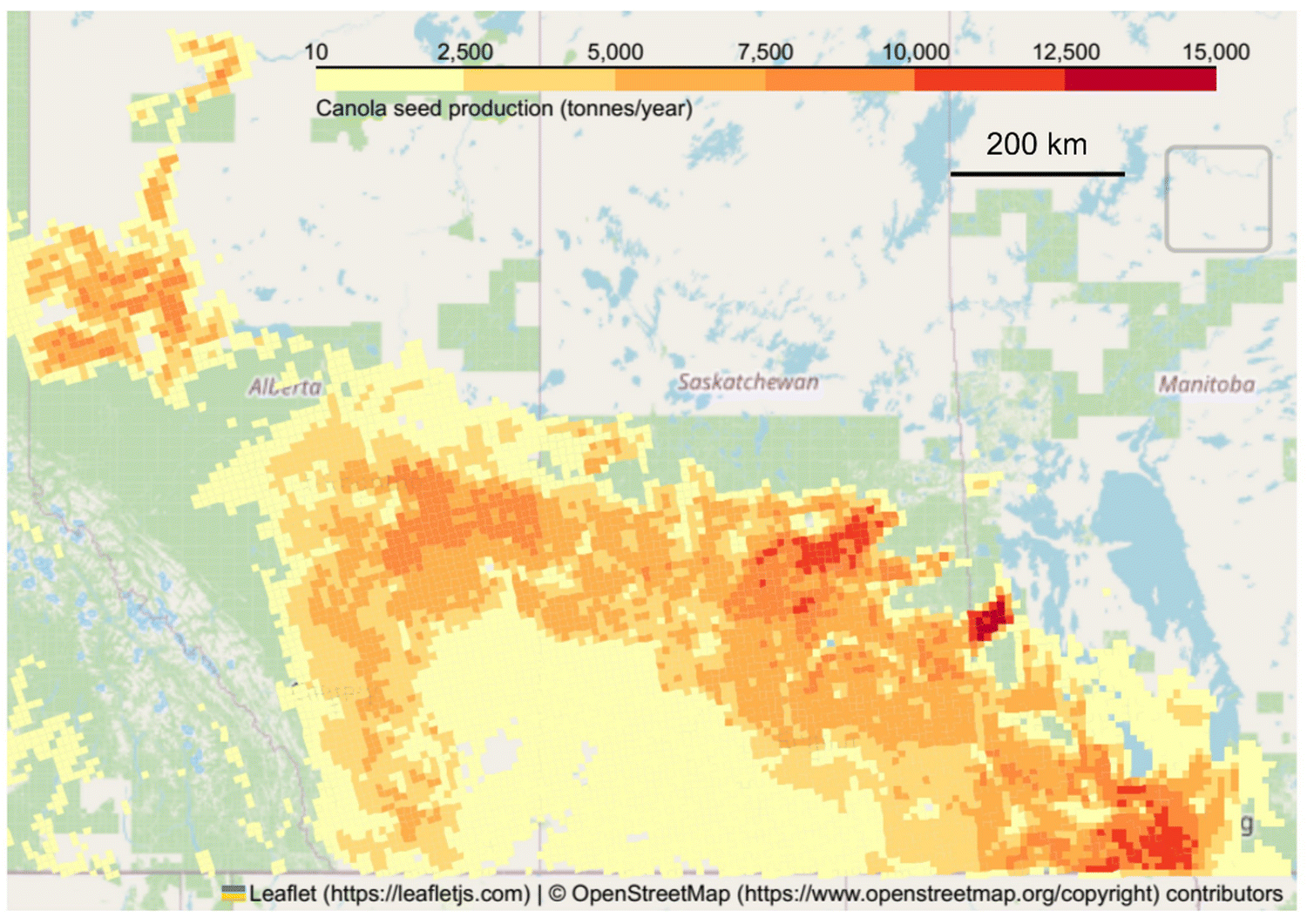Fig. 2 Projected canola production (tonnes per year) in 2030 across the provinces of Alberta, Saskatchewan, and Manitoba. Each data point corresponds to a 10-by-10 km site obtained from the BIMAT database.

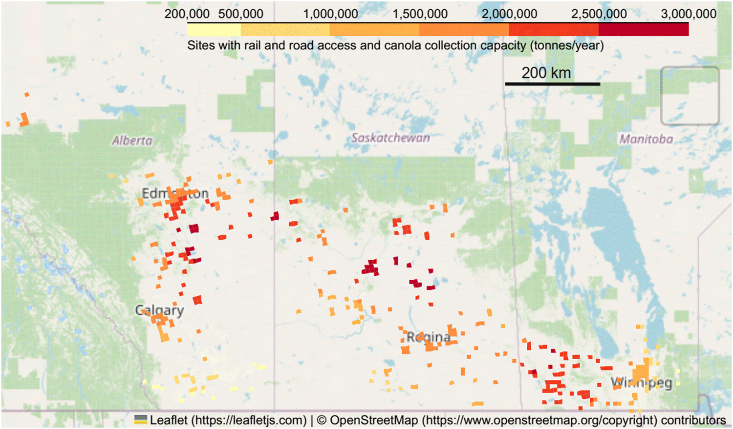
Fig. 3 shows the canola available in 2030 after accounting for domestic canola consumption. The location-tag symbols on the map indicate canola crush plants and biodiesel plants that consume canola as feedstock. The empty round spaces in the choropleth map indicate zero canola availability because of assumed consumption from the industries. Out of the 24.7 MT anticipated canola production in 2030, the crush plants (and integrated biodiesel plants) are expected to consume 8.8 MT, biodiesel (only) plants 0.04 MT, and other sectors around 0.73 MT. The 15.2 MT of leftover canola is expected to be available for exports or other domestic uses. In our study, we have assumed that the leftover canola can be used to produce SAF.⁴⁶ This assumption is consistent with the Canadian Sustainable Aviation Fuel (C-SAF) industry association's view that the exported canola can be deployed locally with sufficient incentives and appropriate policies.⁶³

Fig. 3 Canola availability in Canada in 2030 after domestic consumption from local industries. The small red and yellow squares indicate canola production, the location tags with pins indicate canola crush plants and the local tags with industry symbol represents canola-biodiesel plants.

3.2. Selecting potential sites for SAF production (stage III)

The results below are based on the steps followed sequentially to select the potential sites for SAF plants, as described in the stage III methodology.

3.2.1. Selecting sites with access to canola and eliminating remote sites. Proximity to feedstock is one of the key site selection criteria for potential sites for a biofuel plant.^22,58 Therefore, in our study, we selected potential sites for SAF plant only if they have access to sufficient canola to run a 100 ML per year SAF plant. Considering a total product yield of 467 litres per tonne of canola,⁵³ this translates to 214 130 tonnes of canola. Fig. 4 shows the BIMAT grid/sites with a canola collection capacity of more than 214 000 tonnes (i.e., 100 ML per year SAF). The dark red sites in the middle of the canola producing region indicate locations with access to large amounts of canola, and the light yellow sites near the edges of the map indicate regions with access to relatively low amounts of canola. We found that after including the canola accessibility criteria, about 6800 canola producing sites (i.e., grid cells) are suitable to supply a SAF plant in Alberta, Saskatchewan, and Manitoba.

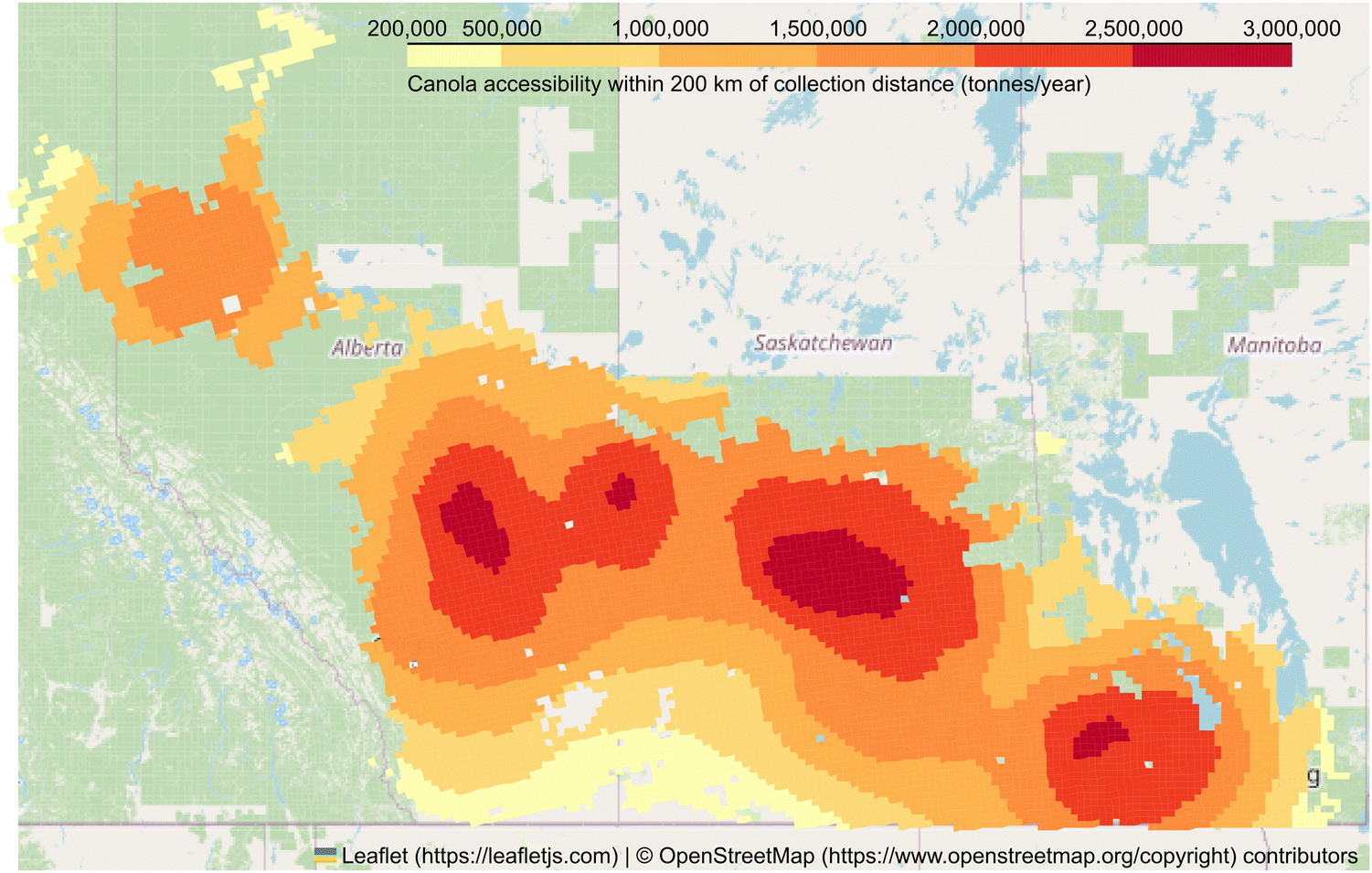Fig. 4 Canola collection capacity (tonnes per year) of every BIMAT site by 2030. Each BIMAT site is a 10-by-10 km canola producing region, and there are about 6800 sites on the map.

Among the 6800 canola production sites where a biofuels plant could be located (Fig. 4), some are situated in remote regions that lack access to basic industrial infrastructure. We eliminated these remote sites if the Canadian remoteness index (RI) is less than 0.025 or greater than 0.4. After removing the remote locations, the number of potential SAF sites was reduced by about 30% from 6800 to 4800. As shown in Fig. 5, the unplotted regions in the contour regions represent the eliminated sites. The sites removed include those that are highly populated (RI < 0.25) where industries are unlikely to be constructed and sites that are extremely remote (RI > 0.4), where lack of access to infrastructure makes it difficult/unlikely to set up a biofuel plant. Most of these remote regions were located in the southern region connecting southeast Alberta to southwest Saskatchewan, and in northern Saskatchewan and Manitoba. These regions are among the most remote regions (RI > 0.5) with a significantly lower population, as shown in the remoteness index map (ESI,† Section S5).

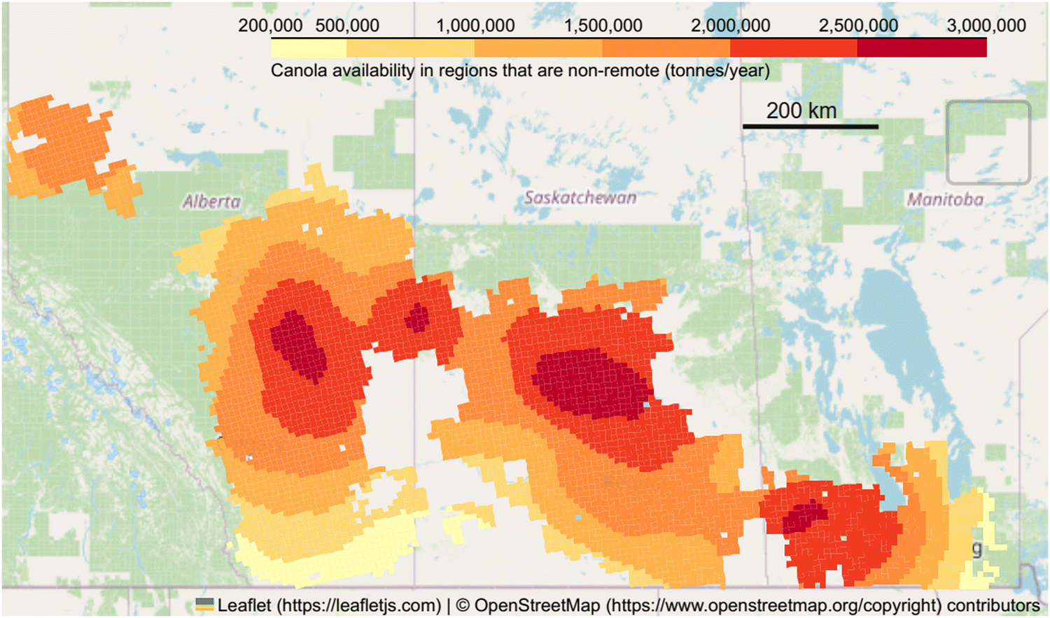Fig. 5 Canola producing BIMAT sites (10-by-10 km) that are not located in remote locations as estimated using the Canadian remoteness index.

3.2.2. Access to rail and road connectivity. Access to rail and road are essential for transporting canola from the agricultural field to the SAF facility and transporting products to market. It is one of the key reasons all canola crush plants and biodiesel plants are located next to a major rail or road network in Canada (ESI,† Section S10). Fig. 6 shows the BIMAT sites with access to rail and road connectivity. The potential SAF sites have significantly reduced from about 1400 to 370 – an almost 92% decrease suggesting that only a few potential sites have access to rail and road infrastructure and are suitable for biofuel plants. Most potential sites are concentrated around major and smaller cities such as Calgary, Red Deer, and Edmonton in Alberta, Saskatoon, Regina and Yorkton in Saskatchewan, and near Winnipeg in Manitoba. The areas around Camrose, Alberta and Lloydminster, which borders Alberta and Saskatchewan, also have suitable sites.

Fig. 6 Potential canola producing sites in Canada that have access to both rail and road connectivity.

3.2.3. Access to population centres. Access to population centres is also considered an essential site selection criterion, to provide access to labour and community services such as welding, electrical shop, plumbing, schools, fire protection, and hospitals.²² Fig. 7 shows the potential SAF sites within 20 km of population centres such as towns/cities and that have access to rail/road. After including the criterion for proximity to population, potential SAF sites were reduced from about 370 to 320 – a 14% decrease. The minor reduction in the number of sites is because most sites with access to both rail and road were already located close to towns/cities. It could be one of the reasons some studies have even directly selected cities/towns as the potential sites without explicitly considering rail, road, and access to services in the site selection analysis.^11,18,23 Although this approach might reduce the complexity of the analysis, it may not be optimal when the feedstocks are concentrated in rural areas away from population centres.

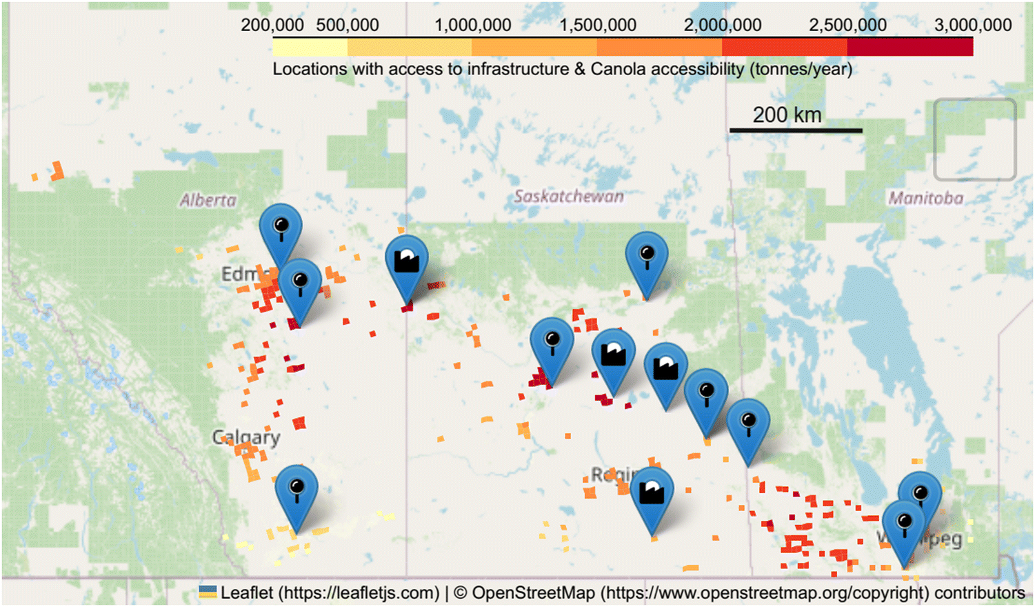Fig. 7 Potential canola SAF production sites having access to rail, road, and population centres. The small red and yellow squares indicate canola production, the location tags with pins indicate canola crush plants and the local tags with industry symbol represents canola-biodiesel plants that use canola as a feedstock.

3.3. Optimal feedstock allocation model (stage IV)

The national canola SAF potential and optimal locations were estimated by allocating the available canola to the potential sites under two scenarios: maximum feedstock utilization and maximum profitability.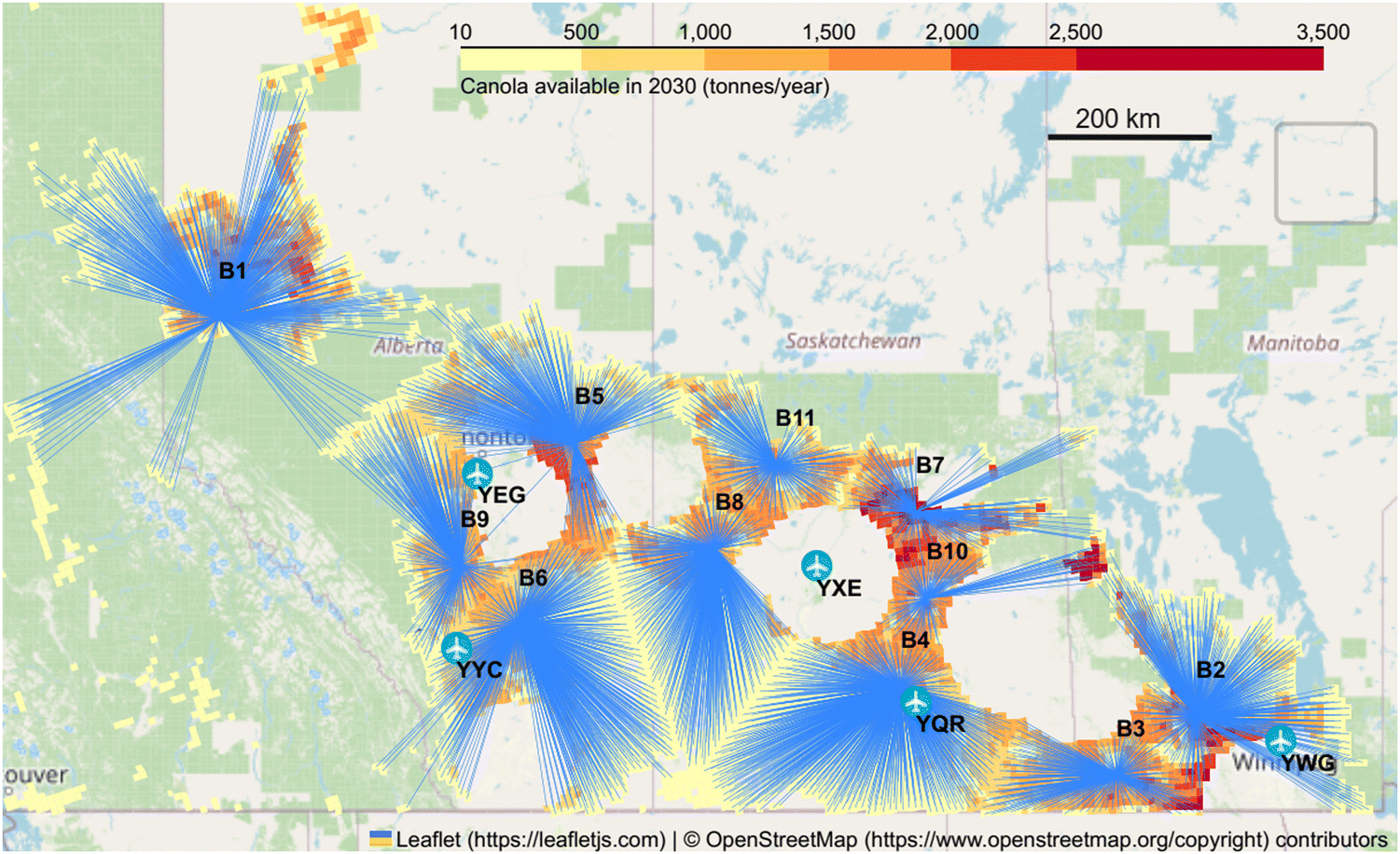

3.3.1. Maximum feedstock utilization scenario: National canola SAF potential. In the maximum feedstock utilization scenario, we identified potential locations and estimated the maximum SAF potential using the heuristic optimization methods described in the methods section. Fig. 8 shows a map in which all the available canola is optimally allocated to potential sites and Table 1 shows the optimal locations B1 to B11 and their SAF potential for 45% and 25% feedstock accessibility criteria. For a 25% guideline on feedstock accessibility, annually about 1 billion litres (BL) of SAF can be produced from the canola producing regions and for a 45% feedstock accessibility guideline, about 1.8 billion litres of SAF can be produced. Specifically, with supply restricted to 25% of available canola, Alberta can supply about 390 MLPY (Million Litres Per Year), Saskatchewan about 400 MLPY, and Manitoba about 210 MLPY SAF by 2030.

Fig. 8 Canola allocated to SAF sites in the optimal feedstock utilization scenario for a 25% feedstock accessibility criteria. B1–B11 are the optimal locations for canola SAF plants. The major airports are indicated by a small airplane symbol inside a circle and the letters near the airports indicate the IATA codes: YEG-Edmonton, YYC-Calgary, YXE-Saskatoon, YQR-Regina, and YWG-Winnipeg.

Table 1 SAF potential at sites identified in the maximum feedstock utilization scenario at 25% feedstock accessibility criteria. The fuel co-products include LPG, renewable gasoline, naphtha, and renewable diesel

Plant	Canola capacity (tonnes per year)	SAF (MLPY)	Fuel co-product (MLPY)
B1	462 750	125	217
B2	418 867	113	196
B3	381 960	103	179
B4	373 409	101	176
B5	365 664	99	172
B6	364 736	98	170
B7	325 408	88	153
B8	312 560	84	146
B9	274 053	74	129
B10	254 630	69	120
B11	226 785	61	106
Total	3 760 820	1015	1764

---

The SAF produced in these 11 locations could be used to supply SAF to major airports in the three provinces. Table 2 shows the SAF demand in international airports located in the canola producing provinces Alberta, Saskatchewan, and Manitoba. A total production of 1000 ML, at a 25% feedstock accessibility guideline, should be able to meet the HEFA based annual SAF demand in Calgary (323 ML), Edmonton (150 ML), Regina (28 ML), Saskatoon (36 ML), and Winnipeg (90 ML), based on the ASTM SAF blending limit of 50% for HEFA-derived fuels. The excess SAF, if any, may be sent to Vancouver to meet the SAF demand in Vancouver, the second largest airport in Canada.

Table 2 Potential SAF demand in selected international airports in the canola producing region in Canada. The demand was estimated considering 50% blending for HEFA based SAF.⁶⁴ Due to lack of recent data, the jet fuel consumption in 2019 were projected using the increase in passenger traffic observed in the airports with details provided in ESI, Section S14

Airport city	Province	Possible SAF demand in 2019 (in million litres)	Jet fuel consumption and year (in million litres)
			Available data	Projected for 2019
a Indicates lack of publicly available data and therefore, projected based on passenger traffic from a similar sized Winnipeg airport.
Calgary (YYC)	Alberta	323	518 ML, 2013^65	646 ML
Edmonton (YEG)	Alberta	150	235 ML, 2011^66	301 ML
Saskatoon (YXE)	Saskatchewan	36	68 ML, 2015^a	71 ML
Regina (YQR)	Saskatchewan	28	59 ML, 2015^a	56 ML
Winnipeg (YWG)	Manitoba	90	181 ML, 2019^67	181 ML
Vancouver (YVR)	British Columbia	1088	1400 ML, 2011^68	2177 ML
Total		1715

---

We also estimated the total SAF production potential from canola in Canada by 2030 under different feedstock accessibility scenarios. Table 3 shows the national canola SAF potential for Canada and the SAF potential in Alberta, Saskatchewan, and Manitoba, considering various feedstock supply guidelines applied by industries and investors in their feasibility studies. As expected, an increase in the feedstock accessibility criteria proportionately increased the national SAF potential, i.e., an 80% increase in the fraction of feedstock accessible from 0.25 to 0.45 increased the national SAF potential from canola by 80% from 1 billion litres to 1.8 billion litres. Among the provinces, Saskatchewan and Alberta have the greatest potential for SAF, sharing almost similar capacity, i.e., 722 ML and 779 ML. Manitoba, on the other hand, has less than half of the SAF potential of Alberta due to lower availability of canola. Similarly, with an increase in the fraction of accessible feedstock from 0.25 to 0.45, the amount of canola available increases nearly 80% from 3.76 MT to 6.78 MT. Note that for reference, the total canola available is 15.2 MT, without any restrictions on feedstock availability.

Table 3 Comparison of national SAF potential and canola that can be captured under the maximum feedstock utilization scenario for various industry guidelines for feedstock accessibility

Feedstock accessibility guideline (% of total)		25%	35%	45%
SAF	Alberta	396 ML	554 ML	722 ML
	Saskatchewan	403 ML	613 ML	779 ML
	Manitoba	216 ML	253 ML	329 ML
	Total	1015 ML	1420 ML	1830 ML
Canola	Alberta	1.46 MT	2.1 MT	2.67 MT
	Saskatchewan	1.49 MT	2.3 MT	2.88 MT
	Manitoba	0.8 MT	0.94 MT	1.22 MT
	Total	3.76 MT	5.3 MT	6.78 MT

---

3.3.2. Best profitability scenario: optimal SAF locations and profitability. In the best profitability scenario, the optimal locations and SAF potential were estimated based on the profitability of a biofuels plant at each site. We have selected locations one by one, mimicking the scenario wherein industries construct SAF plants, starting from the most profitable options.

Fig. 9 shows the canola allocated to the most profitable SAF sites for 25% feedstock accessibility criteria (RT) and 200 km canola collection distance. As shown in Table 4, seven SAF plants are feasible when plants are constructed one-by-one based on profitability with at least three sites in Alberta, three in Saskatchewan, and one in Manitoba. Some key locations for SAF/renewable-diesel facilities are Camrose, Grande Prairie, and Calgary in Alberta, Saskatoon, Weyburn, and North Battleford in Saskatchewan, and Portage-la-Prairie/Brandon in Manitoba. The chosen seven optimal locations are located close to one of the five international airports such as Edmonton, Calgary, Saskatoon, Regina, and Winnipeg. At the time of writing this article, two canola biofuel plants were planned in Canada, and they are located close to these seven sites identified in our study. The first plant is in Edmonton at Imperial Oil's Strathcona refinery,⁶⁹ which is 70 km from Camrose and the second plant is in the Regina refinery site from Federated Co-operative Limited,⁷⁰ which is 100 km from Weyburn. These locations are based upon co-location at existing industrial complexes rather than green-field sites. Note that Edmonton and Regina were among the best 320 locations identified during site selection in Section 3.2.3. We did not include any upcoming plants for estimating canola availability because of uncertainties around the exact amount of canola used and the date of entry in service, however these are included in ESI,† Section S13 for reference.

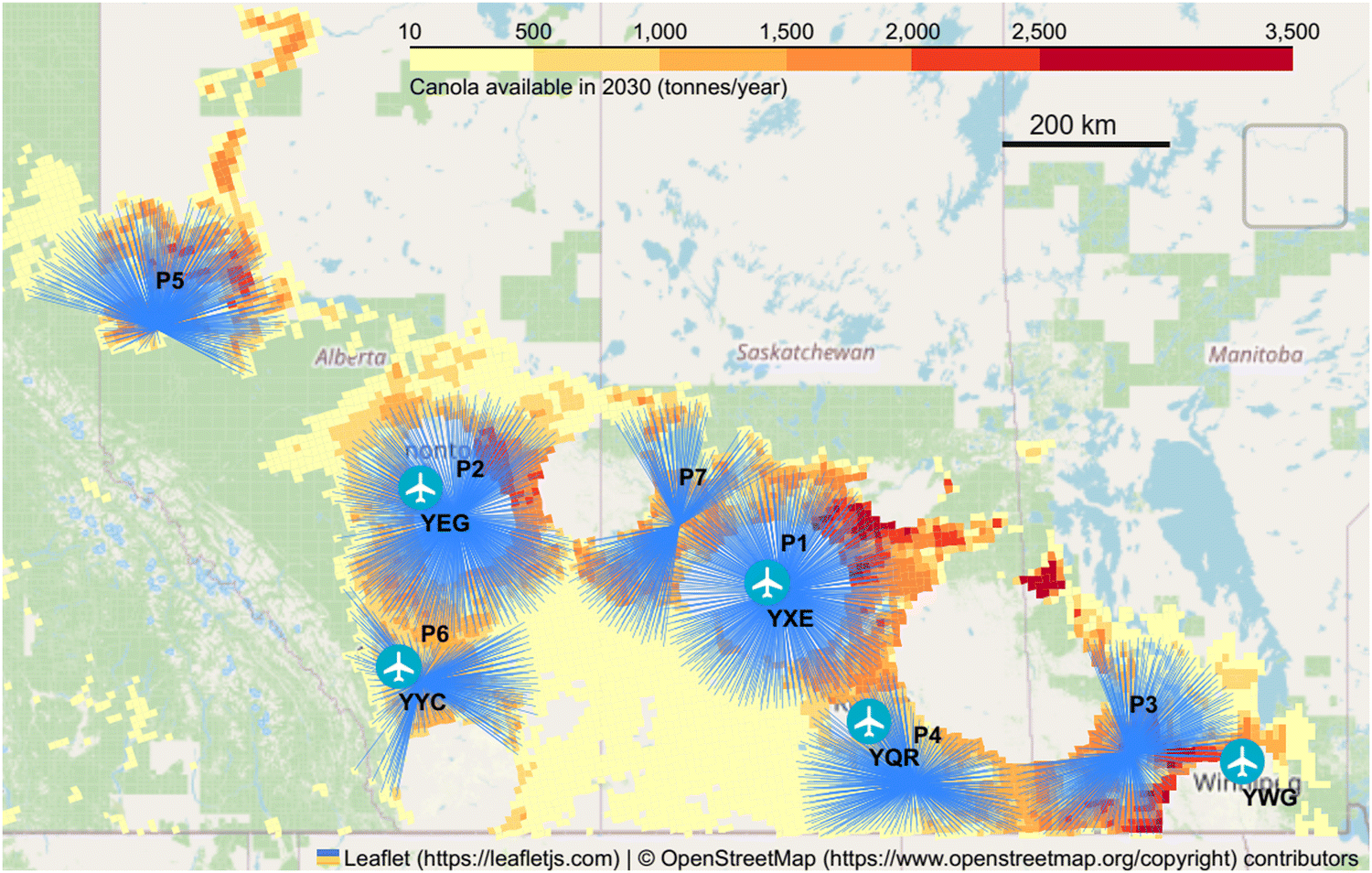Fig. 9 Canola allocated to optimal locations identified in the best profitability scenario for a 200 km feedstock collection distance and 25% feedstock accessibility criteria. P1–P7 are the potential SAF plants with P1 being the most profitable and P7 the least, and the letters indicate IATA codes: YEG-Edmonton, YYC-Calgary, YXE-Saskatoon, YQR-Regina, and YWG-Winnipeg.

Table 4 SAF potential at sites identified in the maximum profitability scenario for 25% feedstock accessibility criteria

	Nearest city	Nearest airport	Canola capacity (tonnes per year)	SAF (ML)
P1	Saskatoon	YXE	706 000	191
P2	Camrose	YEG	643 000	174
P3	Portage-la-Prairie	YWG	610 000	165
P4	Weyburn	YQR	315 000	85
P5	Calgary	YYC	402 000	109
P6	Grande Prairie/Brandon	YEG	215 000	58
P7	North Battleford	YXE	254 000	69
Total			3 145 000	851

---

Table 5 shows the IRR of these optimal plant locations (P1–P7) and associated sensitivities to the feedstock accessibility guideline, arranged in the order of profitability. It is clear from the table that the IRR increase with the plant's capacity, suggesting that the economics of scale play a role in the overall profitability. The profitability of the seven plants varies between 15 and 22%, with the most profitable locations being close to Saskatoon, Saskatchewan and Camrose, Alberta because of the greater availability of canola. The lowest profitability locations were close to North Battleford and Melfort in Saskatchewan because of the lower canola availability. Depending on the 25–45% feedstock accessibility guideline used, the profitability (IRR) of the largest plant (>500k tonnes) ranges between 22–28%, and the IRR for the smallest plant ranges between 16–19%, as shown in Table 5. The IRR results in the table are derived from average canola prices over 2016–2021, incorporating an assumed incentive of 0.6 $ per L. As outlined in ESI,† Section S15, achieving comparable IRR outcomes with elevated feedstock prices necessitates an increase in the incentive up to 1.5 $ per L, reflecting the peak prices observed in 2022.

Table 5 Optimal SAF plant locations and their profitability (IRR) for 25% feedstock accessibility criteria for a 0.6 $ per L incentive. Airport IATA codes: YEG-Edmonton, YYC-Calgary, YXE-Saskatoon, YQR-Regina, and YWG-Winnipeg

Optimal location	IRR (%) and capacity for various industry feedstock percent accessibility criteria
	IRR at 25% feedstock accessibility	Capacity (tonnes)	IRR at 35% feedstock accessibility	Capacity (tonnes)	IRR at 45% feedstock accessibility	Capacity (tonnes)
P1	24	706 000	27	988 000	28	1 271 000
P2	23	643 000	26	901 000	28	1 158 000
P3	23	610 000	25	854 000	27	1 098 000
P4	19	315 000	21	440 000	23	566 000
P5	18	402 000	21	563 000	22	724 000
P6	17	215 000	19	356 000	21	457 000
P7	17	254 000	19	301 000	21	387 000
P8	—	—	16	221 000	18	285 000
	20 (avg)	3.15 MT	22 (avg)	4.6 MT	23 (avg)	5.9 MT

---

Table 6 shows the total SAF produced, percentage of canola captured, and the average IRR of plants in the best profitability scenario. The total SAF produced from canola under the 25% feedstock supply guideline is 850 ML, with a corresponding canola consumption of 3.13 MT. For the same 25% feedstock accessibility guideline under the maximum feedstock utilization scenario, the maximum SAF produced is 1015 ML, over 20% larger than in the maximum profitability scenario. This shows a potentially important role for coordinated site selection to ensure Canada can realize its maximum production potential. Otherwise, sequential decisions based on maximum profitability are likely to leave out a certain percentage of the feedstock, stranding some canola in regions with insufficient density to justify construction of another plant.

Table 6 Summary of optimal SAF plant locations, IRR, and canola consumed in the best profitability scenario for various values of the feedstock accessibility guideline

Feedstock accessibility guideline	25%	35%	45%
Canola consumed	3.15 MT	4.63 MT	5.95 MT
% Canola captured among available canola	83%	88%	88%
Canada SAF	850 ML	1250 ML	1600 ML
No. of plants	7	8	8
Avg. IRR of plants	20%	22%	23%

---

At the upper limit of the feedstock accessibility guideline, the national SAF potential from canola increases because the amount of canola available increases. Moving from the lower limit of the feedstock accessibility guideline (25%) to the upper limit (45%), the amount of potential SAF increases from 850 ML to 1600 ML. Similarly, with the increase in available feedstock, the SAF plant profitability also increases, by 16%, due to the increase in the average size of the SAF plant in the canola producing region.

3.4. Canola availability and regional life cycle GHG emissions

In addition to estimating the canola availability and optimal locations for SAF plants, we also estimated the life cycle GHG emissions (LC-GHG) to highlight the range of GHG emissions (g CO₂eq per MJ) values that can be anticipated in these optimal locations. These regional LC-GHG emissions results could be helpful for fuel producers when deciding on a particular location for the SAF plant, and relevant when applying for carbon credits in the low carbon fuel standard (LCFS) in Canada⁷¹ to meet CORSIA standards.⁷²

The canola availability was correlated with the regional GHG emissions values through reconciliation units (RU) to understand the regional variations in the GHG emissions from SAF produced in optimal locations identified in the study. Table 7 shows the canola availability in each reconciliation units (RU) in Canada and Fig. 10 maps the percent canola available along with the regional GHG emissions in RUs. The LC-GHG emissions of canola-derived SAF from these reconciliation units are shown in the map as GHG: A, B, where A is LC-GHG emission without land-use change (LU), land-management changes (LMC) and B indicates with LU and LMC. The LC-GHG emissions do not vary significantly across RUs, i.e., 44–48 g CO₂e per MJ, if the LC and LMC are not considered. On the other hand, when including the historical LC and LMC, the LC-GHG emissions vary significantly from 16–58 g CO₂e per MJ. For reference, the baseline LC-GHG emission value adopted for jet fuel in CORSIA is 89 g CO₂e per MJ (ICAO, 2019b). Since the LC-GHG emissions vary significantly when considering LU and LMC, we have focused only on the LC-GHG emission that includes land-use change and land-management changes.

Table 7 Canola available in each reconciliation units in the maximum profitability scenario under 25% feedstock accessibility guideline

RU	Canola (tonnes per year)	Percent total canola (%)
34	609 000	20
24	548 000	18
30	474 000	15
35	465 000	15
29	461 000	15
28	335 000	11
37	190 000	6
23	32 000	1
Total	3 114 000	100

---

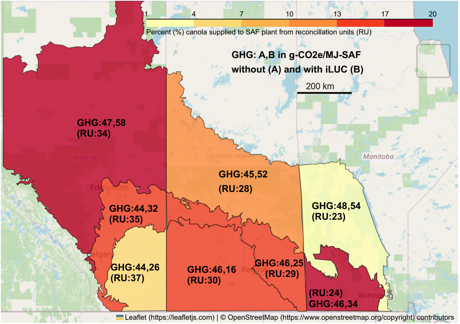Fig. 10 Choropleth shows the canola availability (in %) and LC-GHG emissions of SAF produced from each reconciliation unit (RU) for the best profitability scenario at 25% feedstock accessibility criteria. The LC-GHG emissions are denoted as “GHG: A, B”, where ‘A’ indicates LC-GHG emissions (g CO₂e per MJ-SAF) excluding the land-use (LU) and land-management changes (LMC) and ‘B’ indicates LC-GHG emissions including LU and LMC.

The RU with the largest canola availability is also the region with the largest LC-GHG emissions. RU-34 has nearly 20% of the available canola but has LC-GHG emissions of 58 g CO₂e per MJ, suggesting that plants in the northern Alberta region would likely have a larger carbon footprint, because they are more likely to source high-carbon intensity canola. The higher LC-GHG emissions in RU-34 is due to the legacy emissions associated with the conversion of forest land to cropland over the years.⁵⁷ The canola-derived SAF from RU-23 has an LC-GHG emission of 54 g CO₂e per MJ, nearly as high as RU-34, but the total available canola in this upper Manitoba region is just 2%, and therefore unlikely to affect the national average LC-GHG emissions. RU-30, on the other hand, has the lowest LC-GHG emissions with just 16 g CO₂e per MJ – almost 72% lower than LC-GHG emissions from RU-34, and has about 15% of available canola. The very low emissions in this region are due to sustainable land management practices such as near-zero direct land-use change, reduction in summer fallow, and improved tillage practices.⁵⁷

The optimal plant sites identified are likely to collect canola from multiple RUs depending on the location, leading to weighted average LC-GHG emissions from different RUs. Fig. 11 shows optimal SAF plant locations and the canola collected from different reconciliation units (RUs) in the best profitability scenario for a collection distance of 200 km and a 25% feedstock accessibility guideline. The canola sourced from each reconciliation unit is highlighted in different colours to differentiate the source of canola supplied from multiple RUs.

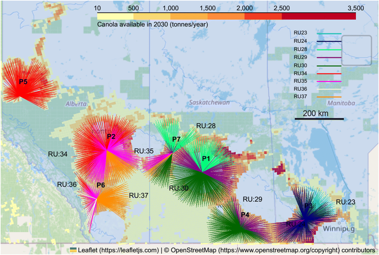Fig. 11 Canola from different reconciliation units (RU: 23–37) allocated to optimal SAF locations (P1–P7) in the best profitability scenario for a 25% feedstock accessibility guideline. The colour of the lines indicates the canola produced from different reconciliation units. RU 23: deep sky blue, RU 24: dark blue, RU 28: spring green, RU 29: purple, RU 30: dark green, RU 34: red, RU 35: magenta, RU 36: beige and RU 37: dark orange. The RU numbers are marked close to the colours for easy identification. The origin of the lines indicates the source of canola and the converging point indicates the SAF plant site.

We have estimated the LC-GHG emissions of the SAF produced from the optimal location identified in our study and identified locations with the lowest LC-GHG emissions. Table 8 shows the life cycle GHG emissions of the canola-derived SAF obtained from the optimal locations identified in the best profitability scenario. Location P6 stands out as having the highest LC-GHG (58 g CO₂e per MJ) emissions due to its exclusive reliance on RU-34. The three largest and most profitable locations (P1–P3) exhibit moderate emissions (32–40 g CO₂e per MJ), with lowest emissions being attributed to some of the smaller and less profitable locations (P4, P5, P7, 20–32 g CO₂e per MJ). The lack of correlation between profitability and associated emissions suggests a potential role for targeted policy support to nudge facilities toward prioritizing environmentally preferable locations.

Table 8 Life cycle GHG emissions of canola-derived SAF from optimal locations (P1–P7) identified in the maximum profitability scenario for a 25% feedstock accessibility guideline. The table gives a split of the canola derived from multiple reconciliation units for each optimal location

Optimal SAF location	LC-GHG of SAF (g CO2e per MJ)	Percent canola from reconciliation units (RU)
		RU-23	RU-24	RU-28	RU-29	RU-30	RU-34	RU-35	RU-37
LC-GHG	—	54	34	52	25	16	58	32	26
P1	32			35%	35%	30%
P2	40						35%	55%	10%
P3	36	5%	90%		4%
P4	20				43%	57%
P5	29						4%	41%	55%
P6	58						100%
P7	32			35%	21%	33%		9%	2%

---

4. Discussion and policy implications

4.1. Canola availability and site selection

The total production of canola expected in 2030 is conservatively estimated at 24.7 MT. Out of 24.7 MT, 9.5 MT is allocated to existing domestic uses, and nearly 15.2 MT (62%) can be captured for new domestic uses before exports. Most of the available canola is in the northern Alberta, northern Saskatchewan, and southern Manitoba regions. It is interesting to note that even after removing current canola consumption by existing industries, the best locations with the greatest access to canola are close to existing canola crush plants and biodiesel plants (ESI,† Section S10). Most of the existing plants are in the middle of canola production regions and have access to canola from many directions.

Based on our site selection analysis, which includes various infrastructure criteria, there are about 320 potential sites suitable for canola-derived SAF, reduced from over 6800 sites based on canola availability alone. Restricting the number of potential sites significantly reduces the computation time required in the optimization step. The resulting sites are evenly distributed between Alberta, Saskatchewan, and Manitoba. Among the various site selection criteria applied, the use of remoteness index effectively reduced the unsuitable sites by nearly 30%, compared to the baseline 6800 sites. The criterion specifying access to rail & road infrastructure eliminated 65% of the 6800 potential sites, suggesting that the rail/road criteria is a key limitation. Finally, proximity to population centres eliminated 14% of the 6800 sites; prior criteria had already eliminated remote sites. Thus, all site selection criteria proposed here play a meaningful role narrowing the list of viable sites. Most of the potential locations in Alberta are situated close to major highways (Hwy 2 and Hwy 16) connecting Calgary–Edmonton–Lloydminster in Alberta. In Saskatchewan, the potential locations are clustered near Saskatoon, Regina, and highways (Hwy 16, and Hwy 1). In Manitoba, the potential locations are close to Winnipeg, Brandon and the inter-provincial highway (Hwy 16 and PTH 1) connecting to Saskatchewan.

4.2. National canola SAF potential and optimal locations

If a facility is not constructed at a potential site, it could be argued as a lost opportunity to produce SAF and, ultimately, would reduce national SAF potential. The financial sector's guidelines on feedstock accessibility have a large influence on whether a plant is constructed at a particular location. According to biofuel investors, it is unrealistic to assume that more than 50% of the available feedstocks in a canola producing region can be captured by new users. A low feedstock accessibility, e.g., 25% of feedstock available, selected in a biofuel feasibility study suggests a lower risk for investors regarding feedstock supply, and a higher assumed level of feedstock accessibility, e.g., 50%, suggests a higher risk of feedstock supply, and subsequently, a price risk in the event of adverse events. Investors might be willing to consider a higher feedstock accessibility if the risk is reduced via an effective feedstock supply chain, which can be done by increasing the connectivity of supply from the canola producing regions to potential industrial locations. Currently, about 99% of the grain elevators in Canada are connected via a single railway line for delivery to ports or industrial facilities. Almost 55% of the rail cars do not deliver grain products on time, and almost 40% of the rail cars are delivered four weeks late.⁷³ Improving supply chain connectivity could increase commercial users’ access to canola, allowing a higher assumed level of feedstock accessibility in feasibility studies and a lower risk for investors.

We found that Canada can produce about 1–1.8 billion litres of canola SAF annually, depending on the feedstock accessibility criteria assumed in the model (25–45%). Canola has the potential to contribute to 12–21% of Canada's 2019 jet fuel consumption of 8.7 billion litres.⁷⁴ Among the three provinces, annually, Saskatchewan and Alberta can supply about 780 and 720 million litres, respectively, and Manitoba can supply about 330 million litres. The sensitivity analysis feedstock accessibility suggests that increasing the canola accessibility is unlikely to change the optimal locations identified, and therefore, future yield increases, if geographically uniform, may not alter the optimal locations in Canada. The most profitable locations have access to large amounts of canola, suggesting that economies of scale matter, and it is crucial for biofuel producers to choose locations with ample access to feedstock. In the most profitable scenario, about 7–8 potential SAF plants are possible in Canada, with a utilization of about 6 MT of canola for renewable fuels. Any further allocation of canola for fuels, i.e., more than 50% of available canola for SAF, can potentially increase the cost of canola and induced land-use change GHG emissions, which needs to be considered when estimating profitability and life cycle GHG emissions.

Interestingly, at the time of writing this manuscript, the Canadian Council of Sustainable Aviation Fuel (C-SAF) published their C-SAF Roadmap highlighting the potential feedstock availability for SAF production by 2030 in Canada.⁶³ The C-SAF estimates for canola-derived SAF were between 600 and 1000 ML, depending on the assumptions regarding canola accessibility. The C-SAF estimates for SAF production from canola were lower than our estimates (1000–1800 ML) because the model assumed that only the current exported canola can be captured for SAF, and did not account for the projected increase in canola production by 2030.

Unlike US Inflation Reduction Act (IRA), Canada does not have a direct federal production incentive for every gallon of SAF produced locally. However, inclusion of blending mandates in the BC's low carbon fuel standard and ability of SAF to generate low carbon credits in the Canadian Clean Fuel Regulations (CFR) could encourage domestic SAF production. In British Columbia, there is a SAF volumetric blending mandate of 1% in 2028, 2% in 2029, and 3% by 2030 and subsequent compliance periods.⁷⁵ It also requires a reduction in in carbon intensity of SAF by 2% compared to fossil jet fuel in 2026 increasing to 10% by 2030.⁷⁶ There are no specific policies that are aimed at SAF in the 2022 Canadian Clean Fuel Regulations.⁷⁷ However, there is a provision to generate credits for SAF as a voluntary opt-in. Also, the federal government, through the Treasury Board Canada, made a provision to procure the low-carbon fuel for federal air and marine fleets.⁶³ Since SAF is 2–5 times more expensive than conventional jet fuel,⁷⁸ it is not viable without incentives. In the case of Canada, incentives are required to avoid losing canola to SAF production in US due to their more favourable incentives. Thus, the premise of this study is to assess SAF potential under the assumption that sufficient incentives will be in place to enable the market to take root in Canada; as such this study uses a generalized and larger SAF incentive rather than attempting to capture the nuance of the current patchwork of related policies.

4.3. LC-GHG emissions

There was a large variation in LC-GHG emissions of canola-derived SAF from the potential locations when land-use change (LU) and land-management changes (LMC) were considered. ICAO suggests that direct land-use change emissions (DLUC) should be included if the land was converted from forest to cropland after 2008.⁷⁹ Therefore, canola produced from recent croplands would not be selected, to avoid carrying over legacy GHG emissions for SAF. Among the available canola in Canada, nearly one-fifth is in the RU-34 region in northern Alberta, which also has the highest life cycle GHG emissions of about 58 g CO₂e per MJ for the canola-derived SAF. Hence, careful judgment needs to be taken based on how much the LC-GHG emissions are likely to affect CORSIA obligations or carbon pricing in Canada before selecting a location for a SAF plant in these regions. The southern Saskatchewan region has about 32% of the available canola with the lowest LC-GHG emissions of about 16 g CO₂e per MJ-SAF and 25 g CO₂e per MJ-SAF in the RU-30 and RU-30 regions. In particular, location P4, close to Weyburn in southern Saskatchewan, has the lowest LC-GHG emissions of 20 g CO₂e per MJ-SAF.

The LC-GHG emissions from the SAF produced from the optimal locations identified in the best profitability scenario ranges from 20 (P4) and 58 (P6) g CO₂e per MJ-SAF. The differences in LC-GHG emissions between locations can also influence the site selection by industries. For a volumetric energy density of 35 MJ per L,⁸⁰ and carbon price of 170 C$ per tonne in 2030,⁷¹ the difference in cost due to the life cycle carbon emissions can be as high as 23 cents per L. The additional cost of 23 cents per L is 40% of the jet fuel price (56.6 cents per L) and 38% of the incentives (60 cents per L) used in this study (ESI,† Section S12). Policymakers could, therefore, consider offering incentives to encourage industries to produce SAF from the available canola in the low life cycle GHG regions to reduce the national average GHG emissions in the aviation sector. However, in doing so, it may force other industries to use canola with higher crop emissions, offsetting the benefit of using low carbon-intensity canola for biofuels.

5. Summary and conclusion

We have proposed a framework for estimating the biofuel potential and, as a case study, estimated the national canola SAF potential in Canada. Our work expanded upon the current understanding of canola supply chain analysis by considering HEFA-based SAF and incorporated rigorous site selection metrics such as the remoteness index, industry guidelines for feedstock accessibility, and empirical information on proximity to rail, road, and population centres. Our analysis suggests that Canada can produce about 1–1.8 billion litres of SAF from canola by 2030, which translates to 12–21% of Canada's jet fuel consumption in 2019. The optimal sites for SAF production are concentrated near major cities/towns and are located near existing biofuel plants, despite competition for feedstock. Most of the potential locations are situated close to major highways (Hwy 2 and Hwy 16) connecting Calgary–Edmonton–Lloydminster, Hwy 16 and Hwy 1 in Manitoba (sites close to Winnipeg, Brandon) and the inter-provincial highway (Hwy 16 and PTH 1) connecting Saskatchewan. The average LC-GHG emissions of the SAF produced are expected to range between 20–58 g CO₂e per MJ-SAF.

Overall, we conclude that there is a limit on the amount of canola produced in Canada that can be made available for biofuel production, due to project risks, economic constraints, and competing demands via export markets. The canola supply chain connectivity can severely restrict SAF potential. Increasing the supply of canola for SAF production is contingent upon improved transportation connectivity between canola production and biofuel production centers and from the biofuel production facilities to refineries and terminals where the SAF would be blended. Most of the proposed SAF plants in Canada are situated within existing major industrial complexes or strategically positioned along transportation routes, including ports, where canola shipments can be intercepted. With the major contribution of feedstock costs to the overall biofuel production cost, optimal locations for SAF plants will be determined access to low cost canola and by access to existing industrial infrastructure that reduces capital and production costs. From a policy perspective, the feedstock cost risk could be mitigated (in part) by devising incentives linked to feedstock prices. In particular, incentives that increase during short-term price shocks would help to manage risk.

The financial attractiveness of the export market is partly driven by the difference in incentives between the US and Canada, posing an impediment to the development of a domestic SAF market. Within Canada, regional differences in the CI of SAF can influence decisions for citing plants, apart from other site selection criteria. The overall production potential using canola is significant, but not sufficient to meet total potential demand. Therefore, it is essential to apply the framework to assess SAF potential from other feedstocks such as soy, municipal solid waste (MSW), forest and agricultural residues.

Abbreviations

NPV	Net present value
ROI	Return on investment
BIMAT	Biomass inventory mapping and analysis tool
MLPY	Million litres per year
CAPEX	Capital expenditure
OPEX	Operating expenditure
MTPY	Million tonnes per year
IRR	Internal rate of return
ROI	Return-on-investment
MSW	Municipal solid waste
SI	Supplementary information

Author contributions

Praveen Siluvai Antony: conceptualization, methodology, formal analysis, investigation, data curation, writing – original draft, and visualization. Caroline Vanderghem: data curation and resources. Heather MacLean: methodology, writing – review & editing, and funding acquisition, Bradley Saville: conceptualization, methodology, supervision, writing – review & editing, and funding acquisition, Daniel Posen: conceptualization, methodology, writing – review & editing, supervision, project administration, and funding acquisition.

Conflicts of interest

There are no conflicts to declare.

Acknowledgements

The authors would like to acknowledge the financial support from Transport Canada's Clean Transport System – Research and Development Program (CTS-R&D) grant on “Life cycle environmental and economic evaluation of aviation biofuels in Canada”. The authors would like to thank Agriculture and Agri-Food Canada staff members David Lee, and Alyssa Klein for providing the historical Canola production geospatial data, Darrel Cerkowniak for sharing the shapefile for Reconciliation unit and soil map of Canada, and Lawrence Townley-Smith for data requests. We also would like to thank Prof. Michael Griffin from Carnegie Mellon University and Jon Obnamia from Transport Canada for their input during discussions.

References

1. ICAO, Envisioning a “zero climate impact” international aviation pathway towards 2050: how governments and the aviation industry can step-up amidst the climate emergency for a sustainable aviation future, 2019.
2. ICAO, Sustainable Aviation Fuels Guide. ICAO. International Civil Aviation Organization, 2016.
3. E. Asmelash, F. Boshell and G. Castellanos, Reaching Zero With Renewables. The International Renewable Energy Agency (IRENA), Abu Dhabi, International Renewable Energy Agency (IRENA), 2021, p. 96.
4. Navius Research, Achieving net zero emissions by 2050 in Canada: An evaluation of pathways to net zero, 2021.
5. M. Shehab, K. Moshammer, M. Franke and E. Zondervan, Analysis of the Potential of Meeting the EU's Sustainable Aviation Fuel Targets in 2030 and 2050, Sustainability, 2023, 15(12), 9266 , https://www.mdpi.com/2071-1050/15/12/9266.
6. H. Mohammadi, Decarbonizing long-distance transport. BC-SMART, 2022, https://c-saf.ca/.
7. D. M. Johnson, T. L. Jenkins and F. Zhang, Methods for optimally locating a forest biomass-to-biofuel facility, Biofuels, 2012, 3(4), 489–503.
8. P. T. Lautala, M. R. Hilliard, E. Webb, I. Busch, J. Richard Hess and M. S. Roni, et al., Opportunities and Challenges in the Design and Analysis of Biomass Supply Chains, Environ. Manage., 2015, 56(6), 1397.
9. L. Martinez-Valencia, M. Garcia-Perez and M. P. Wolcott, Supply chain configuration of sustainable aviation fuel: Review, challenges, and pathways for including environmental and social benefits, Renewable Sustainable Energy Rev., 2021, 152, 111680.
10. D. S. Gonzales and S. W. Searcy, GIS-based allocation of herbaceous biomass in biorefineries and depots, Biomass Bioenergy, 2017, 97, 1–10,  DOI:10.1016/j.biombioe.2016.12.009.
11. S. Leduc, F. Starfelt, E. Dotzauer, G. Kindermann, I. McCallum and M. Obersteiner, et al., Optimal location of lignocellulosic ethanol refineries with polygeneration in Sweden, Energy, 2010, 35(6), 2709,  DOI:10.1016/j.energy.2009.07.018.
12. P. O. Lemire, B. Delcroix, J. F. Audy, F. Labelle, P. Mangin and S. Barnabé, GIS method to design and assess the transportation performance of a decentralized biorefinery supply system and comparison with a centralized system: case study in southern Quebec, Canada, Biofuels, Bioprod. Biorefin., 2019, 13(3), 552.
13. B. Sharma, S. Birrell and F. E. Miguez, Spatial modeling framework for bioethanol plant siting and biofuel production potential in the U.S, Appl. Energy, 2017, 191, 75–86,  DOI:10.1016/j.apenergy.2017.01.015.
14. M. K. Delivand, A. R. B. Cammerino, P. Garofalo and M. Monteleone, Optimal locations of bioenergy facilities, biomass spatial availability, logistics costs and GHG (greenhouse gas) emissions: A case study on electricity productions in South Italy, J. Cleaner Prod., 2015, 99, 129,  DOI:10.1016/j.jclepro.2015.03.018.
15. L. Panichelli and E. Gnansounou, GIS-based approach for defining bioenergy facilities location: A case study in Northern Spain based on marginal delivery costs and resources competition between facilities, Biomass Bioenergy, 2008, 32(4), 289–300.
16. A. Sultana and A. Kumar, Optimal siting and size of bioenergy facilities using geographic information system, Appl. Energy, 2012, 94, 192–201,  DOI:10.1016/j.apenergy.2012.01.052.
17. K. Natarajan, S. Leduc, P. Pelkonen, E. Tomppo and E. Dotzauer, Optimal locations for second generation Fischer Tropsch biodiesel production in Finland, Renewable Energy, 2014, 62, 319,  DOI:10.1016/j.renene.2013.07.013.
18. N. Parker, Q. Hart, P. Tittmann and B. Jenkins, National Biofuel Supply Analysis. Prepared for the Western Governor's Association, Contract, 2011, 3.
19. T. L. Jenkins, E. Jin and J. W. Sutherland, Effect of harvest region shape, biomass yield, and plant location on optimal biofuel facility size, Forest Policy and Economics, 2020, 111, 102053,  DOI:10.1016/j.forpol.2019.102053.
20. E. G. O’Neill, R. A. Martinez-Feria, B. Basso and C. T. Maravelias, Integrated spatially explicit landscape and cellulosic biofuel supply chain optimization under biomass yield uncertainty, Comput. Chem. Eng., 2022, 160, 107724,  DOI:10.1016/j.compchemeng.2022.107724.
21. M. P. Wolcott, Alternative Jet Fuel Supply Chain Analysis, Washington State University, 2020.
22. B. Saville Feasibility Study for a Biodiesel Refining Facility in the Regional Municipality of Durham Prepared for: Regional Municipality of Durham, BBI Biofuels Canada, Durham, Canada, 2006.
23. R. T. L. Ng and C. T. Maravelias, Design of Cellulosic Ethanol Supply Chains with Regional Depots, Ind. Eng. Chem. Res., 2016, 55(12), 3420.
24. N. Zarrinpoor and A. Khani, Designing a sustainable biofuel supply chain by considering carbon policies: a case study in Iran, Energy Sustainability Soc., 2021, 11(1), 1–22,  DOI:10.1186/s13705-021-00314-4.
25. F. Zhang, D. Johnson, M. Johnson, D. Watkins, R. Froese and J. Wang, Decision support system integrating GIS with simulation and optimisation for a biofuel supply chain, Renewable Energy, 2016, 85, 740,  DOI:10.1016/j.renene.2015.07.041.
26. Statistics Canada. Index of Remoteness, 2020, https://www150.statcan.gc.ca/n1/pub/17-26-0001/172600012020001-eng.html.
27. B. Saville, Personal communication with biofuel industry experts, 2020.
28. S. Sokhansanj, A. Kumar and A. F. Turhollow, Development and implementation of integrated biomass supply analysis and logistics model (IBSAL), Biomass Bioenergy, 2006, 30, 838–847.
29. Statistics Canada, www.12.statcan.gc.ca, 2019, Census Profile, 2016 Census, pp. 1–2, https://www12.statcan.gc.ca/census-recensement/2016/dp-pd/prof/index.cfm?Lang=E.
30. Statistics Canada, Road network Canada, Government of Canada, 2019.
31. DMTI Spatial Inc, Markham Ontario, Canada, 2014, CanMap Rail, https://geo.scholarsportal.info/#r/details/_uri@=2680653796$DMTI_2014_CanMapRAIL_RL_CAN.
32. F. Zhang, D. M. Johnson and J. W. Sutherland, A GIS-based method for identifying the optimal location for a facility to convert forest biomass to biofuel, Biomass Bioenergy, 2011, 35(9), 3951,  DOI:10.1016/j.biombioe.2011.06.006.
33. EPSG, Canada Atlas Lambert – EPSG:3979, 2009, https://epsg.io/3979.
34. Agriculture and Agri-Food Canada, Canada. ISO 19131 Biomass Inventory Mapping and Analysis Tool Business Data – Data Product Specification, Government of Canada, 2020, https://open.canada.ca/data/en/dataset/1a759d95-3008-4078-87af-5bb1bdf657b3.
35. Canola Council of Canada, Canadian canola export statistics, 2021, https://www.canolacouncil.org/markets-stats/exports/.
36. Canola Council of Canada, Canola industry in Canada: from farm to global markets, 2021, https://www.canolacouncil.org/about-canola/industry/.
37. Biodiesel Magazine, Canadian Biodiesel Plants. Biodiesel magazine, 2020, https://www.biodieselmagazine.com/plants/listplants/Canada/.
38. J. Véronique Barthet, Quality of western Canadian Canola 2019, Winnipeg, Canada: Canadian Grain Commission, 2019, pp. 1–30.
39. AGCanada, Bunge to expand southern Man. canola crush plant, 2010, https://www.agcanada.com/daily/bunge-to-expand-southern-man-canola-crush-plant-2.
40. AGCanada, Dreyfus’ Yorkton canola crush plant status still unclear, 2014, https://www.agcanada.com/daily/dreyfus-yorkton-canola-crush-plant-status-still-unclear.
41. Cargill, 2021, Cargill industrial locations. https://www.cargillag.ca/locations.
42. Richarson Inc, Richardson, 2016, Richardson invests $120 million to upgrade Lethbridge canola plant, https://www.richardson.ca/richardson-invests-120-million-to-upgrade-lethbridge-canola-plant-2/.
43. Rod N. Reuters, Canadian Bioenergy, ADM mull Alberta biofuel plant, 2009, https://www.reuters.com/article/canada-us-biofuel-idCATRE5375NH20090408.
44. D. Brewin The Processing Plant Location Problem: The Case of Canola Crushing The Processing Plant Location Problem: Canola Crushing in Western Canada, in: Canadian Agricultural Economics Society Joint Annual Meeting, Vancouver, British Columbia, 2015, p. 24, https://www.researchgate.net/publication/273456400_The_Processing_Plant_Location_Problem_The_Case_of_Canola_Crushing_in_Western_Canada.
45. Agriculture and Agri-Food Canada, Open Governmental Portal, Grain Elevators in Canada, 2023, https://open.canada.ca/data/en/dataset/05870f11-a52a-4bf4-bc15-910fd0b8a1a3.
46. J. McMillan, S. Jack and T. Geoffrey, Webinar Series IEA Bioenergy: Sustainable Aviation Fuel/Biojet Technologies - Commercialization Status, Opportunities, and Challenges, British Columbia, Canada: IEA Bioenergy, 2021, https://www.ieabioenergy.com/blog/publications/iea-bioenergy-webinar-sustainable-aviation-fuel-biojet-technologies-commercialisation-status-opportunities-and-challenges/.
47. P. L. Chu, C. Vanderghem, H. L. MacLean and B. A. Saville, Financial analysis and risk assessment of hydroprocessed renewable jet fuel production from camelina, carinata and used cooking oil, Appl. Energy, 2017, 198, 401,  DOI:10.1016/j.apenergy.2016.12.001.
48. M. McAdams and P. Argyropoulos, The Future of Advanced Renewable Jet Fuel is Bright, Advanced Biofuels Association, 2021, pp. 1–24, https://www.acs.org/acswebinars.
49. A. Alasia, F. Bédard, J. Bélanger, E. Guimond, C. Penney and S. Canada, et al., Measuring remoteness and accessibility - A set of indices for Canadian communities. Statistics Canada – Catalogue no. 18-001-X, Statistics Canada, 2017, pp. 1–43.
50. D. A. Camenzind, Supply Chain Analysis For Sustainable Alternative Jet Fuel Production From Lipid Feedstocks In The U.S. Pacific Northwest, Washington State University, 2018.
51. LMC International, The Economic Impact of Canola on the Canadian Economy: 2020 Update, vol. 1, Winnipeg, Canada: Canola Council of Canada, 2020, https://www.canolacouncil.org/download/131/economic-impact/17818/economic-impact-report-canada_december-2020.
52. SimpleMaps, Canada Cities Database, 2020, https://simplemaps.com/data/canada-cities.
53. L. G. Pereira, H. L. MacLean and B. A. Saville, Financial analyses of potential biojet fuel production technologies, Biofuels, Bioprod. Biorefin., 2017, 11(4), 665.
54. U.S. Department of the Treasury, 2024, U.S. Department of the Treasury, IRS Release Guidance to Drive American Innovation, Cut Aviation Sector Emissions, https://home.treasury.gov/news/press-releases/jy1998.
55. W. F. Torrey, An Analysis of the Operational Costs of Trucking: A 2020 Update. 950 N. Glebe Road, Suite 210 Arlington, Virginia 22203, USA: American Transportation Research Institute, 2020, p. 53.
56. Transcourt Truck Leasing Inc, Transcourt Tank Leasing, How much gas does a tanker truck hold? Ontario, Canada, 2018, pp. 4–7, https://transcourt.com/blog/how-much-gas-does-a-tanker-truck-hold/.
57. J. A. Obnamia, H. L. MacLean and B. A. Saville, Regional variations in life cycle greenhouse gas emissions of canola-derived jet fuel produced in western Canada, GCB Bioenergy, 2020, 12(10), 818.
58. J. Sabrsula, Site Selection for the Biofuels Industry. Trade & Industry Development. 2007, pp. 1–3. https://www.tradeandindustrydev.com/industry/alternative-energy-fuels/site-selection-biofuels-industry-485.
59. Green Car Congress. Green Car Congress, 2019. HollyFrontier to build $350M renewable diesel unit at Artesia refinery; 125M gallons/year, https://www.greencarcongress.com/2019/12/20191209-hollyf.html.
60. Reuters, 2020, 1 HollyFrontier to convert oil refinery into renewable diesel plant, https://www.reuters.com/article/us-hollyfrontier-refining-cheyenne-idUSKBN2383LF.
61. US Department of Agriculture. USDA Website. 2018. Canola production in Canada in 2018. https://ipad.fas.usda.gov/rssiws/al/crop_production_maps/Canada/Canada_Canola.png.
62. Canadian Oilseed Processors Association. Overview of Canada's Oilseed Processing Sector, 2018.
63. B. Allan, J. Goldman, G. Tauvette, P. Leung, J. Rohl and D. Vincent, et al., The C-SAF Roadmap Building a feedstocks-to-fuels SAF supply chain in Canada Authorship team Facilitation and Strategy, 2023.
64. J. Yang, Z. Xin, Q. He, K. Corscadden and H. Niu, An overview on performance characteristics of bio-jet fuels, Fuel, 2019, 237, 916.
65. K. Rispoli, Life cycle and supply assessment of aviation biofuels in the Canadian context, 2014.
66. Edmonton International Airport Authority. Edmonton International Airport: Master Plan 2010–2035 Executive Summary, 2011.
67. InterVISTAS, 2020 Economic Impact Study Final Report: Winnipeg James Armstrong Richardon International Airport (YWG). Winnipeg, Canada: Winnipeg Airports Authority, 2020, p. 56.
68. Ausenco Sandwell company GAI, Evaluation of Fuel Delivery Options. Richmond, Brisith Columbia: Vancouver Airport Fuel Facilities Corporation (VAFFC), 2011, p. 91.
69. ImperialOil, ImperialOil News, 2021, Imperial to produce renewable diesel at Strathcona refinery, https://news.imperialoil.ca/news-releases/news-releases/2021/Imperial-to-produce-renewable-diesel-at-Strathcona-refinery/default.aspx.
70. Rod Nickel. Reuters. 2022, Federated Co-op, AGT to build C$360-mln Canadian canola crush plant|Reuters, https://www.reuters.com/business/energy/federated-co-op-agt-build-c360-mln-canadian-canola-crush-plant-2022-01-17/.
71. Government of Canada. Clean Fuel Regulations: Canada Gazette, Part 1, Volume 154, Number 51, 2021, https://gazette.gc.ca/rp-pr/p1/2020/2020-12-19/html/reg2-eng.html.
72. ICAO, Life Cycle Emissions of Sustainable Aviation Fuels, 2022, https://www.icao.int/environmental-protection/pages/SAF_LifeCycle.aspx.
73. Canadian Canola Growers Association, Agriculture can grow our economy but rail service must respond to market demand, 2015.
74. Statistics Canada, Civil aviation fuel consumption from Canadian air carriers, 2023, https://www150.statcan.gc.ca/t1/tbl1/en/tv.action?pid=2310026701.
75. Government of British Columbia, Low Carbon Fuel Standard: Aviation Fuel Regulation Intentions Paper, 2023, https://www2.gov.bc.ca/assets/gov/farming-natural-resources-and-industry/electricity-alternative-energy/transportation/renewable-low-carbon-fuels/aviation_intentions_paper.pdf.
76. E. Voegele, British Columbia revamps low carbon fuel regs, requires SAF. Biomass Magazine, 2023, https://biomassmagazine.com//articles/british-columbia-revamps-low-carbon-fuel-regs-requires-saf.
77. H. Mohammadi, Decarbonizing the Aviation Sector, 2023.
78. IAT, Unlocking geographical constraints on the global SAF market through a robust SAF accounting framework, 2023.
79. ICAO, CORISA sustainability criteria for CORSIA eligible fuels. ICAO, 2019, pp. 1–3.
80. US DOE, Sustainable Aviation Fuel: Review of Technical Pathways Report, 2020.

---

Footnote

† Electronic supplementary information (ESI) available. See DOI: https://doi.org/10.1039/d3ya00579h

---