Particulate matter in a lockdown home: evaluation, calibration, results and health risk from an IoT enabled low-cost sensor network for residential air quality monitoring

Abstract

Exposure to atmospheric particulate matter is associated with a wide array of health impacts. Whilst ambient air pollution exposure is widely discussed both within the scientific literature and media, indoor exposure to pollutants has received less attention. However, humans spend a large amount of time in indoor environments, which increased significantly during the Covid-19 pandemic. This paper tests the application of a low-cost Internet of Things (IoT) enabled indoor sensor network to provide a relative assessment of variations in PM in a lockdown home. The paper validates the low cost, IoT approach via sensor corrections and testing before assessing particulate concentrations for a ∼7 week period within a typical suburban home in the UK. With the caveat that data from low-cost sensors are at best indicative, it was found that particulate matter concentrations in multiple rooms exceeded both 2021 and 2005 WHO Global Air Quality Guidelines, when extrapolated to annual exposure levels, despite relatively low ambient concentrations. Concentrations peaked at 488 μg m⁻³ (PM_2.5) when cooking was occurring within the home.

---

Environmental significance

Exposure to particulate matter can have a wide array of health impacts. Humans spend 60–90% of their time indoors and the modal shift towards hybrid working is increasing the time people spend in residential settings (Guyot et al., 2018,³ Domínguez-Amarillo et al., 2020 (ref. 4)). Capturing exposure to particulates within the home can be challenging-studies can be intrusive on residents lives and can be limited by the expense of monitoring equipment. Low-cost sensor networks provide novel opportunity to monitor pollutants within homes, yet often their performance is questioned due to their price point. This paper presents the successful deployment of a low-cost PM sensor network within a home, highlighting concentrations by room and activity.

1 Introduction

Globally, 1 in 10 deaths are estimated to be associated with pollution-induced disease, contributing to 7 million premature deaths worldwide each year.^1,2 Whilst ambient air pollution exposure is the predominant focus of research efforts, humans typically spend 60–90% of their time indoors. Time activity patterns have also changed in recent years due to the Covid-19 pandemic, which led to increased time spent in domestic indoor environments, with a subsequent modal shift to home and hybrid working schedules in specific employment sectors.^3,4 Away from employment and working habits, typical residential activities such as cooking, sleeping and cleaning within the home are also associated with exposure to indoor pollutants. WHO suggest Air Quality Guidelines for key pollutants including PM_2.5 and PM₁₀. These guidelines are evidence based and are designed to suggest levels at which evidence for impacts on health have been reported.⁵ For this reason, this study uses these guidelines for comparing particulate concentrations.

Low-cost air quality sensors provide a novel opportunity for monitoring relative concentrations of particulate matter at previously unattainable spatial resolution, and the Internet of Things (IoT) allows for the development of indoor air quality (IAQ) networks.^6,7 There are a number of existing studies that assess indoor particulate matter (PM) pollution, however a frequent limitation of these studies is monitoring is limited to only 1 or 2 locations within a property (often a kitchen or main living area).^4,8–21 Shen et al. (2021)³⁵ reported a comprehensive multi-room study with multiple sensors, yet this was limited to PM_2.5 (particles with aerodynamic diameters <2.5 μm) as the sensors were not calibrated for the PM₁ & PM₁₀ (particles with diameters <1 μm and <10 μm respectively) fractions that they also monitored. Few previous studies have used IoT networks for monitoring, and those that did, tended to use IoT networks that are reliant on gateway or WiFi technology thus limiting deployment.^6,15,22

Whilst ambient corrections and calibrations for indicative monitoring devices are starting to become established within the scientific literature, there remains a need for this to be adapted to suit the nuances of indoor monitoring environments. Ambient correction methods are usually based on co-location with a reference grade instrument, taking into account the impact of humidity on hygroscopic particles, and often using ‘buddy’ matching or data validation from nearby ambient regulatory monitors. However, indoor air samples are problematic as indoor humidity levels are typically lower than ambient and indoor environments do not typically have regulatory monitors for comparison outside of a laboratory environment for buddy matching. Some studies have attempted to develop indoor calibrations methods to varying success, but tend to base corrections on a co-location with a reference instrument exposed to a specific particulate source which is not representative of the array of PM sources or activities that normally occur within a home.^23–25 The purpose of this study was to address these research gaps by deploying an IoT sensor network of 5 low-cost sensors (AltasensePM-compromised of an IoT enabled Plantower PMS5003) across a single residential property during a period of coronavirus restrictions, accounting for different rooms and the outside/ambient environment. Analysis is driven by the following foci:

(1) Validate the application of IoT low-cost sensor networks for indoor air quality, including the development of a method for correcting and validating low-cost data within an indoor setting.

(2) Evaluate the impact of human activity and different sources on relative real-time PM levels throughout a residential property, inclusive of indoor : outdoor ratios.

2 Background

2.1 The problem of indoor particulate matter

PM pollution is of public health concern due to the wide variety of health impacts its inhalation can cause. There are numerous sources of PM and with varying PM composition and health impacts of exposure are widespread, including cardio-vascular and respiratory morbidity and mortality.^26,27 The World Health Organisation (WHO) recommend air quality guidelines however historically these focused on ambient concentrations. IAQ advice was introduced in 2010, although they didn't specify guidelines for each PM size fraction within the home unlike the 2005 ambient guidelines which suggested guideline concentrations for different PM size fractions.^28,29 In the most recent WHO update in late 2021, the ambient guidelines for each size fraction were also recommended to be applicable to indoor environments too.⁵ This means that historically, despite the major health implications of PM, the domestic environment in which people spend the majority of their time is overlooked. This was highlighted further by the impact of coronavirus restrictions in 2020/21 which increased the amount of time people spent at home via work from home orders; the closure of social/entertainment environments such as restaurants and gyms and social contact restrictions. This provided both an opportunity to study indoor air quality in new detail, looking at the increased exposure and activity within the home but also challenges as access to infrastructure and instruments to support a study were limited by the pandemic restrictions.

There are many sources of PM within the home. Firstly, ambient (outdoor) PM pollution can infiltrate the home however these particles tend to have a limited size distribution as the more coarse and ultrafine particles (UFPs) are typically removed during transmission.^19,30 In older properties, infiltration occurs via leakage throughout the property, or by manual ventilation introduced by opening and closing windows and doors, however as building standards have evolved, properties have become increasingly air tight to increase energy efficiency.³¹ These newer properties tend to rely on mechanical ventilation such as fans and extractors, yet these are not always as effective as promised and can even generate their own pollutants from running (i.e. mechanical wear).^32,33 Secondly, everyday activities/interactions within the home can generate and influence PM concentrations, such as daily household activity from household chores and resuspension from movement. Prominent indoor sources include cooking and smoking however other sources such as candles, cleaning, vacuuming, humidifiers, combustion of solid fuels and resuspension have also been discussed within literature.^8,30,34–37 The prominence of the sources will vary both spatially and seasonally along with the indoor : outdoor ratio (I : O), and generally it is found that in winter PM from indoor sources contributes proportionately more and is higher in magnitude.^11,38

People spend on average 1/3 of their life asleep-yet IAQ studies that assess bedroom and sleeping period particulates are limited to high income settings.^39,40 Less than one quarter (23%) of studies reported in a review of field studies of IAQ during sleep⁴¹ captured both PM_2.5 and PM₁₀ concentrations in bedrooms during the sleeping period. Bedroom PM concentrations will contribute significantly to individuals' total exposure due to the large periods of time spent in them. This is important as pollutant concentrations have been linked to sleep quality which is a major impactor on health. Accinelli et al., 2014 (ref. 42) report lower particulate concentrations relate to better reported sleep quality in children. Poor sleep quality can have impacts on ability to concentrate and decrease cognitive performance, as well as long-term health implications such a links to depression, diabetes and cardiovascular disease,^43–47 in addition to the health risks normally associated with prolonged particulate exposure. Ventilation methods can also impact PM concentrations within a bedroom, with air conditioning appearing to reduce concentrations when compared to natural ventilation suggesting that ambient PM concentrations can also affect bedroom air quality.^48,49 A review by Canha et al., 2021 (ref. 41) reported daily PM_2.5 concentrations in naturally ventilated bedrooms at 35.1 ± 32.4 μg m⁻³ which exceeds than the WHO daily recommended guideline of 15 μg m⁻³ (ref. 5) but also highlights great variation between concentrations reported in studies-although some of this variation is likely to be due to seasonal and local ambient PM concentrations between studies. Some of the variations are also likely due to 50% of reported studies capturing homes of smokers where particulates are reported higher than non-smokers. The review also suggests that optical particle counters are best practice for monitoring within bedrooms as compared to gravimetric methods they are much quieter and less disruptive to participants sleep patterns, and therefore arising behaviour changes. The above review highlights the importance of including the bedroom microenvironment in residential monitoring studies of particulate exposure. Not only is this an under-studied area but is also the room where likely most time is spent.

Kitchens are more widely researched when it comes to indoor air quality-there is a large focus on cooking and the effect on particulates within the scientific literature. This literature varies greatly due to the heterogenous nature of cooking globally-in economically developed nations cooking typically involves gas or electric ovens and hobs, in designated areas with mechanical ventilation. However, half of the global population rely on solid biomass fuel is for cooking using open stoves with reliance on natural ventilation, often inside (or if outside, near to entrances of) a multi-purpose or indeed the only room within the home.^50–52 Here we focus on households reflective of the setting in which this study took place (cooking with gas/electric oven and stoves in a designated kitchen area in typical UK housing stock). Cooking has been reported to dramatically increase particle concentrations. Patel et al., 2020 (ref. 53) report PM_2.5 concentrations exceeding 250 μg m⁻³ during cooking, with this activity being the single largest source of PM in their test house. O'Leary et al., 2018 (ref. 54) reported that kitchens exceeded daily WHO PM_2.5 guideline concentrations for 10–14% of their study weeks. This peak in concentrations can last for some time after cooking, therefore post cooking periods contribute significantly to human particulate exposure as it takes time for particle concentrations to drop.^53,55 Whilst unlike NO_x, it is reported that gas and electric appliances do not produce statistically different particle concentrations,⁵⁶ the type of cooking activity (frying/baking/toasting etc.) can influence particle emissions with frying and preparing large meals such as Thanksgiving dinners, being associated with higher concentrations.^53,54 When studying the composition of PM Alves et al., 2020 (ref. 56) reported that carbon represented 40% of total PM_2.5, mainly comprising soot with a low sulphur content. They also reported kitchen salt abundant in all indoor PM_2.5 samples.

Ventilation within kitchens can vary in approach-mechanical extraction methods that either externally vent or recirculate air such extractor hoods directly over a hob/oven or ceiling fans are common within homes. There is also the option for non-mechanical or natural ventilation via opening external windows and doors. Whilst ventilation aims reduce particulate exposure, optimal use of ventilation depends on human behaviour and can often be overlooked as residents are widely unaware of the particulate concentrations they are exposed too, nor the potential risk this poses. O'Leary et al., 2018 (ref. 54) carried out a study which measured concentrations of PM in student kitchens for 1 week with “normal” behaviour, before showing residents the results and allowing them to adjust their activity as they saw fit ahead of a second week of monitoring. Whilst this did increase ventilation efforts made by residents, the actual impact on concentration levels was reported as minimal. Kim et al., 2018 (ref. 55) further reported that natural ventilation led to higher total concentrations due to ambient concentrations infiltrating indoors, but this may be due to the context (pollution level) of the ambient air in the study. Whilst the influence of cooking is more prominent than other indoor sources within the literature, there are still research gaps to address-particularly regarding the impact of cooking across multiple rooms, the length of impact and the effectiveness of ventilation efforts.

It is reported that in the UK £15 billion is lost due to reduced productivity and illness caused by indoor air quality and lack of fresh air.⁵⁷ According to Office for National Statistics, 2021 (ref. 58) in 2020 an average of 37% of the UKs population worked from home in comparison to 27% doing so in 2019 due to government guidance to work from home if possible. Whilst the number working from home has been declining since March 2021 with the restrictions easing (only 14% reported working from home exclusively during May 2022),⁵⁹ there is still a modal shift towards hybrid working with an increase in people reporting working from home in Spring 2022 compared to pre-pandemic levels (38% between 27.04.22 and 08.05.22 reported working from home at some point during the last week, compared to 12% before the Covid-19 pandemic).^58,59 This means more time spent at home for a section of the UK population of working age and increased time exposed to the typical particulate concentrations associated with home environments. Literature reports that poor IAQ impacts productivity when performing everyday tasks such as text typing, proof reading and mathematics⁵⁷. Künn et al., 2019 (ref. 60) reported that with a 10 μg m⁻³ increase of PM_2.5 the likelihood of chess players making an erroneous move increased by 26%, indicating cognitive performance impacts from PM concentrations. Shehab and Pope, 2019 (ref. 61) reported that candles, a common household source of particulates can reduce cognitive function and in 2022 the UK Health Security Agency recognised links between particulate exposure and dementia.⁶² This increases the need to understand the indoor particulate landscape as it will be playing a large part in human health, wellbeing and workplace productivity moving forward.

2.2 Low-cost sensors, IoT and indoor monitoring

Low-cost (here defined as ∼£100–£2000) particulate matter sensors are increasingly popular and provide a novel opportunity for air quality monitoring – they are cheap, small, mobile and often have lower power needs than their traditional monitoring counterparts and can provide indicative insight into pollutant concentrations.^7,63–65 The limited noise pollution from these units also make them suitable for IAQ monitoring, as they are less intrusive.³⁵ However, low cost sensors are often criticised-they can suffer biases, be limited in the size fractions they can effectively monitor and can be impacted by relative humidity. It is also not uncommon for literature to present contrasting results regarding sensor capability.^66–70 Hence, it is important that low-cost sensors are assessed and undertake data validation before any analysis or conclusions are drawn.

For relative comparisons between sensors across time and space, or for crude highlighting of high pollution events low-cost sensors measurement error from true value may be less important as long as the inter-sensor correlation of a network during a colocation is strong and consistent. Previous work has shown that when corrected for the impact of humidity and calibrated against reference instrumentation, the PMS5003 was suitable for ambient monitoring for finite periods of time (see Section 2.3 below for ambient correction details).⁷¹ However, adjusting sensor corrections and data validation for an indoor monitoring environment presents challenges. Unlike ambient sensors, reference grade base stations are unlikely to be available (and their use may be intrusive). The effect of humidity is likely to be smaller than for ambient sampling due to the more stable and lower humidity experienced indoors. Composition of particulates from different sources varies – for example varying cooking type (pan fry vs. baking), cleaning methods, use of candles. Previous research suggests calibrating sensors in an environment similar to that they will sample in to capture the impact of PM composition and environment (i.e., RH) on the sensor performance within corrections.⁶⁷ Whilst for ambient measurement this means corrections can be applied at a regional scale or adapted from a similar environment to the sampling site, indoor corrections may vary due to the type of activity that occurs in a home varying greatly by room, by property and by region with human behaviour. Previous research has attempted to calibrate and correct low-cost sensors for indoor air quality and a summary of some of these methods is presented in Table 1.

Table 1 Description of the correction calibration and data validation methods used by various studies that assessed indoor air particulate concentrations using low-cost sensors. Note that PurpleAir uses the same PMS5003 Plantower sensor that AltasensePM uses, however it has 2 sensors per unit allowing for dual reading and outlier corrections

Low-cost sensor	Data correction, calibration or validation methods	Study
PurpleAir	Data were evaluated using systematic quality control-removing values above manufacturers stated sampling range, >75% data completeness, agreement of dual channel readings	23
	Indoor data was then corrected using an average of correction factors developed by Kim et al. (ref. 24) when assessing IAQ from pan frying, second hand smoke and urban traffic hotspots
ESCORTAIR & PurpleAir	Developed correction factors for each activity (second hand smoke, pan-frying, urban traffic hotspots) from step-wise linear regression	24
PurpleAir	No formal correction of data but uses data quality checks on particle number counts. This included removing negative/zero values, removing top percentile of each size bin, ensuring at least 30 days of data from a sensor, agreement between dual readings of <10 μg m^−3	73
Sharp GP2Y1010AU0F	Co-location with a SidePak and corrected with a linear correction factor	72
Dylos DC1100 proPlantower PMS3003	Linear regression models for calibration from colocation against a mass-adjusted DustTrak time series followed by an aerosol specific correction factor (cooking, candle burning or general/unidentified PM events)	6
Sharp GP2Y1010AU0F	Laboratory chamber calibration using an incense stick as a source of particulates and a SidePak for reference. A linear calibration equation was developed	25

---

The Table 1 suggests that there are similarities between studies – sensors are often corrected using a correction factor derived from colocation with a reference instrument and multiple studies apply further data validation techniques post correction, such as removal of extreme values and checking data capture presence (% of potential data points successfully captured by sensor). Linear corrections have been proposed in multiple studies and sensor models.^6,24,25,72 However, these studies also highlight the concern of changing activity and hence composition impacting correction, with both Hegde et al., 2020 (ref. 6) and Kim et al., 2019 (ref. 24) reporting correction factors which varied by activity. Whilst they didn't develop a correction factor Kaliszewski et al., 2020 (ref. 8) and Singer and Delp, 2018 (ref. 13) also indicated that activity may impact low-cost sensor performance in their device comparison study.

Ultimately-a challenge here is to develop a correction factor for the IAQ measurements that is applicable across a household and is representative of not just one activity, but of the range of indoor PM sources that may be encountered. Whilst correction and validation of the data can enable low-cost sensors to provide insightful indicative data, these sensors are not providing absolute values such as regulation instruments and this need to be considered within any analysis.

3 Method & materials

3.1 Study setting, sensor location and sampling design

This study deployed 5 Plantower PMS5003 PM sensors (4 indoors, 1 outdoors) across a property located at the edge of a suburban village in the East Midlands, UK for 7 weeks (31.03.21–18.05.21), with an additional week of colocation with a reference instrument ahead of monitoring (01.03.21–08.03.21). The study location is located about 6 km west of the town of Kettering, in a cul-de-sac. The village is surrounded by farmland, with farm buildings located <40 m away and the nearest A-road ∼1.8 km lineally. The property is an end of terrace, 2 bed ‘new build’ (complete circa 2012) with 673 ft² indoor space, which is representative of the average size of a small terrace home in the UK at 688 ft².⁷⁴

Semi-detached and terraced houses are the 1st and 2nd most popular property type in the UK respectively, making this property somewhat typical of a UK residence.⁷⁴ The property has 2 residents who are both non-smokers. 1 resident was working hybrid between home and their usual workplace, and 1 resident was working entirely from their workplace away from the home. Fig. 1 shows the floor plan of the property with approximate sensor locations, whilst Table 2 describes sampling location details.

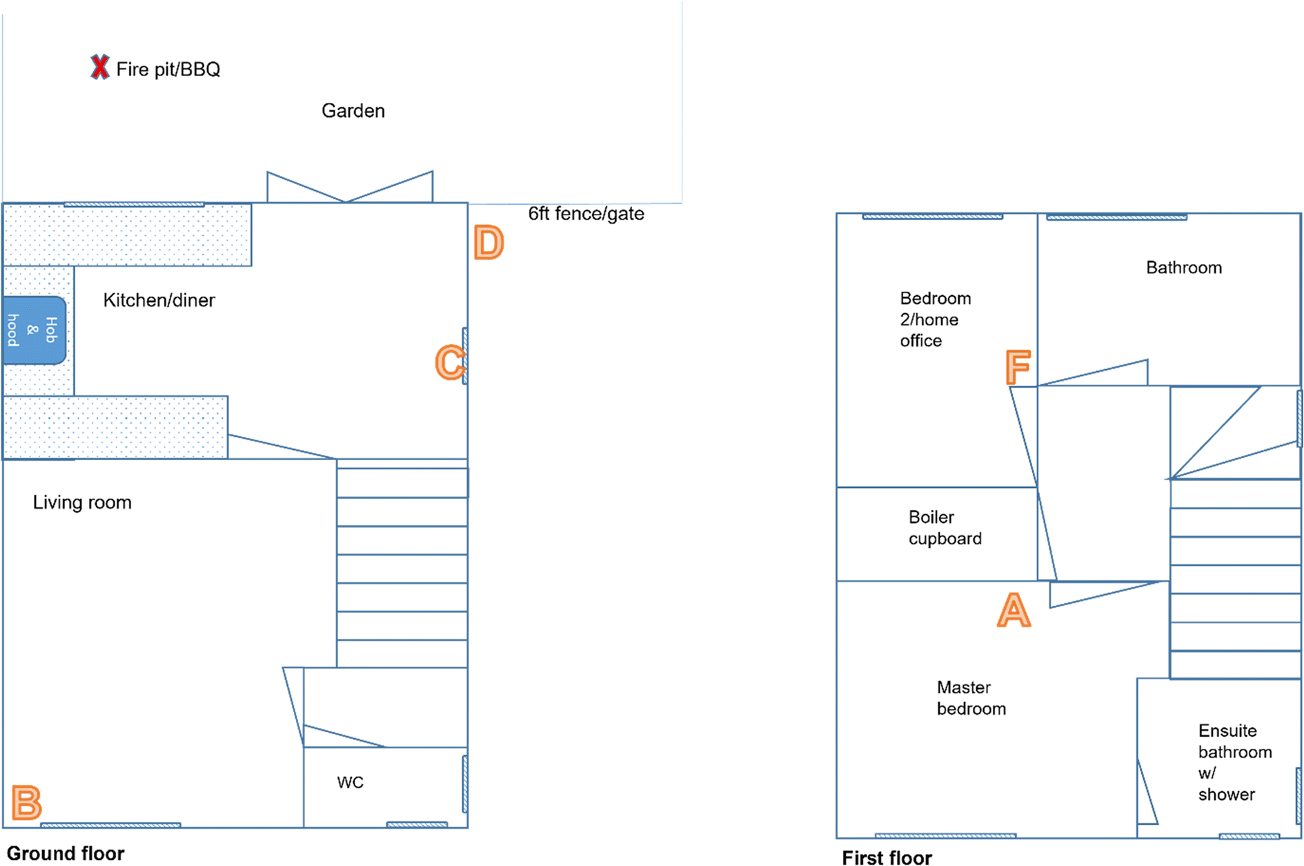Fig. 1 Floor plan of house showing approximate sensor locations with sensor code associated with colocation period.

Table 2 Description of the sensor location by room and description of potential sources and ventilation by room. NB. Sensor E was earmarked to be deployed in the ensuite bathroom however it had an issue with the Arduino board in between colocation study and data collection so was unable to be deployed for this study

Room	Sensor ID	Potential particulate sources of particulates	Ventilation	Sampling location details
Master bedroom	A	Vacuuming, cleaning, ensuite shower/bathroom, aerosol cosmetics/toiletries	Windows, ensuite extractor	On top of chest of drawers, near where aerosols are kept. Inlet and exhaust are facing into the room
Living room	B	Candles, oil burner, cleaning, vacuuming	Window	On top of small cabinet. Inlet and exhaust facing into room
Kitchen/diner	C	Cooking (frying/boiling/oven), cleaning, vacuuming	Windows, double external door, extractor fan	On windowsill, opposite side of room from hob and extractor, above dining table. Inlet and exhaust facing into the room
Outside	D	Traffic, nearby agricultural emissions, domestic burning, bbqs, ambient concentration	N/A	Attached to post on edge of property, near to double doors of kitchen. Farm facing side of property
Bedroom 2/home office	F	Drying laundry	Window	On shelf located against wall in middle of room. Inlet and exhaust are facing into the room

---

All indoor sensors were kept between 1–1.5 m height as furniture/fixings allow whilst the exterior sensor was mounted at ∼2 m. Table 2 outlines the key characteristic of each room the sensors were deployed in.

The sensors used are described in detail in Cowell et al. (2022)⁷¹ but are briefly covered here. The PMS5003 were connected to a custom PCB with an Arduino MKRFox1200 and SHT21 for Sigfox connectivity and temperature/humidity measurements respectively, creating a custom sensor platform called AltasensePM. The PMS5003 is a nephelometer which converts light from a laser scattered by particles into a voltage pulse and then a particle count using an undisclosed algorithm.⁶⁷

The PMS5003 is stated by manufacturer to detect particles of diameter >0.5 μm (98% counting efficiency), with a minimum distinguishable particle diameter of 0.3 μm (although at a lower counting efficiency of 50%)⁷⁵ however Ouimette et al., 2022 (ref. 76) reported the PMS5003 detecting particles smaller than this diameter. It has an uncertainty of ±10 μg m⁻³ and ±10% for ranges 0–100 μg m⁻³ and 100–500 μg m⁻³ respectively.

For the indoor units, the PMS5003 was not placed in an enclosure-the electronic housing protected the PCB and batteries only with the PMS5003 unit resting on top to sample. The outdoor unit housed the PCB, batteries and PMS5003 for weather protection-the enclosure was suspended from a post with the PMS5003 inlet and exhaust located at the base of the enclosure.

The SHT21 has a small cap cover made of a protective mesh to stop the accumulation of condensation on the sensor. Altasense devices are identified and differentiated by letter-with 5 devices labelled A, B, C, D and F throughout the colocation analysis, before being assigned to a room (a 6th sensor, labelled E suffered microcontroller failure so was removed from the study). The Altasense devices record data every 15 minutes. The unit runs for 1 minute to stabilise before taking a reading, takes an instantaneous measurement at the end of the minute and then powers down for the rest of the 15 minutes period. This sampling method enables maximum power efficiency to extend battery life. Data capture is also limited to every 15 minutes by the allowance of message transmission on the Sigfox network. This compromise of frequency allows for deployment of 8–10 weeks+.

3.2 Activity log

A manual electronic log of activity that could potentially generate particulates or alter ventilation was created for indoor and outdoor environments at the study outset. For indoor rooms, key activities included but were not limited to cooking; cleaning; burning of candles; vacuuming; opening windows and oven extractors. As the dwelling main bedroom has an attached ensuite bathroom with shower, the shower usage, bathroom extractor and bathroom cleaning times were also noted. The outside activity noted was only activity from the garden of the study property-including fires and BBQs. Although there were other outdoor influences such as vehicular traffic in the village, emissions from the nearby farm and neighbours domestic burning, these could not be captured in a consistent way as start and end times were not known. Definitions/descriptions of the activity recorded are outlined in Table 3.

Table 3 Definitions of the various activities recorded in the activity log

Activity	Description/definition
Cooking-oven	The electric oven is in use on a standard oven/baking setting (not grilling)
Cooking-frying	Frying or using a pan to cook without water on the gas stove
Cooking-boiling	Boiling/steaming food using a pan and water on the gas stove
Cooking-other	Use of a grill/toaster or other method of cooking not described above
Extractor	In the kitchen this refers to the stove top extractor which is manually controlled
	In the bathroom/bedroom this refers to the room extractor which is manually controlled
Cleaning	Cleaning of surfaces-including dusting, use of antibacterial products and wiping down work areas. Excludes dishwasher, washing machine or washing dishes
Vacuuming	Use of a vacuum cleaner to clear floor. A SHARK bag less vacuum cleaner is used in this household
Window/external ventilation	The opening of a window or in the case of the kitchen external window or door or both opened (external ventilation)
Candle	Lighting of a candle within the room
Fire	Outdoors only-a small firepit burning wood is lit
BBQ	Outdoors only-a coal powered BBQ is in use
Oil burner	An oil burner which uses a tea light candle to melt scented wax melts into an oil is being used
Shower	Ensuite bathroom shower is in use

---

3.3 Colocation and correction of low-cost sensors

Literature suggests that low-cost particulate sensors should be calibrated in an environment similar to which they will be sampling in, due to particulate composition affecting performance.^69,77 Whilst traditionally this is against a regulatory grade instrument such as a gravimetric method or gravimetric equivalent such as a FIDAS, the coronavirus restrictions and policies at the time of this work, we were unable to install an instrument of this type within the sampling home. To this end, the AltasensePM devices which sampled indoors were calibrated indoors in the same property by co-locating with a TSI DustTrak II 8532 handheld model, a laboratory grade instrument. Co-location (1 week) took place within the kitchen of the property. Although this may not as rigorous colocation as against a regulation instrument and it may be best to regard sensor concentrations as relative values rather than absolute, this method is well suited and scalable to in-home studies as it was less intrusive on occupants lives due to the small size/reduced noise of the instrument and required less staffing than a regulatory instrument. This also allows comparison of a low-cost sensor (<£100) against a mid-cost (£4000–7000) laboratory grade instrument.

As this study aims to create a correction factor that encapsulated all of the typical activity within a home, participants were encouraged to proceed with activity as normal – thus ensuring the correction factor captures the majority of typical particulate generating activity that normally occur within the home. Fig. 2 shows activity over the colocation week and the hourly average time series in Fig. 3 shows how the DustTrak and Altasense demonstrate similar patterns in concentrations over time (generated before any data manipulation of the DustTrak data to match the AltasensePM sampling frequency).

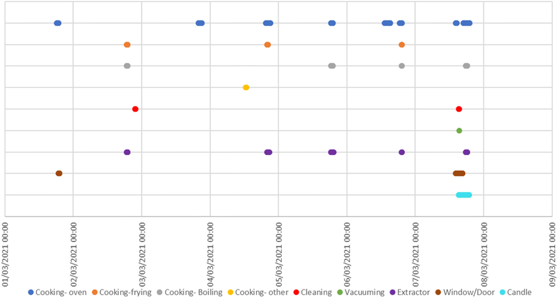Fig. 2 Kitchen activity log for the colocation period. Dots show time when activity was occurring.

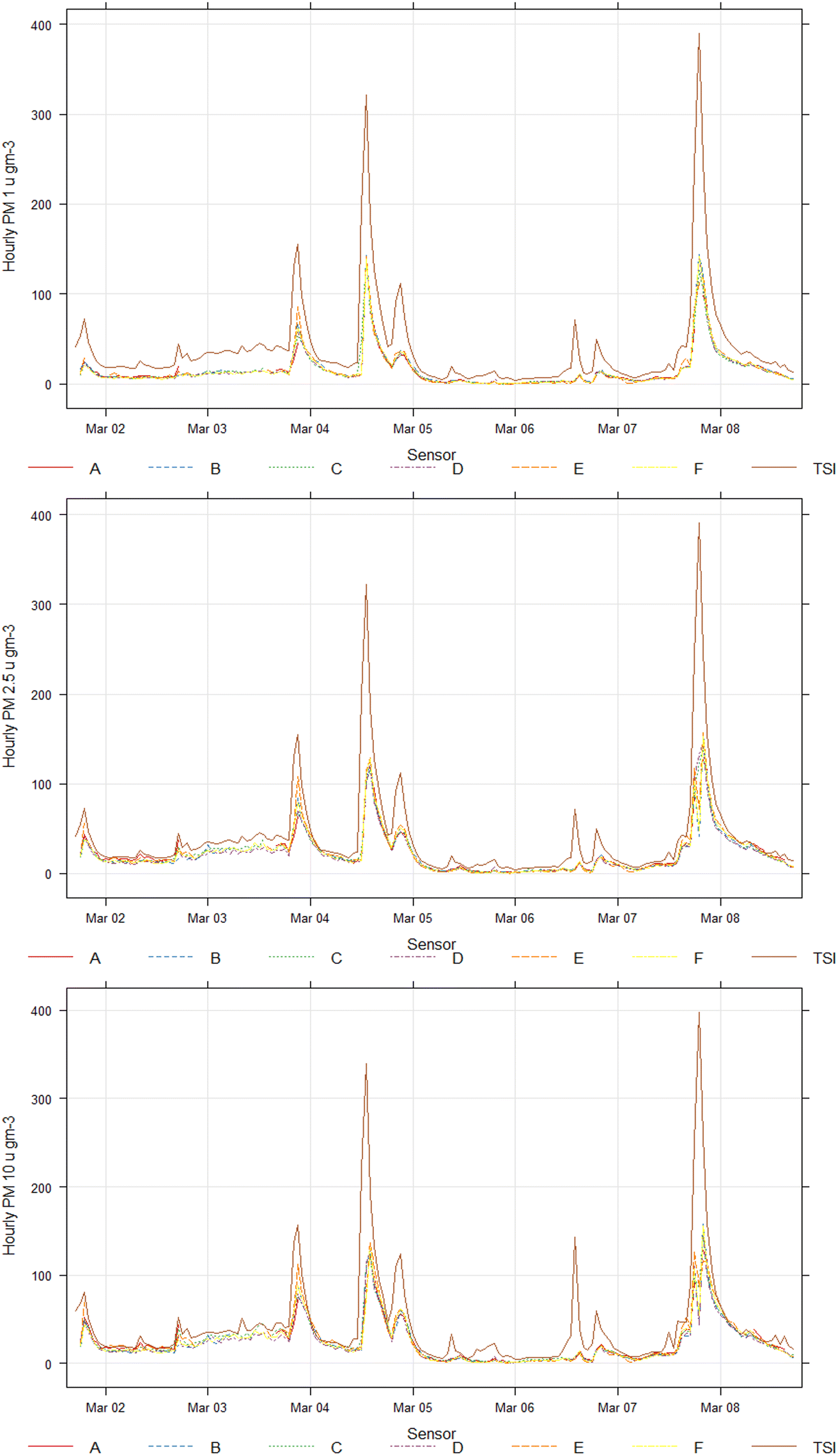Fig. 3 Hourly average time series for AltasensePM devices and TSI for colocation week.

The DustTrak is a light scattering laser photometer with an inbuilt pump designed for monitoring in a range of scenarios, including manufacturing and IAQ.⁷⁸ Although designed for battery powered sampling, this study used mains power to enable continuous measurement for the colocation week as battery life was not able to support this. The DustTrak has a sampling ranging of 1 μg m⁻³ to 150 mg⁻³ and a resolution of ±1% or 1 μg m⁻³ whichever is largest.⁷⁸ This study used a logging frequency of 1 minute. Whilst not a gravimetric or equivalent reference instrument, the DustTrak has been successfully used to draw conclusions about IAQ; including comparing concentration to WHO guidelines and generating I : O ratios within past literature^79,80.Wallace et al., 2011 (ref. 81) report a DustTrak vs. gravimetric r² of 90%, although they also report issues with multiplicative bias. Overall, this suggests the DustTrak should be suitable for calibrating the sensors to generate indicative and relative concentrations.

As the AltasensePM records an instantaneous measurement every 15 minutes, each AltasensePM reading was matched with its time matched counterpart from the DustTrak for data analysis and correction models with the remainder of the DustTrak data discarded.

Table 4 shows key statistics from the colocation period. Absolute values from the PMS5003 consistently under-read compared to the DustTrak – the slope is low (0.28–0.52) between Altasense vs. DustTrak and the DustTrak also recorded maximum values significantly higher than that of the AltasensePM for all species. 181, 197 & 196 μg m⁻³ are the maximum values recorded by the AltasensePM's for PM₁, PM_2.5 and PM₁₀ respectively compared to 507, 508 & 541 μg m⁻³ for the DustTrak. Initially, it may appear that the sampling range is likely to play some part here as the maximum values from the DustTrak are all >500 μg m⁻³ stated as max effective range for the PMS5003, however the AltasensePM do not record any maximums within 300 μg m⁻³ of the stated limit suggesting the Plantower PMS5003 are under-performing well below the stated limits. However, previous literature has shown the PMS5003 can report concentrations much greater than the suggested manufacturer limit.⁸² Alternatively, the variations in maximum values could be an impact of the intermittent sampling method of the AltasensePM-whilst the DustTrak measurements were compared at the same sampling frequency as the AltasensePM recorded, the DustTrak was sampling continuously whilst the AltasensePM powered down between measurements. This could be an indication that the powering up/down of the sensor is limiting the capture of peaking concentrations.

Table 4 Results of AltasensePM colocation with DustTrak

Sensor ID	Species	Pearson's r	R ^2	Max	Min	Mean	Slope
A	PM1	93	0.87	98.0	0	11.3	0.37
	PM2.5	92	0.85	127	0	18.16	0.52
B	PM1	91	0.82	171	0	16.07	0.36
	PM2.5	72	0.52	185	0	21.13	0.32
C	PM1	93	0.87	174	0	15.22	0.34
	PM2.5	79	0.62	185	0	22.3	0.34
D	PM1	88	0.78	171	0	15.15	0.33
	PM2.5	78	0.61	197	0	21.36	0.35
F	PM1	90	0.81	168	0	15.56	0.35
	PM2.5	72	0.52	189	0	23.04	0.32

---

Linear correlation between the reference and low-cost sensors was strong and Pearson's r values between Altasense and TSI DustTrak are 0.84–0.93, 0.72–0.92 and 0.65–0.88 for PM₁, PM_2.5, and PM₁₀ respectively (see Table 4 for full details) for raw data. Fig. 3 also highlights inter-sensor comparability between the AltasensePM devices, demonstrating good intersensory correlation (Pearson's r = 84–99, 87–99, 86–98 and for PM₁, PM_2.5, and PM₁₀ respectively). This suggests the sensors are comparable between themselves and therefore suitable for a network deployment which focuses on difference in concentrations by location.

3.3.1 Indoor sensor correction. Data used for the indoor correction was collected ahead of deploying, during 01.03.21–07.03.21 and the colocation data from 8th March was used to check the success of a correction method. It is clear from Fig. 3 that the correction for the AltasensePM needs to address the discrepancy experienced during peaks of particulate concentrations. Before correcting data, all corresponding AltasensePM values where DustTrak concentrations exceeded 500 μg m⁻³ were removed as these values are beyond the manufacturer stated limits of measurement for the Plantower PMS5003. This is to follow manufacturer guidelines for use of the Plantower, but does suggest a threshold-step change, rather than a gradual trend, in performance of a sensor. Whilst this may be the case, the decrease in performance could be due to increasing undercounting at higher concentrations from coincident particles which would be more likely to present a gradual trend in performance decline. When plotting DustTrak : AltasensePM by AltasensePM, it becomes clear that there is a logarithmic pattern (Fig. 4). DustTrak : AltasensePM ratio drops when the Altasense reports ∼20 μg m⁻³ and thus under-reading occurs most as AltasensePM recorded concentrations increase. This is likely due to the PMS5003 atmospheric correction factor, an undisclosed algorithm Plantower recommend for ambient monitoring that reportedly reduces concentrations >30 μg m⁻³.⁸³ Whilst ideally an IAQ study would utilise the standard particle correction setting on the PMS5003, the AltasensePM was initially designed for use in an ambient monitoring network and this study was a result of lockdown delays to ambient sampling.

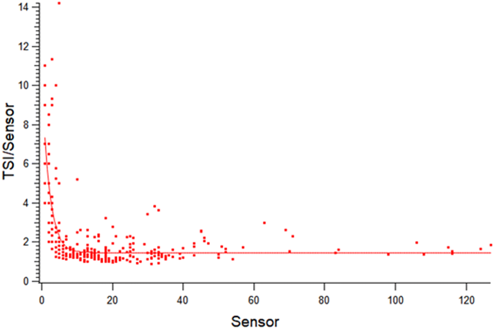Fig. 4 TSI : Altasense ratio by sensor concentration demonstrations a logarithmic relationship between the 2 device types where the AltasensePM under-estimates concentrations.

A range of correction models (scaling factors) were explored: linear correction models failed to allow for the concentration-dependent variation in performance between reference and low-cost sensors didn't address the discrepancy in peaks. Polynomial models were plotted for reference: AltasensePM and a quadratic model proved good fit. Fig. 5 shows results of a colocation after correction by an individual quadratic model for each sensor.

Fig. 5 Hourly average data from a colocation with TSI post sensor correction (“cor”) by polynomial model.

3.3.2 Ambient sensor correction. Evidence suggests that for ambient monitoring, the effect of humidity on low cost sensors based on light scattering techniques calls for further correction past calibration.^69,84 A previous study has demonstrated that the PMS5003 used in the AltasensePM requires a multi-linear model for correcting data when calibrating against a reference grade nephelometer (PALAS FIDAS).⁷¹ Whilst the indoor measurements are unlikely to reach >85% humidity the outdoor sensor likely will, thus in these instances the multi-linear correction developed in Cowell et al., 2022 (ref. 71) will be applied. To achieve this, sensor D (used outside) was back calibrated. After being deployed as part of this study, sensor D (used outside) was taken to Birmingham Air Quality Supersite (BAQS) and collocated with a PALAS FIDAS to generate data for a multi-linear correction based on humidity.

3.4 Data validation

There is a need to validate low-cost sensor data-even after correction as sensors may malfunction and misreport data following deployment. This is particularly important when data cannot be checked against a nearby reference instrument. Lu et al., 2021 (ref. 85) & Mousavi and Wu, 2021 (ref. 23) suggest a data validation method for quality control. The data validation steps outlined below are based upon those used for the commercial PurpleAir network, the devices of which utilise the same Plantower PMS5003 sensors as AltasensePM in both an indoor and outdoor setting.^23,85 Data validations are adapted from these methods (minus steps which utilise the dual reading channels from having 2× PMS5003 within each PurpleAir unit as this is not applicable to the AltasensePM). Validation steps are outlined below:

(1) Discard data of concentration >500 μg m⁻³ as this is outside of the manufacturers stated limitations of the sensor. Only 1 value fell beyond this threshold-a reading from the kitchen for PM₁.

(2) A completeness criterion-only use sensors with >75% completeness of data. Results from presence are show in Table 6.

3.5 Novel development in understanding of the Plantower PMS5003 for coarse size fractions

Since the original design of the AltasensePM, research has highlighted challenges surrounding the measurement of PM₁₀ by low cost nephelometers. Hagan and Cross, 2022 (ref. 86) highlight multiple studies that indicate the inability of some such sensors to reliably report coarse PM fractions (>PM_2.5).^76,87,88 They suggest that, in instances where PM₁₀ seems to be reporting in agreement with a reference, that it is likely there are minimal larger particles present and the sensor is effectively reporting smaller size fraction concentrations that happen to correlate with PM₁₀ concentrations. Ouimette et al., 2022 (ref. 76) attribute the lower retrieval of PM₁₀ to laser geometry and particle losses before reaching the laser (path of PM sample is too narrow/tight bends for PM₁₀ to navigate without losses, through inertia) and the inability of the sensor to detect all of the light scattered by larger particles. This is reflected in the colocation week data in this study where PM₁₀ performed worse than the smaller size fractions against a reference instrument (see Table 4). Whilst our calibration efforts improved agreement (Table 5), PM₁₀ was still had the weaker relationship with the reference instrument than PM_2.5. PM₁₀ is reported in figures throughout this study to avoid censorship of data and to provide insight into sensor performance. However, authors are aware that reported PM₁₀ are likely to be more reflective of smaller particle sizes than PM₁₀ itself, and thus do not focus on PM₁₀ during discussion and urge readers to be cautious in drawing conclusions from PM₁₀ concentrations.

Table 5 r ² values of AltasensePM and DustTrak from colocation period after correction of sensors with a quadratic model. NB. Sensor A had significantly less data points (n = 14, rather than n = 71 for other units) throughout the post correction co-location than other sensors due to a power loss, it's poor performance may be linked to this

	PM1		PM2.5
	Slope	r ^2	Slope	r ^2
A	2	0.73	2.4	0.79
B	0.93	0.82	1.4	0.88
C	0.9	0.81	1.3	0.89
D	0.8	0.78	1.3	0.92
F	0.79	0.7	1.5	0.85

---

Table 6 Presence of sensors within study period. All are above the 75% completeness required as part of the data validation steps

Location	Bedroom	Living room	Kitchen	Outside	Office
Presence (%)	98.4	86.5	93.6	83.3	98.5

---

Another important feature to note from the literature is debate around the ability of low-cost sensors to report multiple size fractions. Ouimette et al., 2022 (ref. 76) and Kuula et al., 2020 (ref. 87) report that the PMS5003 is most effective at recording PM₁ concentrations and Kuula et al., 2020 (ref. 87) report that it may not accurately distinguish between size fractions well, particularly in unstable ambient air size distributions. Unlike ambient air, there are not large regional events that will drastically change the composition/size distribution of particulates from the from those experienced as part of the calibration and Kuula et al., 2020 (ref. 87) also suggest that with stability, the PMS5003 can be calibrated to report PM_2.5 relatively well. Therefore, whilst PM₁ is reported in this study, authors also felt it was important to report PM_2.5 as this allows for comparison to global guidelines for PM.

3.6 Data analysis

Data analysis explores first the sensor presence presented in Section 3.4 as this can provide key insight into the success and pitfalls of sensor performance.

Indoor : outdoor (i : o) ratios were calculated from hourly averaged data for each room to allow for data matching. An average indoor concentration hourly time series was also generated from the mean concentrations of all indoor measurements so an average indoor : outdoor ratio could also be analysed.

Activity log data was transformed into a time series so that activities could be plotted and analysed against concentration time series.

Data analysis made use of the OpenAir package in the R programming tool.^89,90

4 Results & discussion

4.1 Particulate concentrations and activity

Fig. 6 and Table 7 present the corrected concentrations experienced within the property for the study period. Assuming the short duration measurements reported here were typical of those present over longer time periods (i.e., annually), of the 5 rooms, PM levels in all 4 rooms exceeded both the WHO 2021 and 2005 annual ambient particulate concentration guidelines of 10 μg m⁻³ (2005) and 5 μg m⁻³ (2021) for PM_2.5,⁵ if extrapolated to annual levels. Ambient PM_2.5 was lower, not exceeding the 2005 guidelines and reporting just above the 2021 guideline concentration.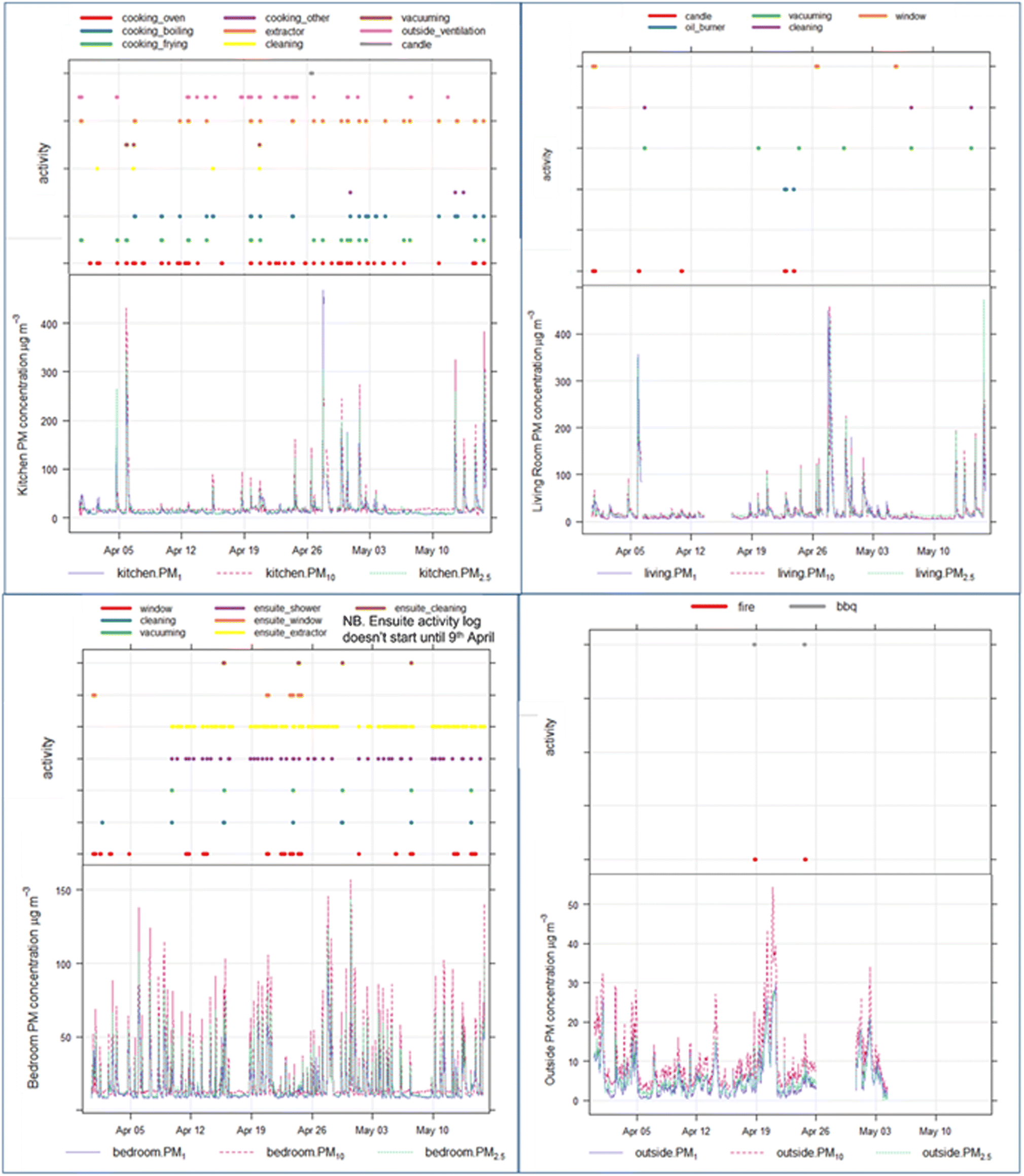

Fig. 6 Hourly average PM concentrations by room with activity log for each room above. Note kitchen and living room are located next to each other and share a doorway which was often open. Activities may also be affecting concentrations in other rooms.

Table 7 Indoor : outdoor ratio for period of the study by room calculated from hourly average concentration values and mean concentrations for the whole study period. Mean is colour coded to represent concentrations above and below WHO guidelines for PM_2.5 and PM₁₀. Green = mean concentration less than WHO 2021 Annual guideline. Orange = mean concentration falls inbetween WHO 2021 and WHO 2005 guidelines. Red = mean concentration greater than WHO 2005 annual guideline

---

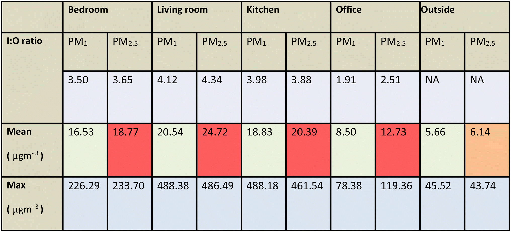
This suggests that if the 7 weeks of study were reflective of a typical year in the property, the bedroom, kitchen and living room could be considered as exposure that is harmful to health by WHO guideline levels. Maximum concentrations recorded significantly exceed WHO guidelines-the living room reported highest concentrations (488, 486 & 481 μg m⁻³ for PM₁, PM_2.5, and PM₁₀ respectively) followed closely by the kitchen (488, 462 & 478 μg m⁻³ for PM₁, PM_2.5, and PM₁₀ respectively). Outside reported the lowest peak concentrations followed by the home office.

Cooking and ventilation (both external via windows and mechanical via extractor fans) proved easier to analyse within this study as these activities all took place over periods time greater than the AltasensePM sampling resolution, whereas activity such as cleaning (spraying of cleaning sprays) and vacuuming occurred in short bursts which may not have been coincident with a sensor measurement. This highlights a notable disadvantage of the low power approach used by the AltasensePM to conserve battery power where readings are only taking for 1 minute of every 15-sensors can capture PM variability over the period of 15 minutes to hours but cannot capture variability that occurs in short bursts.

The following analysis of activity vs. concentrations focuses on cooking and ventilation due to this.

4.1.1 Cooking and downstairs concentrations. Cooking by oven was the most common type of cooking, with 75.5% of all cooking recorded being via oven. “Other” (defined in Table 3) was the least common type of cooking. The extractor was used 81% of the time when cooking was occurring and external ventilation via an open window or external door was used 44% of the time cooking occurred.

In the living room, maximum PM levels did not coincide with any recorded activity in that room but PM₁ and PM_2.5 did directly coincide with cooking with the oven in the kitchen. Whilst other max recordings in the kitchen and living room do not directly match with cooking being recorded at that time, the max PM₁ and PM_2.5 recording in the kitchen also occurred between 18:00 and 19:30 which is during the window that cooking regularly occurred on a daily basis (Fig. 7). Although the measurements didn't directly coincide, this is most likely due to the 15 minutes sampling time of the sensor occurring just outside of the time cooking was occurring. This highlights a compromise of maintaining the battery power and IoT communications by reducing sampling frequency and thus not capturing cooking events at as high resolution as other studies. From the diurnal plot of PM_2.5 concentrations, PM levels in the kitchen and living room appear to be correlated particularly in the evening peaks around meal preparation time and this is reflected in the hourly average correlation with Pearson's r values of 93, 88 and 83 for PM₁, PM_2.5 and PM₁₀ respectively. The higher correlation occurring with PM₁ between the 2 rooms suggests that the smaller particles are more effective at travelling between rooms-this is expected as larger particles are likely to settle sooner due to weight or be filtered out during transmission by walls/doors.³⁰ Whilst PM levels in the rooms correlate around the peaks, they differ in their decline rate after cooking occurs with the kitchen returning to a lower concentration baseline much quicker than the living room does, with the living room still experiencing elevated peaks in concentrations into the early morning hours. This could be attributed to (a) lack of an extraction fan in the living room (unlike the kitchen) to reduce concentrations or (b) other sources in the living room generating further PM in the evening (candle/oil burner although not as frequent a source as cooking, was used in the evening a few times). Fig. 8 demonstrates the extreme values recorded during various activities with cooking by oven and frying coinciding with extreme high readings, however oil burning and candles do not produce peaks >200 μg m⁻³ and it appears the extreme peaks are associated with cooking in the adjacent kitchen. Extractor fans have been demonstrated by literature to reduce PM concentrations during and after cooking.⁹¹ A similar phenomena was also recorded in Kim et al., 2018 (ref. 55) where living room concentrations were greater than kitchen concentrations after a cooking event when extractor fans are in use in the kitchen alone. This highlights the importance of considering dispersion of particles from a cooking event, and ventilation in adjacent rooms, not just a kitchen.

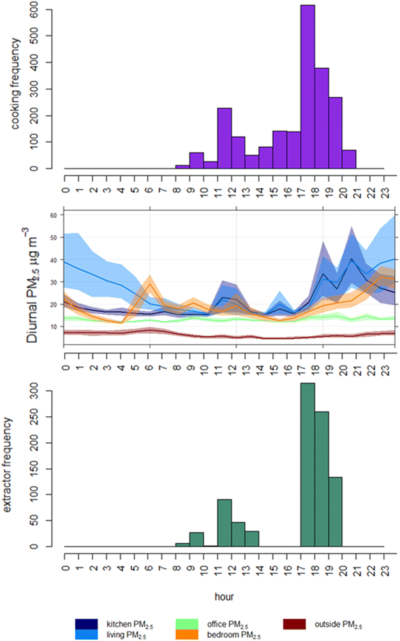Fig. 7 Histograms demonstrating the frequent times of day for cooking activity (all cooking types combined) and kitchen extractor fan usage alongside diurnal patterns of PM_2.5 concentrations by room. NB. Frequency here describes the number of minutes the activity was marked as “present” and is separated into bins by hour of day.

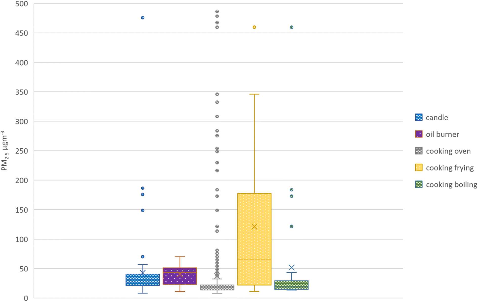Fig. 8 Distribution of PM_2.5 concentrations in living room during various activities. Cooking occurred in the adjoining kitchen whilst oil burner and candle were located within the living room itself.

4.1.2 External ventilation. Windows or external doors were open for 10 805 minutes or 180.08 hours across the property for the 7 week period (bedroom window 5770 minutes, ensuite window 1652 minutes, living room 645 minutes, kitchen 2738 minutes). Sensors captured particulates data for 602 minutes where the window was open in the room they were directly measuring in (175 minutes in kitchen, 385 minutes in bedroom (bedroom window only), 42 minutes in living room). As this study occurred in spring, this amount is likely to increase in the summer months and reduce in the winter due to seasonal ambient temperature changes. Whilst the bedroom window opening occurred quite evenly spread across the day (with windows closed at night), the kitchen windows are most frequently opened between 4–6 pm (median hour of window opening 5 pm) coinciding with cooking activity frequency (Fig. 7). Fig. 10 demonstrates the excess in extreme high values recorded when windows are closed vs. when windows are open across all rooms for PM₁ and PM_2.5. It is difficult to draw conclusions regarding the influence on external ventilation via windows/doors for the kitchen as PM levels were also being driven by other activity-notably cooking described above. The mean in the kitchen was higher with windows open, this may be due to the coinciding with cooking activity times, yet opening windows appears to reduce exposure to extreme values with less extreme high values recorded when windows or external door is open. A Mann–Whitney U test reported a statistically significant difference between kitchen PM concentrations when windows are closed vs. open (for PM₁ and PM_2.5, p = 2.2 × 10⁻¹⁶) with a 95% confidence that median difference will be between 8.6 to 4.9 μg m⁻³ and 7.7–5.4 μg m⁻³ for PM₁ and PM_2.5 respectively.

As the bedroom has less activity recorded than the kitchen and has window openings more evenly spread across the day, there is less of a connected impact to another activity and thus differences may prove more insightful in terms of the impact of windows opening. Bedroom concentrations are statistically different when windows are shut vs. open in the bedroom itself (p = 0.0031 and p = 0.0022 for PM₁ and PM_2.5 respectively), with a 95% confidence of a 2.7–7.3 μg m⁻³ difference between having windows closed and open. Median and mean values for windows shut/open are close in value (18.9 μg m⁻³, 17.2 μg m⁻³ means and 19.5 μg m⁻³, 18.6 μg m⁻³ medians for PM_2.5) suggesting the major difference is in the reduction of high outlier values when windows are open.

In the context of this property (suburban, relatively low ambient PM concentrations) it is likely that the opening of windows is reducing the extreme highs generated from indoor sources, but an impact on mean concentrations is more uncertain. This may be due to the impact of other activity influencing concentrations at the same time as the windows being open (cooking), although literature suggests reductions in mean PM_2.5 from window ventilation alone may be possible.^92,93 However, in other settings with poor ambient concentrations window ventilation is unlikely to be effective at reducing PM concentrations as it increases the infiltration of ambient air and hence potentially elevated PM concentrations into the home.

4.2 Indoor : outdoor ratios

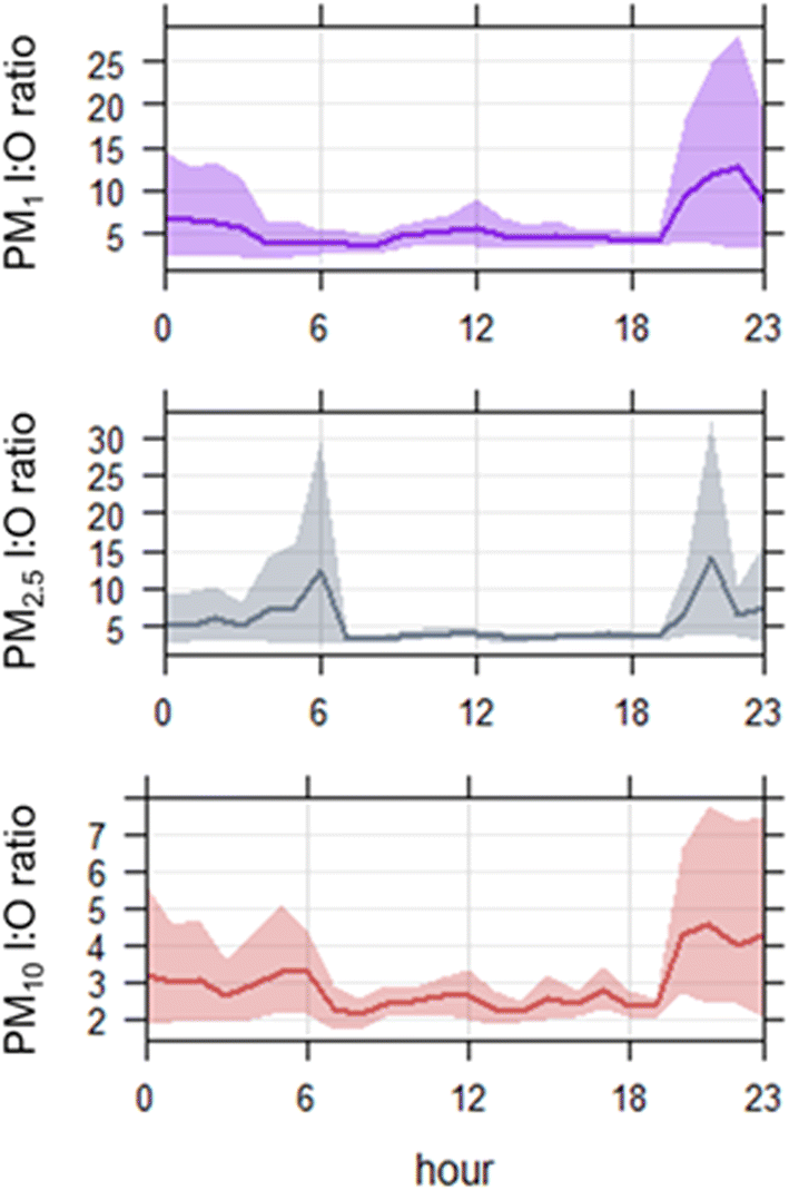
Indoor particulate concentrations were generally higher than ambient-the average I : O ratio for the property was 5.8 and 5.5 for PM₁ and PM_2.5 respectively and the I : O ratio by room is outlined in Table 7. The PM_2.5 ratio is higher than ratios found in Kang and Choi, 2020 (ref. 94) literature review of I : O ratios where I : O PM_2.5 is generally reported <2.0. This could be due to the relatively low ambient PM_2.5 and PM₁ (mean concentration 6.14 μg m⁻³ and 5.66 μg m⁻³ respectively). The living room experienced the highest I : O ratio, followed by the kitchen, then bedroom with the office having the lowest ratio. Fig. 9 demonstrates the diurnal pattern of I : O ratio-whilst all PM size fractions experienced peaks in the evening time only PM_2.5 experienced peaks in the morning with ∼6 am coinciding with showering and cosmetic aerosol use. As diurnal ambient PM concentrations are fairly stable and doesn't fluctuate alongside the indoor concentrations (Fig. 7) and I : O ratio increases during peak activity time, this suggests that the major sources of indoor PM come from within the property itself rather from dispersion of ambient PM into the home.

Fig. 9 Diurnal patterns of average I : O ratio by PM size fraction (average concentration of all inside locations: outside concentration).

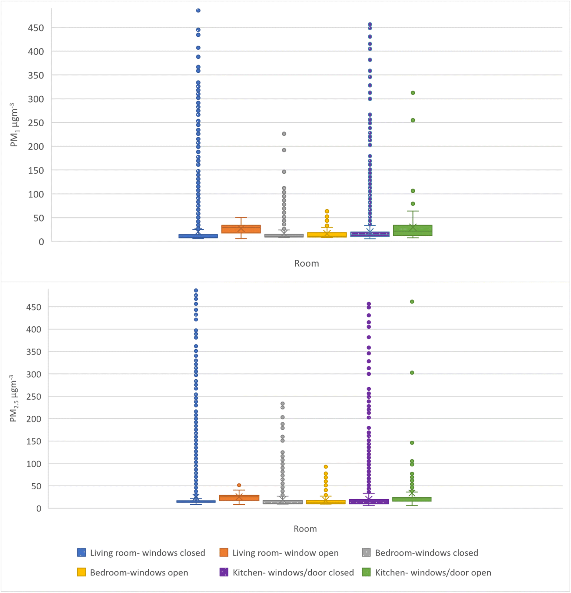Fig. 10 Boxplot of PM₁ and PM_2.5 concentrations by room for when external windows/doors are open vs. when they are closed. NB. Bedroom only refers to bedroom window, not ensuite bathroom window.

4.3 Limitations

Whilst this study presents meaningful insight into the application of low-cost, IoT sensing networks for measuring indicative particulate concentrations, there are some factors that limit the output of the study.

The pandemic and lockdown restrictions in place at the time of data collection may have limited residents' behaviour-generally spending more time inside, potentially eating out less and thus cooking more etc. Whilst this highlights the need for understanding of IAQ, it also means that this may not be reflective of ‘normal’ behaviour as we transition into a post-Covid context. This could also impact the generation of a generic correction factor for a home, as the particulate generating activities may have been influenced by the change in behaviour. Thus, the correction factor may not be reflective of pre or post-pandemic behaviour, although the method to develop a new correction factor should still be valid allowing for updates with behaviour change.

This study is a short term data collection which may not be directly reflective of the data used to generate longer term guidelines.⁵ However, since this study's data collection occurred, the platform which hosts the AltasensePM devices has been developed to apply correction models to data in near-real time which would reduce manual workload of correcting data and enhance sensors ability to generate easy-to-use long term time series.

5 Conclusions

This study started with 2 key criteria:

(1) Validate the application of IoT low-cost sensor networks for indoor air quality including the development of a method for correcting and validating low-cost data within an indoor setting.

(2) Evaluate the impact of human activity and different sources on PM levels throughout a residential property, inclusive of indoor : outdoor ratios.

Sensor validation is described in the methods section, where with correction and data validation steps AltasensePM was able to detect with good accuracy (r² > 0.7 for PM₁ and >0.79 for PM_2.5) particulate concentrations. Importantly, sensors had really strong inter-sensor correlation (Pearson's r > 84 for all size fractions) meaning that as a network deployment they were suitable for comparing differences between locations. The IoT enabled sensors had good presence (83–99%) and were able to detect diurnal patterns within data. Their major drawback was time resolution, which was compromised by battery life to enable sensors to be mobile and unintrusive to deploy. Whilst peaks were captured, AltasensePM was unable to capture high resolution detail and some shorter activity periods were harder to assess as the sensor wasn't always recording as they occurred. Overall, the low cost IoT network provided valuable insight into relative particulate concentrations and could be adjusted to be mains powered to increase measurement frequency considering that power access is rarely an issue in many households.

Indicative indoor concentrations exceeded WHO guidelines for particulates and were higher than ambient concentrations. Cooking was clearly detected to influence particulate concentrations and often lead to extreme peaks in concentrations. Cooking by oven and frying increased particulate concentrations in both the kitchen and living room area despite the use of an extractor fan and windows over cooking periods. The living room experienced higher concentrations than the kitchen-this may be due to a lack of extractor fan in the living room and the lower use of windows for ventilation compared to the kitchen. The use of window opening for increased ventilation clearly reduces extreme peaks in concentrations and thus could be an affordable and effective suggestion to residents to reduce exposure to short term high concentrations, depending on location and ambient conditions.

Author contributions

Conceptualization NC, LC and WB. Methodology NC, LC, WB, DS. Software NC, DS. Validation NC, LC, WB. Formal analysis NC. Investigation NC. Resources LC, WB, NC. Data curation NC. Writing – Original draft NC, LC, WB. Writing – review & editing – SB, AS, DS. Visualization NC, DS. Supervision LC, WB. Project administration NC. Funding acquisition WJB, LC.

Conflicts of interest

There are no conflicts to declare.

Acknowledgements

The authors would like to thank the residents of the study property for their participation in the project. The assistance of Dr Siqi Hou and colleagues at the Birmingham Air Quality Supersite at the University of Birmingham in the colocation of sensors as part of this project is also acknowledged.

References

1. J. González-Martín, N. J. R. Kraakman, C. Pérez, R. Lebrero and R. Muñoz, A state-of-the-art review on indoor air pollution and strategies for indoor air pollution control, Chemosphere, 2021, 262, 128376.
2. World Health Organisation, Air Pollution: Impacts Online, 2022, available from: https://www.who.int/health-topics/air-pollution#tab=tab_2.
3. G. Guyot, M. H. Sherman and I. S. Walker, Smart ventilation energy and indoor air quality performance in residential buildings: A review, Energy Build., 2018, 165, 416–430.
4. S. Domínguez-Amarillo, J. Fernández-Agüera, S. Cesteros-García and R. A. González-Lezcano, Bad Air Can Also Kill: Residential Indoor Air Quality and Pollutant Exposure Risk during the COVID-19 Crisis, Int. J. Environ. Res. Public Health, 2020, 17(19), 7183.
5. World Health Organisation, WHO Global Air Quality Guidelines. Particulate Matter (PM_2.5 and PM₁₀), Ozone, Nitrogen Dioxide, Sulfur Dioxide and Carbon Monoxide, Geneva, 2021.
6. S. Hegde, K. T. Min, J. Moore, P. Lundrigan, N. Patwari and S. Collingwood, et al., Indoor Household Particulate Matter Measurements Using a Network of Low-cost Sensors, Aerosol Air Qual. Res., 2020, 20(2), 381–394.
7. E. G. Snyder, T. H. Watkins, P. A. Solomon, E. D. Thoma, R. W. Williams and G. S. Hagler, et al., The changing paradigm of air pollution monitoring, Environ. Sci. Technol., 2013, 47(20), 11369–11377.
8. M. Kaliszewski, M. Włodarski, J. Młyńczak and K. Kopczyński, Comparison of Low-Cost Particulate Matter Sensors for Indoor Air Monitoring during COVID-19 Lockdown, Sensors, 2020, 20(24), 7290.
9. E. Ezani, P. Brimblecombe, Z. Hanan Ashaari, A. A. Fazil, S. N. Syed Ismail and Z. T. Ahmad Ramly, et al., Indoor and Outdoor Exposure to PM2.5 during COVID-19 Lockdown in Suburban Malaysia, Aerosol Air Qual. Res., 2020, 20, 200476.
10. A. Susz, P. Pratte and C. Goujon-Ginglinger, Real-time Monitoring of Suspended Particulate Matter in Indoor Air: Validation and Application of a Light-scattering Sensor, Aerosol Air Qual. Res., 2020, 20(11), 2384–2395.
11. J. Zhao, W. Birmili, B. Wehner, A. Daniels, K. Weinhold and L. Wang, et al., Particle Mass Concentrations and Number Size Distributions in 40 Homes in Germany: Indoor-to-Outdoor Relationships, Diurnal and Seasonal Variation, Aerosol Air Qual. Res., 2020, 576–589.
12. R. Xu, X. Qi, G. Dai, H. Lin, P. Zhai and C. Zhu, et al., A Comparison Study of Indoor and Outdoor Air Quality in Nanjing, China, Aerosol Air Qual. Res., 2020, 20(10), 2128–2141.
13. B. C. Singer and W. W. Delp, Response of consumer and research grade indoor air quality monitors to residential sources of fine particles, Indoor Air, 2018, 28(4), 624–639.
14. Z. Wang, L. Calderón, A. P. Patton, M. Sorensen Allacci, J. Senick and R. Wener, et al., Comparison of real-time instruments and gravimetric method when measuring particulate matter in a residential building, J. Air Waste Manage. Assoc., 2016, 66(11), 1109–1120.
15. Y. Jeon, C. Cho, J. Seo, K. Kwon, H. Park and S. Oh, et al., IoT-based occupancy detection system in indoor residential environments, Build Environ., 2018, 132, 181–204.
16. W. R. Ott and H. C. Siegmann, Using multiple continuous fine particle monitors to characterize tobacco, incense, candle, cooking, wood burning, and vehicular sources in indoor, outdoor, and in-transit settings, Atmos. Environ., 2006, 40(5), 821–843.
17. M.-P. Wan, C.-L. Wu, G.-N. Sze To, T.-C. Chan and C. Y. H. Chao, Ultrafine particles, and PM2.5 generated from cooking in homes, Atmos. Environ., 2011, 45(34), 6141–6148.
18. H. Chen, R. Du, W. Ren, S. Zhang, P. Du and Y. Zhang, The Microbial Activity in PM2.5 in Indoor Air: As an Index of Air Quality Level, Aerosol Air Qual. Res., 2021, 21(2), 200101.
19. C.-H. Jeong, S. Salehi, J. Wu, M. L. North, J. S. Kim and C.-W. Chow, et al., Indoor measurements of air pollutants in residential houses in urban and suburban areas: Indoor versus ambient concentrations, Sci. Total Environ., 2019, 693, 133446.
20. S. Vilčeková, I. Z. Apostoloski, Ľ. Mečiarová, E. K. Burdová and J. Kiseľák, Investigation of Indoor Air Quality in Houses of Macedonia, Int. J. Environ. Res. Public Health, 2017, 14(1), 37.
21. G. De Gennaro, P. R. Dambruoso, A. Di Gilio, V. Di Palma, A. Marzocca and M. Tutino, Discontinuous and Continuous Indoor Air Quality Monitoring in Homes with Fireplaces or Wood Stoves as Heating System, Int. J. Environ. Res. Public Health, 2016, 13(1), 78.
22. R. Pitarma, G. Marques and B. R. Ferreira, Monitoring Indoor Air Quality for Enhanced Occupational Health, J. Med. Syst., 2016, 41(2), 23.
23. A. Mousavi and J. Wu, Indoor-Generated PM2.5 During COVID-19 Shutdowns Across California: Application of the PurpleAir Indoor–Outdoor Low-Cost Sensor Network, Environ. Sci. Technol., 2021, 55(9), 5648–5656.
24. S. Kim, S. Park and J. Lee, Evaluation of Performance of Inexpensive Laser Based PM2.5 Sensor Monitors for Typical Indoor and Outdoor Hotspots of South Korea, Appl. Sci., 2019, 9(9), 1947.
25. J. Li, H. Li, Y. Ma, Y. Wang, A. A. Abokifa and C. Lu, et al., Spatiotemporal distribution of indoor particulate matter concentration with a low-cost sensor network, Build Environ., 2018, 127, 138–147.
26. K.-H. Kim, E. Kabir and S. Kabir, A review on the human health impact of airborne particulate matter, Environ. Int., 2015, 74, 136–143.
27. J. O. Anderson, J. G. Thundiyil and A. Stolbach, Clearing the Air: A Review of the Effects of Particulate Matter Air Pollution on Human Health, J. Med. Toxicol., 2012, 8(2), 166–175.
28. World Health Organization, Air Quality Guidelines: Global Update 2005: Particulate Matter, Ozone, Nitrogen Dioxide, and Sulfur Dioxide, World Health Organization, 2006.
29. WHO, WHO Guidelines for Indoor Air Quality: Selected Pollutants, 2010.
30. A. H. Goldstein, W. W. Nazaroff, C. J. Weschler and J. Williams, How Do Indoor Environments Affect Air Pollution Exposure?, Environ. Sci. Technol., 2021, 55(1), 100–108.
31. M. Derbez, B. Berthineau, V. Cochet, C. Pignon, J. Ribéron and G. Wyart, et al., A 3-year follow-up of indoor air quality and comfort in two energy-efficient houses, Build Environ., 2014, 82, 288–299.
32. P. Spiru and P. L. Simona, A review on interactions between energy performance of the buildings, outdoor air pollution and the indoor air quality, Energy Procedia, 2017, 128, 179–186.
33. A. Steinemann, P. Wargocki and B. Rismanchi, Ten questions concerning green buildings and indoor air quality, Build Environ., 2017, 112, 351–358.
34. E. D. Vicente, A. M. Vicente, M. Evtyugina, A. I. Calvo, F. Oduber and C. Blanco Alegre, et al., Impact of vacuum cleaning on indoor air quality, Build Environ., 2020, 180, 107059.
35. H. Shen, W. Hou, Y. Zhu, S. Zheng, S. Ainiwaer and G. Shen, et al., Temporal and spatial variation of PM2.5 in indoor air monitored by low-cost sensors, Sci. Total Environ., 2021, 770, 145304.
36. C. J. Lau, M. Loebel Roson, K. M. Klimchuk, T. Gautam, B. Zhao and R. Zhao, Particulate matter emitted from ultrasonic humidifiers—Chemical composition and implication to indoor air, Indoor Air, 2021, 31(3), 769–782.
37. M. Qi, W. Du, X. Zhu, W. Wang, C. Lu and Y. Chen, et al., Fluctuation in time-resolved PM2.5 from rural households with solid fuel-associated internal emission sources, Environ. Pollut., 2019, 244, 304–313.
38. S. Jodeh, A. R. Hasan, J. Amarah, F. Judeh, R. Salghi and H. Lgaz, et al., Indoor and outdoor air quality analysis for the city of Nablus in Palestine: seasonal trends of PM10, PM5.0, PM2.5, and PM1.0 of residential homes, Air Qual., Atmos. Health, 2018, 11(2), 229–237.
39. N. Canha, J. Lage, J. T. Coutinho, C. Alves and S. M. Almeida, Comparison of indoor air quality during sleep in smokers and non-smokers’ bedrooms: A preliminary study, Environ. Pollut., 2019, 249, 248–256.
40. A. Katsoyiannis and A. Cincinelli, ‘Cocktails and dreams’: the indoor air quality that people are exposed to while sleeping, Curr. Opin. Environ. Sci. Health, 2019, 8, 6–9.
41. N. Canha, C. Teixeira, M. Figueira and C. Correia, How Is Indoor Air Quality during Sleep? A Review of Field Studies, Atmosphere, 2021, 12(1), 110.
42. R. A. Accinelli, O. Llanos, L. M. López, M. I. Pino, Y. A. Bravo and V. Salinas, et al., Adherence to reduced-polluting biomass fuel stoves improves respiratory and sleep symptoms in children, BMC Pediatr., 2014, 14(1), 1–5.
43. P. Strøm-Tejsen, D. Zukowska, P. Wargocki and D. P. Wyon, The effects of bedroom air quality on sleep and next-day performance, Indoor Air, 2016, 26(5), 679–686.
44. K. Ahrberg, M. Dresler, S. Niedermaier, A. Steiger and L. Genzel, The interaction between sleep quality and academic performance, J. Psychiatr. Res., 2012, 46(12), 1618–1622.
45. R. D. Nebes, D. J. Buysse, E. M. Halligan, P. R. Houck and T. H. Monk, Self-reported sleep quality predicts poor cognitive performance in healthy older adults, J. Gerontol. B Psychol. Sci. Soc. Sci., 2009, 64(2), 180–187.
46. J. Andruškienė, G. Varoneckas, A. Martinkėnas and V. Grabauskas, Factors associated with poor sleep and health-related quality of life, Medicina, 2008, 44(3), 240.
47. K. Sigurdson and N. T. A. T. Ayas, The public health and safety consequences of sleep disordersThis paper is one of a selection of papers published in this Special Issue, entitled Young Investigators' Forum, Can. J. Physiol. Pharmacol., 2007, 85(1), 179–183.
48. N. H. Wong and B. Huang, Comparative study of the indoor air quality of naturally ventilated and air-conditioned bedrooms of residential buildings in Singapore, Build Environ., 2004, 39(9), 1115–1123.
49. B. Kozielska, A. Mainka, M. Żak, D. Kaleta and W. Mucha, Indoor air quality in residential buildings in Upper Silesia, Poland, Build Environ., 2020, 177, 106914.
50. S. Nandasena, R. Wickremasinghe, A. Kasturiratne, U. Wimalasiri, M. Tipre and R. Larson, et al., Particulate Matter fractions and kitchen characteristics in Sri Lankan households using solid fuel and LPG, bioRxiv, 2018, 461665.
51. M. Shupler, P. Hystad, A. Birch, Y. L. Chu, M. Jeronimo and D. Miller-Lionberg, et al., Multinational prediction of household and personal exposure to fine particulate matter (PM2.5) in the PURE cohort study, Environ. Int., 2022, 159, 107021.
52. C. A. Campbell, S. E. Bartington, K. E. Woolley, F. D. Pope, G. N. Thomas and A. Singh, et al., Investigating Cooking Activity Patterns and Perceptions of Air Quality Interventions among Women in Urban Rwanda, Int. J. Environ. Res. Public Health, 2021, 18(11), 5984.
53. S. Patel, S. Sankhyan, E. K. Boedicker, P. F. DeCarlo, D. K. Farmer and A. H. Goldstein, et al., Indoor Particulate Matter during HOMEChem: Concentrations, Size Distributions, and Exposures, Environ. Sci. Technol., 2020, 54(12), 7107–7116.
54. An Intervention Study of PM2.5 Concentrations Measured in Domestic Kitchens. 39th Air Infiltration and Ventilation Centre Conference, ed. O'Leary C., Jones B. and Hall I., Antibes Juan-Les-Pins France, 2018.
55. H. Kim, K. Kang and T. Kim, Measurement of Particulate Matter (PM2.5) and Health Risk Assessment of Cooking-Generated Particles in the Kitchen and Living Rooms of Apartment Houses, Sustainability, 2018, 10(3), 843.
56. C. Alves, A. Vicente, A. R. Oliveira, C. Candeias, E. Vicente and T. Nunes, et al., Fine Particulate Matter and Gaseous Compounds in Kitchens and Outdoor Air of Different Dwellings, Int. J. Environ. Res. Public Health, 2020, 17(14), 5256.
57. I. Mujan, A. S. Anđelković, V. Munćan, M. Kljajić and D. Ružić, Influence of indoor environmental quality on human health and productivity - A review, J. Cleaner Prod., 2019, 217, 646–657.
58. Office for National Statistics, Business and individual attitudes towards the future of homeworking, UK: April to May 2021, Employment and Labour Market, Online, 2021.
59. Office for National Statistics, Is hybrid working here to stay? Online, 2022 updated 23.05.22. Available from: https://www.ons.gov.uk/employmentandlabourmarket/peopleinwork/employmentandemployeetypes/articles/ishybridworkingheretostay/2022-05-23#:˜:text=Theproportionofpeoplehybrid,overthepastsevendays.
60. S. Künn, J. Palacios and N. Pestel. Indoor Air Quality and Cognitive Performance. 2019.
61. M. A. Shehab and F. D. Pope, Effects of short-term exposure to particulate matter air pollution on cognitive performance, Sci. Rep., 2019, 9(1), 8237.
62. Committee on the Medical Effects of Air Pollutants, Air pollution: cognitive decline and dementia, Agency UHS, online: GOV.uk, 2022.
63. A. C. Lewis, J. D. Lee, P. M. Edwards, M. D. Shaw, M. J. Evans and S. J. Moller, et al., Evaluating the performance of low cost chemical sensors for air pollution research, Faraday Discuss., 2016, 189, 85–103.
64. C.-Y. Chong and S. Kumar, Sensor Networks: Evolution, opportunities, and challenges, Proc. IEEE, 2003, 91, 1247–1256.
65. T. Bush, S. E. Bartington, R. Anderson, P. Abreu, A. Singh and F. Leach, Air quality sensing technology: opportunities and challenges for local application, Oxford, UK, 2022.
66. F. M. Bulot, S. J. Johnston, P. J. Basford, N. H. Easton, M. Apetroaie-Cristea and G. L. Foster, et al., Long-term field comparison of multiple low-cost particulate matter sensors in an outdoor urban environment, Sci. Rep., 2019, 9(1), 1–13.
67. T. Sayahi, A. Butterfield and K. Kelly, Long-term field evaluation of the Plantower PMS low-cost particulate matter sensors, Environ. Pollut., 2019, 245, 932–940.
68. M. Levy Zamora, F. Xiong, D. Gentner, B. Kerkez, J. Kohrman-Glaser and K. Koehler, Field and Laboratory Evaluations of the Low-Cost Plantower Particulate Matter Sensor, Environ. Sci. Technol., 2019, 53(2), 838–849.
69. L. R. Crilley, M. Shaw, R. Pound, L. J. Kramer, R. Price and S. Young, et al., Evaluation of a low-cost optical particle counter (Alphasense OPC-N2) for ambient air monitoring, Atmos. Meas. Tech., 2018, 709–720.
70. L. R. Crilley, A. Singh, L. J. Kramer, M. D. Shaw, M. S. Alam and J. S. Apte, et al., Effect of aerosol composition on the performance of low-cost optical particle counter correction factors, Atmos. Meas. Tech., 2020, 13(3), 1181–1193.
71. N. H. Cowell, L. Chapman, W. Bloss and F. Pope, Field calibration and evaluation of an Internet of Things based particulate matter sensor, Front. Environ. Sci., 2022, 9, 733.
72. S. Patel, J. Li, A. Pandey, S. Pervez, R. K. Chakrabarty and P. Biswas, Spatio-temporal measurement of indoor particulate matter concentrations using a wireless network of low-cost sensors in households using solid fuels, Environ. Res., 2017, 152, 59–65.
73. B. Krebs, J. Burney, J. G. Zivin and M. Neidell, Using Crowd-Sourced Data to Assess the Temporal and Spatial Relationship between Indoor and Outdoor Particulate Matter, Environ. Sci. Technol., 2021, 55(9), 6107–6115.
74. Andrews, What's the most popular type of a property in England and Wales? Online: Andrews Property Group, 2019, webpage of property statistics in UK, available from: https://www.andrewspropertygroup.co.uk/market-insight/whats-the-most-popular-type-of-property/.
75. Z. Yong and Z. Haoxin, Digital Universal Particle Concentration Sensor PMS5003 Data Manual, online PLANTOWER, 2016.
76. J. R. Ouimette, W. C. Malm, B. A. Schichtel, P. J. Sheridan, E. Andrews and J. A. Ogren, et al., Evaluating the PurpleAir monitor as an aerosol light scattering instrument, Atmos. Meas. Tech., 2022, 15(3), 655–676.
77. M. Zusman, C. S. Schumacher, A. J. Gassett, E. W. Spalt, E. Austin and T. V. Larson, et al., Calibration of low-cost particulate matter sensors: Model development for a multi-city epidemiological study, Environ. Int., 2020, 134, 105329.
78. TSI, DUSTTRAK™ II AEROSOL MONITORS MODELS 8530, 8530EP AND 8532. USA2014.
79. S. Suvennie and S. Nordin, Effect of indoor fine particulate matter (PM_2.5) associated in Petaling Jaya LRTs, IOP Conf. Ser.: Earth Environ. Sci., 2020, 476(1), 012125.
80. D. Shen, S. Wu, P. Y. Dai, Y. S. Li and C. M. Li, Distribution of particulate matter and ammonia and physicochemical properties of fine particulate matter in a layer house, Poult. Sci., 2018, 97(12), 4137–4149.
81. L. A. Wallace, A. J. Wheeler, J. Kearney, K. Van Ryswyk, H. You and R. H. Kulka, et al., Validation of continuous particle monitors for personal, indoor, and outdoor exposures, J. Exposure Sci. Environ. Epidemiol., 2011, 21(1), 49–64.
82. J. Tryner, J. Mehaffy, D. Miller-Lionberg and J. Volckens, Effects of aerosol type and simulated aging on performance of low-cost PM sensors, J. Aerosol Sci., 2020, 150, 105654.
83. The World Air Quality Project, the Plantower PMS5003 and PMS7003 Air Quality Sensor experiment 2022, available from: https://aqicn.org/sensor/pms5003-7003.
84. A. Di Antonio, O. A. Popoola, B. Ouyang, J. Saffell and R. L. Jones, Developing a relative humidity correction for low-cost sensors measuring ambient particulate matter, Sensors, 2018, 18(9), 2790.
85. Y. Lu, G. Giuliano and R. Habre, Estimating hourly PM2.5 concentrations at the neighborhood scale using a low-cost air sensor network: A Los Angeles case study, Environ. Res., 2021, 195, 110653.
86. D. Hagan and E. Cross, Online: QUANTAQ. 2022. [cited 2022]. Available from: https://blog.quant-aq.com/can-your-plantower-pms5003-based-air-quality-sensor-measure-pm10/?s=03.
87. J. Kuula, T. Mäkelä, M. Aurela, K. Teinilä, S. Varjonen and Ó. González, et al., Laboratory evaluation of particle-size selectivity of optical low-cost particulate matter sensors, Atmos. Meas. Tech., 2020, 13(5), 2413–2423.
88. D. H. Hagan and J. H. Kroll, Assessing the accuracy of low-cost optical particle sensors using a physics-based approach, Atmos. Meas. Tech., 2020, 13(11), 6343–6355.
89. D. Carslaw and K. Ropkins, openair — An R package for air quality data analysis, Environ. Model. Softw., 2012, 27–28, 52–61.
90. D. Carslaw, The openair manual — open-source tools for analysing air pollution data, Manual for Version 2.6-6. online University of York, 2019.
91. M. Amouei Torkmahalleh, S. Gorjinezhad, H. S. Unluevcek and P. K. Hopke, Review of factors impacting emission/concentration of cooking generated particulate matter, Sci. Total Environ., 2017, 586, 1046–1056.
92. H. Yin, Z. Li, X. Zhai, Y. Ning, L. Gao and H. Cui, et al., Field Measurement of the Impact of Natural Ventilation and Portable Air Cleaners on Indoor Air Quality in Three Occupant States, Energy Built Environ., 2022 DOI:10.1016/j.enbenv.2022.05.004.
93. Implications of a Natural Ventilation Retrofit of an Office Building, Climate Emergency – Managing, Building, and Delivering the Sustainable Development Goals; 2022, ed. Manga A. and Allen C., Springer International Publishing, Cham, 2022.
94. C. A. Kang and W. Choi, Indoor and Outdoor Levels of Particulate Matter with a Focus on I/O Ratio Observations: Based on Literature Review in Various Environments and Observations at Two Elementary Schools in Busan and Pyeongtaek, South Korea, Korean J. Remote Sens., 2020, 36, 1691–1710.

---