
 Open Access Article
 This Open Access Article is licensed under a
 Creative Commons Attribution 3.0 Unported Licence
Quantification and classification of engineered, incidental, and natural cerium-containing particles by spICP-TOFMS†
Sarah E.
Szakas
 a,
Richard
Lancaster
a,
Ralf
Kaegi
b and
Alexander
Gundlach-Graham
*a
a,
Richard
Lancaster
a,
Ralf
Kaegi
b and
Alexander
Gundlach-Graham
*a
aDepartment of Chemistry, Iowa State University, Ames, Iowa, USA. E-mail: alexgg@iastate.edu
bEawag, Dubendorf, Switzerland
First published on 18th March 2022
Abstract
Cerium containing nanoparticles (Ce-NPs) from geogenic and anthropogenic sources are frequently found in the environment, and the ability to determine the origins of Ce-NPs relies on the presence of other rare earth elements (REEs), such as La. In this study, we develop a scheme to classify individual natural, incidental, and engineered Ce-containing particles using spICP-TOFMS. Well-characterized CeO2 engineered particles (Ce-ENPs), incidental particles (Ce-INPs) from ferrocerium mischmetal, and natural particles (Ce-NNPs) from ground minerals (bastnaesite and parisite) are used as a model particle system. Based on mixtures of these three Ce-NP types, we demonstrate that the measured signals of Ce, La, and Nd in Ce-NNPs follow Poisson statistics and have conserved element ratios. The Ce-INPs we measure have similar Ce![[thin space (1/6-em)]](https://www.rsc.org/images/entities/char_2009.gif) :La mass ratios to those of the Ce-NNPs, and Ce:Nd mass ratios can be used to distinguish these two Ce-NP types. Based on this, we develop particle-type-specific detection limits (LD,sp) for the measurement of La and Nd in Ce-NNPs. Our approach establishes LD,sp values with defined confidence intervals to control false-positive particle-type assignments, and allows us to accurately classify engineered, incidental, and natural Ce-NPs down to effective spherical diameters of 32, 35, and 45 nm, respectively. In pure Ce-NNP suspensions, this approach accurately classifies 68% of all detected Ce-NPs with <4% false assignments. For ternary mixtures of Ce-ENPs, INPs, and NNPs, we classify 56% to 76% of all detected Ce-NPs. We demonstrate a linear response with increasing concentrations of Ce-INPs and Ce-ENPs across approximately three orders of magnitude and can classify particles down to ratios of ∼1:50 for anthropogenic:natural Ce-NPs.
:La mass ratios to those of the Ce-NNPs, and Ce:Nd mass ratios can be used to distinguish these two Ce-NP types. Based on this, we develop particle-type-specific detection limits (LD,sp) for the measurement of La and Nd in Ce-NNPs. Our approach establishes LD,sp values with defined confidence intervals to control false-positive particle-type assignments, and allows us to accurately classify engineered, incidental, and natural Ce-NPs down to effective spherical diameters of 32, 35, and 45 nm, respectively. In pure Ce-NNP suspensions, this approach accurately classifies 68% of all detected Ce-NPs with <4% false assignments. For ternary mixtures of Ce-ENPs, INPs, and NNPs, we classify 56% to 76% of all detected Ce-NPs. We demonstrate a linear response with increasing concentrations of Ce-INPs and Ce-ENPs across approximately three orders of magnitude and can classify particles down to ratios of ∼1:50 for anthropogenic:natural Ce-NPs.
Environmental significanceWe report the use of spICP-MS with detection-limit filtering to distinguish cerium-containing nanoparticles (Ce-NPs) from natural, engineered, and incidental origins. This is necessary for accurate assessment of Ce-NP inputs into environmental compartments and Ce-NP source allocation. Previously, spICP-TOFMS has been employed to classify engineered and natural Ce-NPs based on particle-type-specific cerium-to-lanthanum mass ratios. Here, we report a new class of anthropogenic incidental Ce-NPs that cannot be resolved from natural Ce-NPs with the previous binary classification approach. With multi-element spICP-TOFMS analysis, we demonstrate simultaneous quantification and classification of Ce-NPs from three origins: natural bastnaesite/parisite, engineered CeO2 NPs, and incidental Ce-NPs produced from sparking a disposable lighter. These analytical developments support continued efforts to measure anthropogenic NP inputs into the environment. |
Introduction
Nanomaterials are becoming more diverse and prevalent in consumer products1 and industry.2,3 Uncertainty about their release into the environment raises concerns about potential impacts on environmental health.4–10 To address the fate of nanoparticles (NPs) released into the environment, it is important to identify and quantify natural nanoparticles (NNPs) already present in environmental and technical systems (e.g. managed waste facilities). When detecting and identifying NPs in environmental samples, careful consideration must be made as to which analytical approaches should be used. For many analytical techniques, assignment of particle type in sample mixtures containing NPs with similar major and minor-element compositions is difficult. High particle number concentrations of NNPs relative to anthropogenic NPs also presents a challenge to both particle-by-particle and bulk analysis techniques.Measuring NPs by individual particle detection is typically done with scanning electron microscopy (SEM) or transmission electron microscopy (TEM).11 Both provide morphology, size of individual particles, and can be coupled with energy dispersive X-ray spectroscopy (EDX) to determine the elemental composition. However, even when automated, microscopy is a low-throughput technique, which limits detection and quantification of specific NPs in complex NP mixtures with varying particle number concentrations (PNCs). Bulk analysis of NPs, such as with inductively coupled plasma optical emission spectrometry (ICP-OES) and ICP-mass spectrometry (MS), can offer overall elemental composition but limited information on PNCs or individual particle compositions, especially when analyzing NP mixtures.12 Single-particle (sp) ICP-MS provides a means for the detection and quantification of elements in individual particle signals, but with quadrupole-based mass analyzers, only one or two isotopes can be quantitatively measured.13–19
In recent years, spICP-time-of-flight mass spectrometry (TOFMS) has emerged as a useful method for classification of NP type based on multi-element fingerprints.16,20–22 spICP-MS can provide PNCs, isotopic masses in particles, and—based on assumed spherical particle geometries, densities, and stoichiometries—particle size in a high-throughput analysis.23 With spICP-TOFMS, complete elemental mass spectra are typically recorded with time resolutions from 1–3 ms to detect signals from individual particles, whose transient signals last up to ∼500 μs.24,25
Herein, we describe the use of spICP-TOFMS to classify Ce-containing NPs based on their REE abundances and ratios. Ce-NPs were studied due to their prevalence in the environment; it has been estimated that total Ce-NP PNCs range from 104 to 107 particles mL−1 in surface waters and precipitation samples from around the world.10,21 Ce-NNPs found in soils and water derive from weathering of minerals such as bastnaesite (CeCO3F),26 parisite (CaCe2(CO3)2F2),27 and monazite (CePO4).28,29 These minerals' ores contain elevated concentrations of the light rare-earth elements (LREEs), i.e. the lanthanide-series elements from La to Gd, and are mined specifically for LREE extraction and use.29 These Ce-NNPs often have mass ratios of ∼2:1 for both Ce:La and Ce:Nd, which reflects the earth's crustal abundances of these elements.19,30
Cerium dioxide (CeO2) NPs are among the most heavily used engineered nanoparticles (ENPs) worldwide.30,31 Major uses of CeO2 ENPs include chemical mechanical polishing for glass and semiconductors, and as a catalytic additive to aid biodiesel combustion.11 CeO2 is also used for biological applications such as in drug delivery techniques and enzymatic processes.32 LREEs aside from Ce (such as La, Pr, and Nd) are impurities that are most likely found in CeO2, as complete Ce extraction and separation from these similar elements is challenging.33 However, previous research has demonstrated that LREE:Ce mass ratios in CeO2 ENPs are typically less than 6.2 × 10⁻⁵ (w/w),33 meaning CeO2 ENPs are free from trace rare earth metals within the sensitivity range of spICP-MS approaches. Unlike the natural Ce-NNPs, which have measurable amounts of LREEs, CeO2 ENPs are detected by spICP-TOFMS as single metal Ce particles. The presence of La in Ce-NNPs and its absence in Ce-ENPs has led to the use of La measured concurrent with Ce to be a common signature for Ce-NNPs.34–36
With expanding consumer use of Ce and other REEs, more particle types are being discovered that arise from human activity and are produced and released unintentionally.30,31 These incidental nanoparticles (INPs) have multiple sources, but their importance and contribution to the NP budget in the environment is poorly understood.30,31 One type of Ce-INP is derived from the mining of Ce-minerals such as bastnaesite and monazite.29 A by-product of Ce-mineral mining and the REE extraction process is mischmetal, which is composed predominantly of Ce and La.29 Mischmetal is used in many applications, one of which is to create ferrocerium, or the ‘flint’ in a common disposable lighter. When ferrocerium is struck, a high-temperature spark (∼3000 °C) is created in which cerium-rich particles are formed.37 These Ce-INPs have similar Ce:La mass ratios as Ce-NNPs, but lack significant mass fractions of other LREEs, such as Nd and Pr. In previous research, such Ce–La-rich particles were observed in the influent of wastewater treatment plants, suggesting that Ce-INPs, with indicative REE signatures, are present in the environment.17
Unlike ferrocerium INPs, Ce-NNPs have significant fractions of other LREEs, which may be used to discriminate Ce-NNPs from Ce-INPs. In this study, we present ternary mixtures of Ce-ENPs, INPs, and NNPs in the forms of CeO2, BIC® lighter-produced particles, and ground minerals (bastnaesite and parisite). Based on the conserved mass ratios of Ce:La and Ce:Nd in the Ce-NNPs, we develop an approach grounded in Poisson statistics to classify individual Ce-containing particles.
Materials and methods
Ce-NP preparation for sp-ICP-TOFMS measurements
A rock sample with a bastnaesite/parisite crystal was acquired from Sieber and Sieber AG (Switzerland). The crystal was extracted as much as possible from the host rock and then crushed into pieces of a few mm. Individual pieces of the bastnaesite/parisite crystal that were free of any host rock were then selected and powdered in a ball mill (17 Hz, 4 min, MM 400, Retsch) using stainless steel containers. The ground mineral sample was diluted in ultrapure water (18.2 MΩ PURELAB flex, Elga LabWater, United Kingdom) to ∼1 μg mL−1 and then water-bath sonicated (VWR, PA, USA) for 10 minutes. Ce-INPs were made in lab by striking a disposable lighter (BIC®, CT, USA) containing ferrocerium ‘flint’ 20 times over a beaker with 10 mL ultrapure water for collection. Alternate Ce-INPs were made by striking a ‘flint’ sparker (Bernzomatic, OH, USA) 10 times, and particles were collected in the same way. Ce-ENPs were purchased as cerium(IV) oxide nanopowder (<50 nm particle size, 99.95% trace rare earth metals, Sigma-Aldrich, MO, USA). Particles were diluted to ∼1 ng mL−1 in ultrapure water and water-bath sonicated for 10 minutes. All three samples were then pipetted into 2 mL Eppendorf tubes (Eppendorf, Germany) and ultrasonicated via VialTweeter (Hielscher UP200st, Germany) for 60 seconds (10 seconds on, 5 seconds off) at 100 W. The vials were then centrifuged for 6 minutes at 3600 rpm (RCF of 726 × g) (Mini Centrifuge, Costar, USA) to separate out large particulate matter. Aliquots were taken from the supernatant (∼1.5 mL) for all Ce-NP suspensions. All samples prepared were diluted in a 1 ng mL−1 solution of Cs in ultrapure water. Cs was used as an uptake standard for online microdroplet calibration.38Anthropogenic-NP detection in Ce-NNP matrices
To test the ability to classify and quantify Ce-ENPs and Ce-INPs in the presence of Ce-NNPs, we performed two different sets of experiments. In the first set of experiments, Ce-NP stock suspensions were analyzed independently to estimate PNCs in the stocks. These stock suspensions were then spiked into two Ce-NNP matrices that differed by ∼10× in number concentration. Ce-ENPs and Ce-INPs stock suspensions were diluted by the same amounts in each of the two Ce-NNP suspensions. Using two Ce-NNP matrices allowed us to achieve anthropogenic-NP:NNP number ratios from ∼1:50 up to 2:1 for the high-concentration Ce-NNP matrix and from 1:8 up to 26:1 for the low-concentration Ce-NNP matrix. Ratios of anthropogenic to natural particles are variable in environmental and industrial samples, and the particle ratio range was chosen to cover PNCs across at least two orders of magnitude against the natural matrix.7,17 Using two Ce-NNP suspension concentrations limited the amount of particle coincidences characteristic of high number concentrations. A table describing sample dilutions for this experiment is provided in the ESI† (Table S1).
In a second set of experiments, we used ternary mixtures of Ce-ENPs, Ce-INPs, and Ce-NNPs to investigate the influence of different anthropogenic-NP number concentrations on the detection and classification of the other particle types. Five different amounts of Ce-ENPs were spiked into suspensions with constant Ce-INP and Ce-NNP concentrations. Likewise, five different amounts of Ce-INPs were spiked into suspensions with constant Ce-ENPs and Ce-NNPs. Mixtures were made by diluting the Ce-ENP stock suspension (2.7 × 10⁶ particles per mL), and Ce-INP stock suspension (5.9 × 10⁶ particles per mL) volumetrically; dilution details for each sample are presented in the ESI† (Table S2). For all samples, Ce-NNPs were diluted to a PNC of ∼4.1 × 10⁴ particles per mL, which resulted in an average of 360 classified Ce-NNP signals per spICP-TOFMS run.
Sp-ICP-TOFMS measurements and data processing
All measurements were executed on an icpTOF-S2 instrument (TOFWERK AG, Thun, Switzerland). Samples were introduced via microFAST MC autosampler and PFA pneumatic nebulizer (PFA-ST, Elemental Scientific, NE, USA) and cyclonic spray chamber. Single-particle measurements were carried out with acquisition times of 1.2 ms (100 TOF extractions per mass spectrum for base TOF repetition rate of 83.3 kHz). Split events were corrected according to a previously reported method.39 For the first set of experiments, with proportionally increasing Ce-ENPs and Ce-INPs in two Ce-NNP matrices, reference-material-free calibration was done with online microdroplet calibration, as described in previous studies.17,38 For the experiment with independently increasing concentrations of Ce-ENPs and Ce-INPs, dissolved standards and 50-nm ultra-uniform Au nanospheres (Nanocomposix, San Diego, USA) were used to calibrate the Ce-NP element masses and PNCs via conventional particle-size method.40 Instrument and calibration details can be found in the ESI† (Table S3).ICP-TOFMS data was processed through an in-house LabVIEW program (LabVIEW 2018, National Instruments, TX, USA). In each spICP-TOFMS run, integrated TOF intensities from select isotopes (see Table S4†) were extracted as time-dependent signal traces. Critical values (Lc,sp) for each element were used to extract particle signals within each sample. The critical values are based on the dissolved background signals of each element and a compound-Poisson Lc,sp expression specific to ICP-TOFMS detection, as previously reported.39,41,42Lc,sp provides the fundamental detection criterion for spICP-TOFMS analysis; all signal intensities above the Lc,sp are considered particle-derived, while signals below this value are considered part of the background. After registering individual particle signals, the masses of the selected elements in each particle signal were quantified, and PNCs were determined based on transmission efficiency of the sample introduction system (see ESI† for details). Classification of individual particle events as Ce-ENPs, Ce-INPs, Ce-NNPs, or unclassified was accomplished with a custom-written LabVIEW program. Details of this classification approach are provided in Results and discussion section.
Throughout this manuscript, we refer to detected particle signals as “NPs”; in fact, we detect both nano- (diameter <100 nm) and micro-particles (diameter >0.1 μm). With spICP-TOFMS, some elements commonly present in NPs, such as carbon, nitrogen, oxygen, sulfur, and fluorine, are not readily detectable at the single-particle level. Additionally, we use the terms “single-metal” and “multi-metal” NPs (sm-NP and mm-NP) to refer to particles measured with either one or with two or more ICP-TOFMS-detectable elements.
TEM measurements
Stock suspensions of Ce-ENPs and Ce-NNPs used for spICP-TOFMS analysis were prepared for transmission electron microscopy (TEM) by centrifugation of the particles onto poly-L-lysine (PLL) functionalized TEM grids. Ferrocerium Ce-INPs were made via striking a ‘flint’ sparker and collecting the aerosol phase using a high voltage electrostatic precipitator (PARTECTOR-TEM, Nanotion, Switzerland). This allowed for particles to be deposited directly onto TEM grids (carbon coated Cu-TEM grids, 300 mesh, Electron Microscopy Sciences, USA), as detailed by previous publication.43 Samples were investigated on a (scanning) transmission electron microscope ((S)TEM, Talos, Thermo Fisher). The instrument was operated in scanning mode at an acceleration voltage of 200 kV, and a high angular annular dark field (HAADF) detector was used for image formation. Elemental distribution maps were recorded using an EDX system (four detector configuration) and the data were processed using Velox 2.5 (Thermo Fisher).Results and discussion
Morphology of and REE distributions within individual Ce-NPs
Particle morphologies (HAADF images), elemental distributions of REEs, and EDX spectra of each of the three Ce-particle types are given in Fig. 1. The Ce-ENP sample consists of primary particles with diameters of up to a few tens of nanometers, which form agglomerates that can range up to a few hundred nanometers (Fig. 1a–d). An EDX spectrum integrated from an individual particle showed Ce as the only REE. However, the strong overlap between Ce and Nd L lines precludes reliable quantification of minor amounts of Nd in a Ce rich matrix. The faint signal displayed in the Nd distribution map of the Ce-ENP is likely an artifact resulting from the inaccurate deconvolution of the strongly overlapping X-ray lines. The elemental distribution map further shows Ce is evenly distributed within the particles.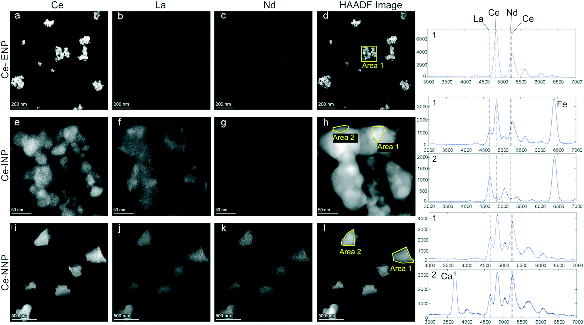 | ||
| Fig. 1 Elemental distribution maps of Ce, La, and Nd for CeO2 Ce-ENPs (a–c), ferrocerium lighter Ce-INPs (e–g), and bastnaesite/parisite Ce-NNPs (i–k). HAADF images (d, h and l) of the respective particle type show the morphology of individual particles. EDX spectra of the areas indicated are provided to the right of the images. The positions of the (main) X-ray lines for Ce, La, Nd, Ca, and Fe are labeled. | ||
The Ce-INPs formed fractal-like aggregates consisting of primary particles of only a few to a few tens of nanometers in width. REEs detected in these particles were limited to Ce and La. Within individual Ce-INPs, these REEs were separated in two phases: a Ce-rich phase forming close to spherical particles with diameters up to a few tens of nanometers and a La-rich phase that seems to flow around the Ce-rich phase (see Fig. S1†). The La-rich phase was likely present as a fluid either during the production of the mischmetal or during the spark formation. The REE-phase separation is distinct to the Ce-INPs and indicates that the Ce:La mass ratio of the Ce-INPs will likely show considerable variability.
The sampled Ce-NNPs form angular fragments from a hundred to a few hundred nanometers in diameter. Two types of Ce-NNPs, which can be distinguished by their Ca content, were observed in the Ce-NNP sample. This is consistent with two distinct mineral phases observed on backscattered electron images and elemental analyses of resin embedded bastnaesite/parisite mineral grains extracted from a host rock (see Fig. S2†). The nominal formula of bastnaesite is CeCO3F, and that of parisite is CaCe2(CO3)2F2; in both minerals, Ce can be substituted with other LREEs.26,27 In the samples examined, Ce, La, and Nd were all detected and evenly distributed in both the bastnaesite and parisite phases of the Ce-NNPs (Fig. 1i–k).
Single and multi-metal Ce-NP types
The REE contents in Ce-ENPs, Ce-INPs, and Ce-NNPs show distinct compositions, which we exploited to classify individual particles by spICP-TOFMS. All Ce-NPs contain Ce signals above the critical value (Lc,sp,Ce), but other REEs are present at variable quantities in each particle type. In Fig. 2, we plot the distributions of Ce signals recorded from stock suspensions of the Ce-ENPs (CeO2), Ce-INPs (ferrocerium lighter particles), and Ce-NNPs (ground bastnaesite/parisite minerals) as a function of the additional elements measured in each particle. All signal intensities are reported in TOF counts, as determined by instrument parameters and detector tuning. This signal will be referred to as “counts” for the rest of the manuscript. As seen in Fig. 2, the counts of Ce overlap for all single metal Ce-NPs (sm-Ce NPs). However, as the number of elements recorded in multi-metal Ce-NPs (mm-Ce NPs) increases, the average signal from Ce also increases. These count distributions show that for all Ce-NP types, a count threshold of Ce can be set, at which a unique elemental fingerprint is recorded for each NP type. Regardless of counts of Ce, only sm-Ce NPs are measured from Ce-ENPs, as expected because CeO2 does not contain measurable amounts of other REEs. From Ce-INPs, we measure both sm-Ce NPs and mm-Ce NPs with both Ce and La. At high enough counts of Ce, the only type of particle measured is mm-Ce–La NPs, making La a useful element to differentiate Ce-ENPs from Ce-INPs. From Ce-NNPs, we measure sm-Ce NPs, mm-Ce NPs with Ce and La, and mm-Ce NPs that contain additional REEs (namely Nd, Pr, and Th). At high enough Ce counts, only mm-Ce NPs with REEs are measured, making the presence of Nd, Pr, or Th advantageous to differentiating Ce-INPs from Ce-NNPs.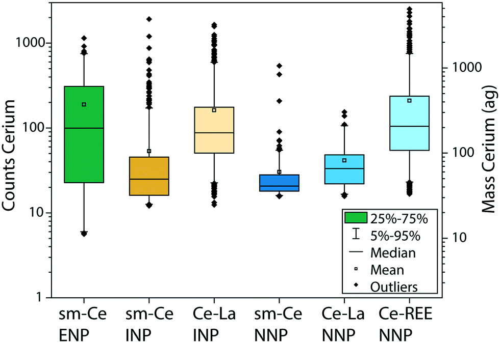 | ||
| Fig. 2 Box-and-whisker plots of Ce signals (in counts and attograms of Ce) in each NP-type are further divided based on measured elemental compositions. All Ce-NP types result in detected sm-Ce NP events. From Ce-INPs, we also record mm-Ce–La NP events. From Ce-NNPs, we record both mm-Ce–La and mm-Ce–REE particles. The mm-Ce–REE NP category includes all Ce-NNPs that had a REE (e.g., Nd, Pr, and/or Th) detected, with or without La. | ||
The average signal intensity of Ce is larger in mm-Ce NPs than in sm-Ce NPs for both the Ce-INPs and Ce-NNPs. This is a characteristic of the spICP-TOFMS measurement rather than a property of the measured particles. To detect NPs in spICP-TOFMS, the particle generated signal must be above the Lc,sp for each isotope/element measured. In particles—even those with constant mass ratios—elements with higher abundance will be measurable as particle size decreases but low-abundance elements will fall below the Lc,sp. If an element is below the Lc,sp it will not be detected, and this leads to small mm-NPs being falsely characterized as sm-NPs. In our measurements, Ce and La have roughly equal sensitivities, but Ce is more abundant, and so smaller NPs are occasionally detected as sm-Ce NPs.
In Fig. 3, we present mass correlation plots of Ce:La (Fig. 3a) and Ce:Nd (Fig. 3b) in Ce-NNPs and Ce:La (Fig. 3c) in Ce-INPs. The correlations between Ce and the other two elements in the Ce-NPs suggests that the ratios of Ce to La and Ce to Nd are conserved at the single-particle level. Scatter at low La and Ce masses is a product of measurement statistics, as described in the next section. From linear fits of the correlation plots, we determine the mass ratios of Ce:La and Ce:Nd in Ce-NNPs to be 2.1:1 and 2.2:1, respectively. This matches closely to previously measured mass ratios of ∼2:1 Ce:La and ∼2.3:1 Ce:Nd, which are known to be well-conserved in soil matrices.19,44,45 We do not record measurable amounts of Nd from Ce-INPs; however, the similarity of the Ce:La mass ratio to Ce-NNPs emphasizes that classification of these NPs by spICP-MS based on Ce–La alone is inadequate. We observe higher variation in the Ce:La mass ratios from the Ce-INPs compared to Ce-NNPs, which agrees with the results from the electron microscopy investigations showing an uneven distribution of Ce and La at the individual particle level (Fig. S1†). We will focus on the heterogeneity of this ratio in detail as it affects the accuracy of classifying our chosen Ce-NPs. In the ESI,† we provide mass spectra of these three Ce-NP types (Fig. S3†), and the ternary plots of the Ce–La–Nd contents in both Ce-NNPs and Ce-INPs (Fig. S4†).
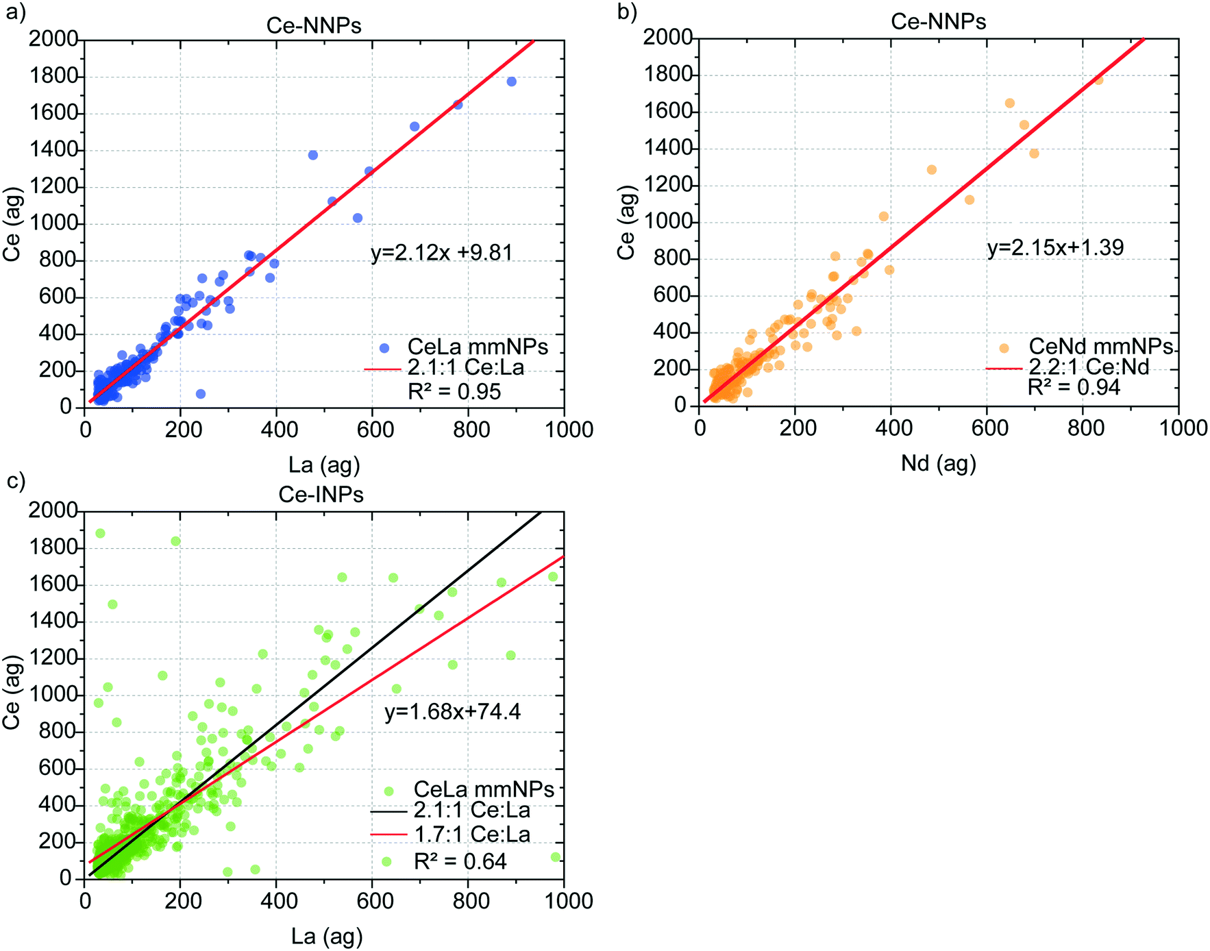 | ||
| Fig. 3 Mass correlation plots of Ce vs. La (a) and Ce vs. Nd (b) in individual Ce-NNPs and Ce vs. La in Ce-INPs (c) are plotted along with linear fits for each sample set (red line). In the Ce-NNP mass correlations, Ce is 2.1 and 2.2-times more abundant than La and Nd, respectively. More variance in the mass ratio of Ce:La in Ce-INPs is observed compared to that of the Ce-NNPs, shown by the increased spread of the particles around the mass-ratio linear fit. In (c) we also provide 2.1:1 Ce:La fit from the Ce-NNPs (black line). | ||
Poisson distribution of element ratios in Ce-NNPs
In Ce-NNPs, Ce:La and Ce:Nd mass ratios are positively correlated, and the variance of measured ratios decreases as the mass per particle of Ce, La, and Nd increases (Fig. 3). To evaluate the origin of the variation in these ratios, we plot the signal ratios of Ce:La and Ce:Nd in counts versus the recorded counts of Ce from each particle event (Fig. 4). The count ratios obtained are specific to the isotopes listed for each element in Table S4.† By plotting data in terms of counts, we can directly compare measured results to that predicted by Poisson statistics.46 Poisson statistics, used for counting methods in set intervals, describes how to predict the probability of event occurrence as a function of the mean count rate (λ). As seen in Fig. 4, the variation in signal ratios of both Ce:La and Ce:Nd follow that predicted by Poisson statistics. In Fig. 4, the confidence intervals (CI) are generated using a Poisson–normal approximation of (λ)1/2 = σ, where σ is the standard deviation, and Z-scores for a normal distribution are used. Confidence bands were created for one and two standard deviations away from the mean ratio (given the counts of Ce, La, and Nd). The CI bands are centered around mean count ratios of 2.4:1 for Ce:La and 4.1:1 for Ce:Nd. For both ratios, a few outliers extend beyond the 95% CI. These elevated-ratio outliers are due to limitations of the Poisson–normal approximations at low λ values. At low count rates Poisson distributions are right skewed, and more exact Poisson confidence intervals can be numerically calculated via Monte Carlo methods or estimated,47,48 but in this study, we found the Poisson–Normal approximation fit-for-purpose (Table S9†). Errors in Ce:La and Ce:Nd ratios follow Poisson statistics which indicate the accuracy of these ratios is controlled by our measurement technique rather than by the variation in the composition of individual Ce-NNPs. This is in congruence with the uniform distribution of the individual REEs shown by the elemental distribution maps from TEM analysis (Fig. 1). Within the sensitivity range of the spICP-TOFMS measurement, the composition of all Ce-NNPs is constant. Importantly, with measurement uncertainty controlled by Poisson statistics, we can define the statistical likelihood of measuring La or Nd in a Ce-NNP based on the recorded counts of Ce.
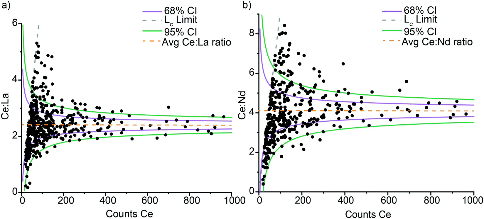 | ||
| Fig. 4 Signal ratios—Ce:La (a) and Ce:Nd (b)—from Ce-NNPs are plotted against the recorded counts of Ce in each mm-NP event. These ratios follow estimated Poisson–Normal error; pink confidence interval (CI) bands for 68% CI (±1σ) and the green bands for 95% CI (±1.96σ) contain most of the particle events. The dashed lines represent the maximum Ce:La and Ce:Nd ratios possible as a function of counts Ce and the Lc,sp for La and Nd, respectively. The ratio plots converge to average ratios of 2.4:1 (Ce:La) and 4.1:1 (Ce:Nd). | ||
Ce-NP classification method
A flow-chart depicting our Ce-NP classification scheme is provided in Fig. 5. Our scheme depends on the element composition of the Ce-NP types as well as the effective size (mass) of the individual particles. Ce-ENPs are characterized by measurable amounts of Ce in the absence of other REEs (i.e., as sm-Ce NPs). Ce-INPs are characterized by measurable amounts of Ce and La in the absence of other REEs (i.e., as mm-Ce–La NPs). Ce-NNPs are characterized by measurable amounts of Ce, La, and other REEs such as Nd. Because Ce is the most abundant element in each type, small sm-Ce NPs particles can be detected from all particle types. Likewise, mm-Ce–La NPs with low counts of Ce can be recorded from Ce-NNPs and Ce-INPs. To reduce the chance of recording false positive sm-Ce NPs or mm-Ce–La NPs events due to particle size effects, we introduce particle-type-specific detection limits (LD) for Ce-containing single particles (sp,Ce) in which detection thresholds for Ce are determined by secondary elements (Ce–La or Ce–Nd). Detection limits for Ce particles determined by La and Nd are referred to as LD,sp,Ce,Ce–La and LD,sp,Ce,Ce–Nd. These detection limits define the minimum amount of Ce counts needed to determine, with a certain confidence, whether La or Nd will be detected in a particle of a given size (mass). If the Ce signal is at or above this detection limit, we can be certain that La and Nd would be detected if the particle is truly a Ce-NNP. Detection-limit filtering allows us to classify Ce-ENP, Ce-INPs, and Ce-NNPs with reduced potential for false-positive Ce-NP classifications. The mm-Ce NP detection limits are derived from Poisson–normal statistics and utilize the constant count ratios of Ce:La and Ce:Nd in the natural particles. The LD's are also controlled by the minimum detectable sp-signal for the elements, i.e., LC,sp,Ce, LC,sp,La, and LC,sp,Nd. From LD,sp,Ce,Ce–La and LD,sp,Ce,Ce–Nd, we can create mass and size-detection limits for classification of Ce-NPs; however, these LD's are first established in terms of counts as that is the domain of Poisson statistics.
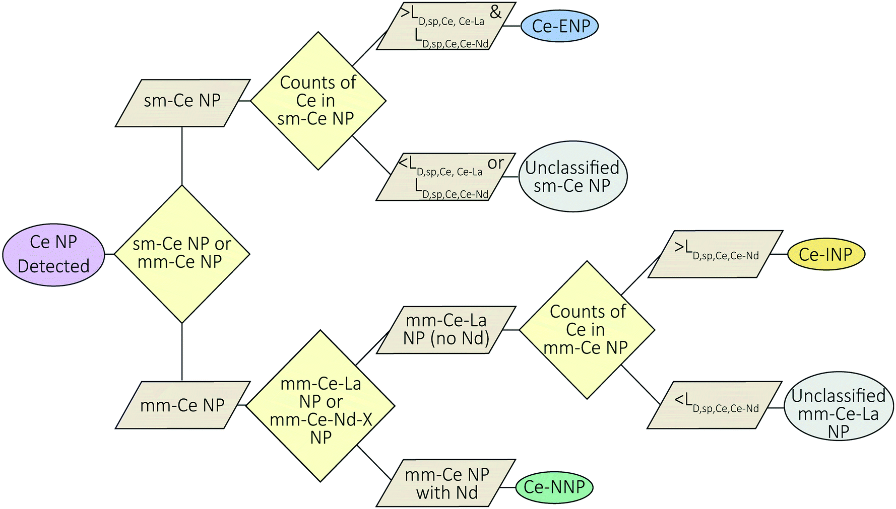 | ||
| Fig. 5 Flow chart for the classification of Ce-NP particles. | ||
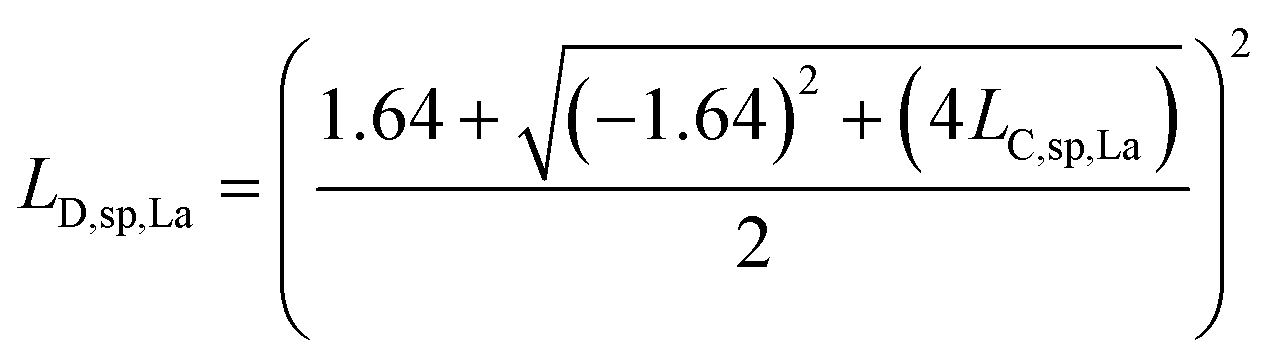
L D,sp,Ce,Ce–La and LD,sp,Ce,Ce–Nd are defined in single particles as the likelihood of measuring each element (e.g., La and Nd) as a function of the counts recorded for Ce. For simplicity, we will limit the discussion to the determination of LD,sp,Ce,Ce–La. To detect La in a particle, its signal must be above the Lc,sp,La. We use the Lc,sp,La to define the average counts of La (λ) in a recorded La signal distribution with a given false-negative rate (β). β is the fraction of the La-signal distribution below Lc,sp,La. The average counts of La is the detection limit for La (LD,sp,La) (eqn (1)); the calculation for LD,sp,La is analogous to a conventional detection limit calculation49,50 except the critical value for detection is defined independently as Lc,sp,La (eqn (2)). Eqn (3) relates LD,sp,La to a user-defined β, here set to 5% (0.05), where z1−β is the Z-score for a Normal distribution. As previously stated, the standard deviation is related to the square root of the mean count rate (λ1/2).
| LD,sp,La = λLa | (1) |
| LD,sp,La = LC,sp,La + (z1−β)(λLa)1/2 | (2) |
| z1−β = 1.64 | (3) |
| LD,sp,La = LC,sp,La + 1.64(LD,sp,La)1/2 | (4) |
 | (5) |
:La in Ce-NNPs (RCe:La) as shown in eqn (6).| LD,sp,Ce,Ce–La = (LD,sp,La)RCe:La | (6) |
:La to be 2.4:1 and use eqn (6) to set LD,sp,Ce,Ce–La = 40 counts, as shown by the blue line in Fig. 6. If the single-particle critical value for Ce (LC,sp,Ce) is below the calculated LD,sp,Ce,Ce–La, eqn (6) remains valid. The detection-limit for Ce in particles is controlled by Lc,sp,La since Ce and La have similar sensitivities and La is less abundant in Ce-NNPs. To determine LD,sp,Ce,Ce–Nd at a given false-negative rate, the above steps are repeated the using Lc,sp,Nd and RCe:Nd in place of the La-specific values.
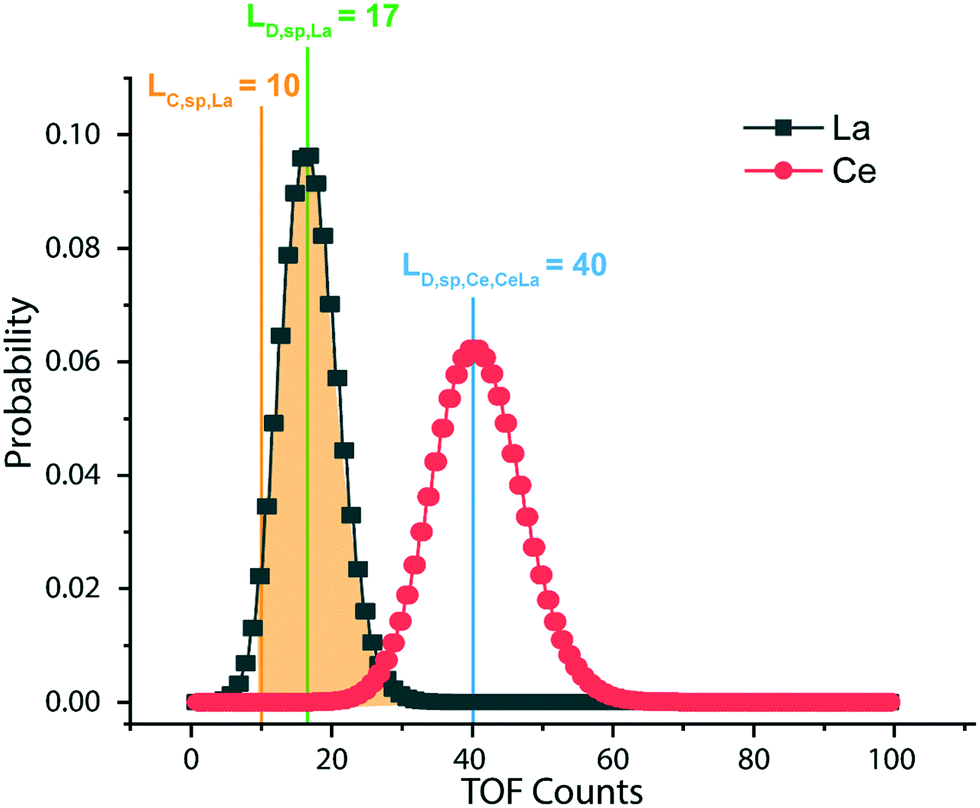 | ||
| Fig. 6 Detection limits for mm-Ce–La NPs are a function of the critical value of La (Lc,sp,La) as well as the ratio of Ce:La as controlled by Poisson statistics. Here, the detection limit for a Ce–La NP (Lc,sp,Ce,Ce–La) is the average Ce signal that leads to 95% (β = 0.05) of the La signal distribution to be above Lc,sp,La. | ||
Setting particle-type-specific detection limits for Ce and filtering Ce-NP signals with these detection limits reduces the chance of falsely classifying Ce-NP types. For example, if a sm-Ce NP is recorded and its Ce-signal is greater than both LD,sp,Ce,Ce–La and LD,sp,Ce,Ce–Nd, then we are 95% certain that we would have measured La and Nd if these elements were present in the particle, and therefore we can classify this particle as a Ce-ENP. In a case in which a mm-Ce–La NP is recorded and the Ce-signal is greater than LD,sp,Ce,Ce–Nd, then we are 95% certain that we would have measured Nd if it was present, and the particle can be confidently classified as a Ce-INP. Because Ce-ENPs and Ce-INPs do not contain measurable amounts of Nd, any particle in which Nd is detected is classified as a Ce-NNP. All sm-Ce NPs or mm-Ce–La NPs with Ce signals below LD,sp,Ce,Ce–La and/or LD,sp,Ce,Ce–Nd are deemed unclassified by this scheme, as the counts are too low to determine whether La and/or Nd are present but undetected. Essential to our classification approach is that the user can define their tolerance for false-positive classification by adjusting β, which controls the confidence interval (CI) for the detection limits according to eqn (7).
| CI = 1 − β | (7) |
Setting the CI at lower values allows for more particles to be identified, but at the cost of an increase in false positives. Setting the CI at a higher value reduces false-positive particle assignments, but will increase LD,sp,Ce,Ce–La and LD,sp,Ce,Ce–Nd, and thus result in more unclassified particles (i.e., false negatives). Here, we suggest that a CI of 95% provides a good balance of classifying many Ce-NPs without high false-positive percentages.
Single-particle-ICP-TOFMS classifications of Ce-NP stocks
For initial validation of our classification approach, we classified Ce-particle signals from stock suspensions of Ce-ENPs, Ce-INPs, and Ce-NNPs. For each of these samples, we know how all particle events should be classified and can quantify false-positive and false-negative percentages. In Fig. S4,† we report the fraction of each NP type classified from the stock suspensions both in terms of number fraction and mass fraction. For all particle types, particle-number based classification accuracy is lower than that calculated based on particle mass. Particle-type-specific LD,sp filtering removes low-mass particles that are not reliably fingerprinted, which can result in many small unclassified particles. However, if greater sensitivities could be achieved to improve the detection of smaller particles, LD,sp filtering would still be applicable. While confidence intervals for particle classification are based on Poisson statistics, the true recorded percentage of false-positive Ce-NP classification is also a function of the size (i.e. mass) distributions of the Ce-NPs in a measurement. LD,sp values are based entirely on LC,sp values and elemental ratios, and not on the size distribution of the particle population. If the size distribution of a population of particles has a mean at, or above, the size set by LD,sp, it is predicted ≥95% of the particles will be correctly classified. If the mean of the size distribution is below the LD,sp diameter, the true percent false-positives will be more than 5% because the particle size distribution is skewed toward small sizes.Ce-NNPs may be misclassified as Ce-ENPs or Ce-INPs due to the detection of sm-Ce NPs or mm-Ce–La NPs. From the stock Ce-NNPs, we classified over 70% of all Ce-NPs detected. 95% of these particles were correctly classified as Ce-NNPs while only 5% were classified as false-positive Ce-ENPs or Ce-INPs. Of the total Ce mass in all Ce-NPs detected, 93% was correctly classified. Ce-INPs are challenging to classify because, as evidenced from the TEM measurements, Ce:La ratios in individual particles are more variable than in the Ce-NNPs. Since sm-Ce NPs are detected along with mm-Ce–La NPs, misclassification as Ce-ENPs can occur. Ce-INPs cannot be misclassified as Ce-NNPs due to the absence of Nd. From our stock suspension of Ce-INPs, 48% of Ce-NPs detected were classified. 75% of these particles were correctly classified as Ce-INPs while 25% were false-positive classifications as Ce-ENPs. In terms of total Ce-NP mass, we correctly classified 72% of the Ce-mass as Ce-INPs. Ce-ENPs cannot be misclassified as Ce-INPs or Ce-NNPs because they do not contain measurable amounts of La or Nd. From our stock suspension of Ce-ENPs, we classified 60% of particles with no false positives. The Ce-mass recovery from classified Ce-ENPs was >95%. In Table S6,† we estimate the minimum classifiable size for Ce-ENP, Ce-INP, and Ce-NNPs particles based on LD,sp,Ce,Ce–La and LD,sp,Ce,Ce–Nd values from the Ce-NNP stock suspension. Assuming spherical geometry, known density, and known Ce mass fractions, size-based detection limits for Ce-ENPs, Ce-INPs, and Ce-NNPs are 31.5, 34.9, and 44.8 nm, respectively.
Classification of Ce-ENPs, Ce-INPs, and Ce-NNPs in mixtures
We used mixtures of Ce-ENPs, Ce-INPs, and Ce-NNPs to evaluate our Ce-NP classification scheme and determine figures of merit for our approach. In the first experiment, varying concentrations of Ce-ENPs and Ce-INPs were spiked into two Ce-NNP suspensions: one with a low Ce-NNP PNC and the other with a high Ce-NNP PNC. Results are presented in Fig. 7 as the number of particles classified of each Ce-NP type against the number ratios of anthropogenic Ce-NPs to Ce-NNPs. Using a high Ce-NNP background we were able to better represent real-world PNCs because in soil and water samples, Ce-NNPs will likely be at much higher PNCs than anthropogenic particles.7 Using both Ce-NNP backgrounds also enabled us to extend the dynamic range of classification. Fig. 7 shows the linear trends of both classified amounts of Ce-INPs and Ce-ENPs across samples at each dilution. For Ce-INP classification the INP:NNP particle number ratios span from 1:119 to 11:1 and for Ce-ENP classification, the ENP:NNP ratios cover 1:27 to 26:1, meaning both anthropogenic Ce-NP types can be identified against a Ce-NNP background across at least two orders of magnitude. The number of Ce-INPs that were classified ranged from 3 to 249, and Ce-ENPs ranged from 6 to 611. With increasing numbers of Ce-ENPs and Ce-INPs, the number of classified Ce-NNPs remains constant for all runs in both Ce-NNP concentrations. On average, 24 and 360 Ce-NNPs were classified for the low and high Ce-NNP matrices, respectively. While we classified down to particle ratios of 1:119 for Ce-INP:Ce-NNP, this was likely due to false positive classifications from Ce-NNPs, and from stock suspensions of Ce-NNPs, we estimate true number ratios around 1:50, or 2% false positive Ce-INPs from Ce-NNPs.
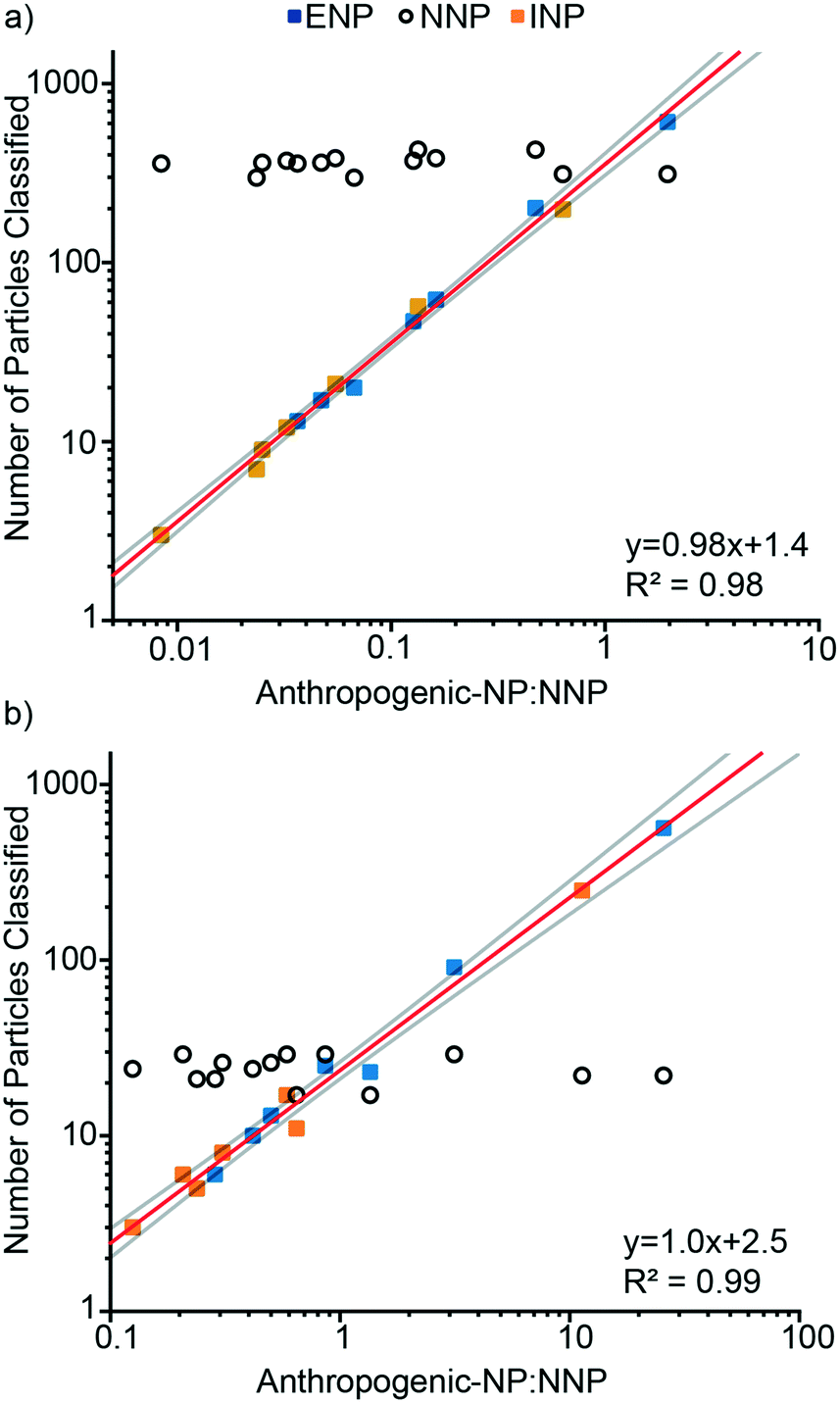 | ||
| Fig. 7 The number of particles classified of each particle type are plotted as a function of the ratio of anthropogenic-NPs to Ce-NNPs. A total of seven samples with increasing ratios of both Ce-ENPs and Ce-INPs were measured against a high Ce-NNP background (a) and a low Ce-NNP background (b). In both matrices, the amount of Ce-NNPs detected remained stable with an average of 360 Ce-NNPs in (a) and 24 Ce-NNPs in (b). Total INP:NNP ratios ranged from ∼1:119 to ∼28:1 while total ENP:NNP ratios ranged from ∼1:27 to ∼26:1. Linear trends (red lines) from increasing anthropogenic-NPs were calculated for both sets of experiments. Upper and lower 95% confidence interval lines (gray) around the trend are also provided. | ||
Because particle classification depends on single-particle critical values (LC,sp), the fraction of classifiable particles increases as the dissolved element backgrounds are reduced. Classification can be improved with increased dilution of the samples, but at the expense of measurement time. Interestingly, in this experimental data, it was observed that an increase in Ce-INP PNC was accompanied by an increase in the background of “dissolved” Ce and La signals. Results from TEM investigations show Ce-INPs with diameters around 20 nm, which are too small for quantitative detection by our spICP-TOFMS method. These small nanoparticles are detected at counts below the LC,sp values and therefore may contribute to the background signal, which raises LC,sp values for Ce and La. Increases in these critical values elevate LD,sp,Ce,Ce–La and thus increase the minimum size needed to classify particles.
In the second set of experiments, the influence of Ce-NP types on accurate classification of the other particle types was explored. In these experiments, we kept the particle number concentration of one type of anthropogenic Ce-NP constant while increasing the other; Ce-NNPs were constant in every sample. In Fig. 8, we show the particle numbers of each classified Ce-NP plotted against the dilution of the Ce-NP type as well as the linear trends for all Ce-NP types.
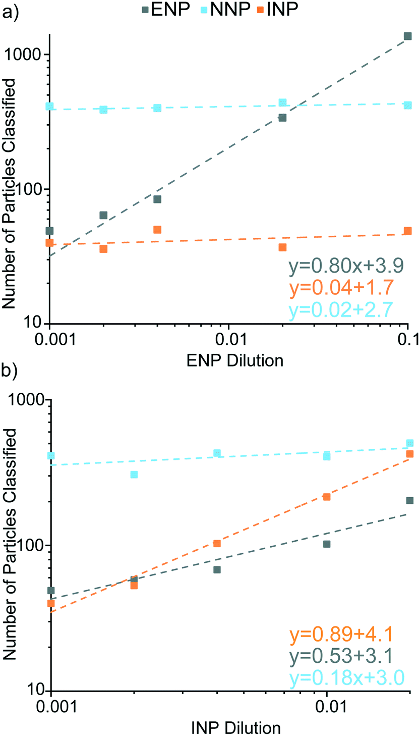 | ||
| Fig. 8 Results of the analysis of Ce-NP mixtures with constant Ce-NNP concentrations and dilutions of Ce-ENPs and Ce-INPs are plotted as the number of Ce-NPs classified vs. the dilution amount. As seen in (a), increased concentrations of Ce-ENPs (while PNC of Ce-INPs is held constant) does not lead to false positives for Ce-INPs or Ce-NNPs. In (b), concentration of Ce-INPs is increased while that of Ce-ENP remains constant. The statistical significance of each slope was tested using linear regression with a 95% confidence interval. In (a) only the slope of Ce-ENPs is significantly different than zero. In (b), the slope of the Ce-INPs is significantly different than zero. The slope of the Ce-ENPs in (b) is also significantly different than zero, but not linearly correlated with the increased concentration of in Ce-INPs. The classification of Ce-INPs directly affects classification of Ce-ENPs, and both are seen to increase, even though Ce-ENP PNC is constant. | ||
As seen in Fig. 8a, increasing the concentrations of Ce-ENPs does not result in false-positive classification of either Ce-INPs or Ce-NNPs. We also find that the Ce-background is not appreciably raised with increasing Ce-ENP concentration: LD,sp,Ce,Ce–La only changes ±3 counts across the five samples. When Ce-INP concentration increases, the dissolved background increases for both Ce and La, increasing LC,sp,Ce, LC,sp,La, and LD,sp,Ce,Ce–La values. The detection limit for Ce-INP classification (LD,sp,Ce,Ce–La) increases from 56.7 to 81.9 counts (low-to-high Ce-INP concentration), which corresponds to the detection limit in Ce mass increasing from 111 ag to 160 ag. Background elevations by Ce-INPs do not affect the Nd background, though, and Ce-NNPs are able to be classified consistently in Ce-INP backgrounds, as shown in Fig. S6.†
Ferrocerium lighter particles cause more false-positive Ce-ENP classifications than the Ce-NNPs due to the inherent heterogeneity of Ce:La in the Ce-INPs. LD,sp,Ce,Ce–La is based on the conserved ratios of Ce:La in the Ce-NNPs and this ratio is not as well-conserved in the Ce-INPs. A portion of Ce-INPs with Ce signal above LD,sp,Ce,Ce–La will contain amounts of La below the Lc,sp,La. These low-La Ce-INPs are falsely classified as Ce-ENPs. As shown in Fig. 8b, with increasing concentrations of Ce-INPs, we observe that false-positive Ce-ENPs also increase, though at a slower rate than correctly classified Ce-INPs. Falsely classifying Ce-INPs as Ce-ENPs is a limitation of our approach and is due to the variation of Ce:La in our Ce-INPs. At lower number fractions of Ce-ENPs, false-positive Ce-ENP events from Ce-INPs could outnumber true Ce-ENP events. Ce-INPs do not cause false-positive Ce-NNP events because no Nd signal is recorded from Ce-INPs.
To decrease false-positive classifications of Ce-ENPs from Ce-INPs, we must increase LD,sp,Ce,Ce–La. This can be done in two ways: either by choosing a higher confidence interval or by increasing RCe:La used for classification. For example, increasing the CI from 95% to 99% raises the LD,sp,Ce,Ce–La from 51.3 to 61.3 counts. This reduces false positives, but also reduces the percent of particles classified overall. Table S7† shows how the LD,sp counts increase for the same sample as the CI is increased. Likewise, by increasing RCe:La to a higher value, such as RCe:La = 3, the number of false-positive Ce-ENPs can be reduced at the expense of more false-negative classifications. Fig. S7† shows data displayed in Fig. 8 with Ce-ENPs re-classified using RCe:La = 3. The probability of recording false-positive Ce-ENP or Ce-INP events from either Ce-INPs or Ce-NNPs depends on the size-distribution of the measured particles, the average element ratios of the particles, and the variability of these ratios.
The ferrocerium lighter Ce-INPs used in these experiments serve as a model for other INP types that may resemble natural particles. It is likely Ce-INPs found in the environment will have Ce:La ratios that differ from the ferrocerium INPs studied here and may not resemble ratios of other coexistent NNPs. However, natural colloids have been reported to have well-conserved Ce:La and Ce:Nd ratios, which indicates that the use of these ratios is a good benchmark for Ce-NNP identification. In Table S8,† we report the single-particle Ce:La and Ce:Nd mass ratios for the Ce-containing minerals monazite, allanite, and bastnaesite/parisite, as well as from two ferrocerium-produced Ce-INP populations. From this initial analysis of Ce-containing minerals, it appears that mass ratios of 2.3–3.3 for Ce:La and 1.2–2.3 for Ce:Nd are appropriate for establishing the LD,sp values necessary for fingerprinting a range of Ce-NNP types. As more Ce-INPs are discovered, further classification categories of Ce-NPs, with Ce above the LD,sp values set by Ce-NNPs, may be incorporated.
Conclusion
Using spICP-TOFMS, we classify individual Ce-particles from three origins using mixtures of natural bastnaesite/parisite Ce-NNPs, ferrocerium lighter “flint” Ce-INPs, and CeO2 Ce-ENPs. We developed a particle-type-specific detection limit that is based in Poisson statistics to accurately classify individual single and multi-metal NPs. In our samples, individual particles are identified by the detection of Ce and the likelihood of other REEs, such as La and Nd, being detected based on the counts of Ce. Particle-type detection-limit filtering relies on single-particle critical values and the known element ratios of Ce to other REEs in Ce-NNPs.With this approach, we show mixtures of Ce-ENPs, Ce-INPs, and Ce-NNPs are quantifiable across at least three orders of magnitude. However, since Ce-NNPs inherently produce some false-positive Ce-INP and Ce-ENP classifications, we are limited to detection of number ratios down to ∼1:50 (2% false positives), for both Ce-INP:Ce-NNPs and Ce-ENP:Ce-NNPs. Our study serves as a baseline for how spICP-TOFMS data can be detection-limit filtered to provide a population of classifiable particles and reduce false-positive particle assignments.
We also report a new class of Ce-INPs, created from sparking a ferrocerium lighter, with similar Ce:La mass ratios as the Ce-NNPs used. These Ce-INPs therefore require a third element, in this case Nd, to avoid misidentification. Using our detection limit filtering, we are able to identify Ce-INPs in mixtures with Ce-NNPs. This lays the groundwork for expanding upon identifying other Ce-INPs that may be currently misclassified as natural.
Our methods can be adapted to other natural NNPs with conserved element ratios, such as minerals containing Mg, Al, Ti, Fe, or Zn. While not pursued here, detection-limit filtering could also be used for robust mineralogical assignment of different particles based on element ratios, even for particles that contain the same major and minor elements. The experiments presented in this paper represent ideal suspensions of Ce-NPs; in future work we will expand the application of this classification scheme to quantify Ce-minerals in environmental samples.
Conflicts of interest
The authors have no conflicts of interest to declare.Acknowledgements
The authors would like to acknowledge funding through a faculty start-up grant from Iowa State University. We also acknowledge Trond Forre of the Chemistry Department Glass Shop and the ISU Chemistry Machine Shop for fabrication of the microdroplet introduction system.References
- R. Gupta and H. Xie, J. Environ. Pathol., Toxicol. Oncol., 2018, 37, 209–230 CrossRef PubMed.
- W. J. Stark, P. R. Stoessel, W. Wohlleben and A. Hafner, Chem. Soc. Rev., 2015, 44, 5793–5805 RSC.
- M. Baalousha, Y. Yang, M. E. Vance, B. P. Colman, S. McNeal, J. Xu, J. Blaszczak, M. Steele, E. Bernhardt and M. F. Hochella, Jr., Sci. Total Environ., 2016, 557–558, 740–753 CrossRef CAS PubMed.
- E. Inshakova and O. Inshakov, MATEC Web Conf., 2017, 129, 02013 CrossRef.
- A. Malakar, S. R. Kanel, C. Ray, D. D. Snow and M. N. Nadagouda, Sci. Total Environ., 2021, 759, 143470 CrossRef CAS PubMed.
- F. Gottschalk, T. Sun and B. Nowack, Environ. Pollut., 2013, 181, 287–300 CrossRef CAS PubMed.
- A. A. Keller and A. Lazareva, Environ. Sci. Technol. Lett., 2014, 1, 65–70 CrossRef CAS.
- Q. Abbas, B. Yousaf, Amina, M. U. Ali, M. A. M. Munir, A. El-Naggar, J. Rinklebe and M. Naushad, Environ. Int., 2020, 138, 105646 CrossRef CAS PubMed.
- P. Westerhoff, A. Atkinson, J. Fortner, M. S. Wong, J. Zimmerman, J. Gardea-Torresdey, J. Ranville and P. Herckes, Nat. Nanotechnol., 2018, 13, 661–669 CrossRef CAS PubMed.
- L. N. Rand, K. Flores, N. Sharma, J. Gardea-Torresdey and P. Westerhoff, ACS ES&T Water, 2021, 1, 2242–2250 Search PubMed.
- A. Gogos, J. Wielinski, A. Voegelin, F. von der Kammer and R. Kaegi, Water Res.: X, 2020, 9, 100059 CAS.
- A. P. Gondikas, F. von der Kammer, R. B. Reed, S. Wagner, J. F. Ranville and T. Hofmann, Environ. Sci. Technol., 2014, 48, 5415–5422 CrossRef CAS PubMed.
- F. Laborda, E. Bolea and J. Jiménez-Lamana, Anal. Chem., 2014, 86, 2270–2278 CrossRef CAS PubMed.
- D. M. Mitrano, A. Barber, A. Bednar, P. Westerhoff, C. P. Higgins and J. F. Ranville, J. Anal. At. Spectrom., 2012, 27, 1131–1142 RSC.
- L. Hendriks, A. Gundlach-Graham and D. Gunther, Chimia, 2018, 72, 221–226 CrossRef CAS PubMed.
- A. Gundlach-Graham, in Comprehensive Analytical Chemistry, ed. R. Milačič, J. Ščančar, H. Goenaga-Infante and J. Vidmar, Elsevier, 2021, ch. 3, vol. 93, pp. 69–101 Search PubMed.
- K. Mehrabi, R. Kaegi, D. Günther and A. Gundlach-Graham, Environ. Sci.: Nano, 2021, 8, 1211–1225 RSC.
- J. Navratilova, A. Praetorius, A. Gondikas, W. Fabienke, F. von der Kammer and T. Hofmann, Int. J. Environ. Res. Public Health, 2015, 12, 15756–15768 CrossRef CAS PubMed.
- A. Praetorius, A. Gundlach-Graham, E. Goldberg, W. Fabienke, J. Navratilova, A. Gondikas, R. Kaegi, D. Günther, T. Hofmann and F. von der Kammer, Environ. Sci.: Nano, 2017, 4, 307–314 RSC.
- A. Gondikas, F. von der Kammer, R. Kaegi, O. Borovinskaya, E. Neubauer, J. Navratilova, A. Praetorius, G. Cornelis and T. Hofmann, Environ. Sci.: Nano, 2018, 5, 313–326 RSC.
- A. Azimzada, I. Jreije, M. Hadioui, P. Shaw, J. M. Farner and K. J. Wilkinson, Environ. Sci. Technol., 2021, 55, 9836–9844 CrossRef CAS PubMed.
- S. Naasz, S. Weigel, O. Borovinskaya, A. Serva, C. Cascio, A. K. Undas, F. C. Simeone, H. J. P. Marvin and R. J. B. Peters, J. Anal. At. Spectrom., 2018, 33, 835–845 RSC.
- D. Mozhayeva and C. Engelhard, J. Anal. At. Spectrom., 2020, 35, 1740–1783 RSC.
- O. Borovinskaya, S. Gschwind, B. Hattendorf, M. Tanner and D. Günther, Anal. Chem., 2014, 86, 8142–8148 CrossRef CAS PubMed.
- L. Hendriks, A. Gundlach-Graham, B. Hattendorf and D. Günther, J. Anal. At. Spectrom., 2017, 32, 548–561 RSC.
- H. I. o. Mineralogy, Bastnasite, https://www.mindat.org/min-563.html, (accessed July, 2021).
- H. I. o. Mineralogy, Parisite - (Ce), https://www.mindat.org/min-3120.html, (accessed July, 2021).
- J. T. Dahle and Y. Arai, Int. J. Environ. Res. Public Health, 2015, 12, 1253–1278 CrossRef PubMed.
- K. Reinhardt and H. Winkler, Ullmann's Encycl. Ind. Chem., 2000 DOI:10.1002/14356007.a06_139.
- M. F. Hochella, Jr., D. W. Mogk, J. Ranville, I. C. Allen, G. W. Luther, L. C. Marr, B. P. McGrail, M. Murayama, N. P. Qafoku, K. M. Rosso, N. Sahai, P. A. Schroeder, P. Vikesland, P. Westerhoff and Y. Yang, Science, 2019, 363, 6434 CrossRef PubMed.
- K. Phalyvong, Y. Sivry, H. Pauwels, A. Gélabert, M. Tharaud, G. Wille, X. Bourrat and M. F. Benedetti, Front. Environ. Sci., 2020, 8 DOI:10.3389/fenvs.2020.00141.
- C. Xu and X. Qu, NPG Asia Mater., 2014, 6, 90 CrossRef.
- A. Laycock, B. Coles, K. Kreissig and M. Rehkämper, J. Anal. At. Spectrom., 2016, 31, 297–302 RSC.
- M. D. Montaño, H. R. Badiei, S. Bazargan and J. F. Ranville, Environ. Sci.: Nano, 2014, 1, 338–346 RSC.
- F. von der Kammer, P. L. Ferguson, P. A. Holden, A. Masion, K. R. Rogers, S. J. Klaine, A. A. Koelmans, N. Horne and J. M. Unrine, Environ. Toxicol. Chem., 2012, 31, 32–49 CrossRef CAS PubMed.
- T. R. Holbrook, D. Gallot-Duval, T. Reemtsma and S. Wagner, J. Anal. At. Spectrom., 2021, 36, 2684–2694 RSC.
- H. H. Meng and C. H. Lin, Forensic Sci. Int., 2008, 7, 37–44 Search PubMed.
- K. Mehrabi, D. Günther and A. Gundlach-Graham, Environ. Sci.: Nano, 2019, 6, 3349–3358 RSC.
- A. Gundlach-Graham and K. Mehrabi, J. Anal. At. Spectrom., 2020, 35, 1727–1739 RSC.
- H. E. Pace, N. J. Rogers, C. Jarolimek, V. A. Coleman, C. P. Higgins and J. F. Ranville, Anal. Chem., 2011, 83, 9361–9369 CrossRef CAS PubMed.
- A. Gundlach-Graham, L. Hendriks, K. Mehrabi and D. Günther, Anal. Chem., 2018, 90, 11847–11855 CrossRef CAS PubMed.
- L. Hendriks, A. Gundlach-Graham and D. Günther, J. Anal. At. Spectrom., 2019, 34, 1900–1909 RSC.
- R. Kaegi, M. Fierz and B. Hattendorf, Microsc. Microanal., 2021, 27, 557–565 CrossRef CAS PubMed.
- W. Yao, X. Xie and X. Wang, Geosci. Front., 2011, 2, 247–259 CrossRef CAS.
- EuroGeoSurveys, Geochemical Atlas of Europe, http://weppi.gtk.fi/publ/foregsatlas/index.php, (accessed August, 2021).
- S. Yamashita, M. Ishida, T. Suzuki, M. Nakazato and T. Hirata, Spectrochim. Acta, Part B, 2020, 169, 105881 CrossRef CAS.
- L. Barker, Am. Stat., 2002, 56, 85–89 CrossRef.
- E. L. Crow and R. S. Gardner, Biometrika, 1959, 46, 441–453 CrossRef.
- L. A. Currie, Anal. Chem., 1968, 40, 586–593 CrossRef CAS.
- L. A. Currie, Pure Appl. Chem., 1995, 67, 1699–1723 CrossRef CAS.
Footnote |
| † Electronic supplementary information (ESI) available. See DOI: 10.1039/d1en01039e |
| This journal is © The Royal Society of Chemistry 2022 |