
Controls on the epilimnetic phosphorus concentration in small temperate lakes†
Aria
Amirbahman‡
 *a,
Kaci N.
Fitzgibbon
b,
Stephen A.
Norton
b,
Linda C.
Bacon
c and
Sean D.
Birkel
bde
*a,
Kaci N.
Fitzgibbon
b,
Stephen A.
Norton
b,
Linda C.
Bacon
c and
Sean D.
Birkel
bde
aDepartment of Civil and Environmental Engineering, University of Maine, Orono, Maine 04469, USA. E-mail: aamirbahman@scu.edu
bSchool of Earth and Climate Sciences, University of Maine, Orono, Maine 04469, USA
cThe Maine Department of Environmental Protection, Augusta, Maine 04333, USA
dClimate Change Institute, University of Maine, Orono, Maine 04469, USA
eUniversity of Maine Cooperative Extension, Orono, Maine 04469, USA
First published on 8th December 2021
Abstract
Phosphorus (P) is one of the key limiting nutrients for algal growth in most fresh surface waters. Understanding the determinants of P accumulation in the water column of lakes of interest, and the prediction of its concentration is important to water quality managers and other stakeholders. We hypothesized that lake physicochemical, climate, and watershed land-use attributes control lake P concentration. We collected relevant data from 126 lakes in Maine, USA, to determine the major drivers for summer total epilimnetic P concentrations. Predictive regression-based models featured lake external and internal drivers. The most important land-use driver was the extent of agriculture in the watershed. Lake average depth was the most important physical driver, with shallow lakes being most susceptible to high P concentrations; shallow lakes often stratify weakly and are most subject to internal mixing. The sediment NaOH-extracted aluminum (Al) to bicarbonate/dithionite-extracted P molar ratio was the most important sediment chemical driver; lakes with a high hypolimnetic P release have low ratios. The dissolved organic carbon (DOC) concentration was an important water column chemical driver; lakes having a high DOC concentration generally had higher epilimnetic P concentrations. Precipitation and temperature, two important climate/weather variables, were not significant drivers of epilimnetic P in the predictive models. Because lake depth and sediment quality are fixed in the short-term, the modeling framework serves as a quantitative lake management tool for stakeholders to assess the vulnerability of individual lakes to watershed development, particularly agriculture. The model also enables decisions for sustainable development in the watershed and lake remediation if sediment quality is conducive to internal P release. The findings of this study may be applied to bloom metrics more directly to support lake and watershed management actions.
Environmental significanceUnderstanding the drivers of lake eutrophication and loss of water quality is important for sustainability of aquatic ecosystems. This work identifies and quantifies the effect of such drivers on the epilimnetic phosphorus concentration in 126 Maine, USA, lakes. The results show that lake physicochemical, climate, and watershed land-use attributes control lake phosphorus concentration. The models developed here can serve as management decision tools for public agencies and other stakeholders to assess lake vulnerability to eutrophication. |
1. Introduction
Temperate regions of North America and Europe have abundant lakes, the majority of which are smaller than 2.5 km2.1 These lakes perform important ecosystem functions: they are home to a diversity of flora and fauna, provide various ecosystem services, and have a great impact on local and state economies. For example, Boyle et al.2 reported that lakes in Maine, USA, contributed approximately $5 billion to the state economy; this value has nearly doubled by 2021. These lakes are also less resilient to external stimuli and can undergo loss of water quality faster than larger lakes. Most of these lakes have excess phosphorus (P) availability as the leading cause of eutrophication and loss of water quality.3 P flux into a lake is seasonally variable and can be external from the watershed, and/or internal, when externally added P is recycled from the sediment within the lake. Effective management of lake water quality requires a fundamental understanding of physical and chemical factors that lead to cultural eutrophication. Quantification of such underlying factors also allows the successful development of models to predict lake vulnerability to eutrophication. Aquatic nutrient cycling research and modeling is especially timely given the growing threat of harmful algal blooms (HABs).4 HABs are not restricted to eutrophic lakes, but can also occur in low-nutrient lakes, including those in temperate regions.5–8The classic ‘input–output’ models for P, introduced by Vollenweider,9 rely on estimates of watershed point and non-point source export to assess lake P loading. Anthropogenic activity, particularly agricultural development in the watershed, increases the sediment and nutrient loads to a lake through application of fertilizers and increased soil erosion, making watershed land-use and hydrology important variables. Phosphorus can also originate from the dissolution of apatite (Ca5(PO4)3(OH)), the most abundant P-containing primary mineral in boreal ecosystems, and via transport of DOC, and particulate Al(OH)3 and Fe(OH)3 with adsorbed P.10
Although important, knowledge of external P inputs to a lake is insufficient to evaluate vulnerability to eutrophication and should be augmented with data from in-lake and climate/weather-related factors. Lakes that develop summer hypolimnetic anoxia may be subject to internal P loading via sediment P release that has also been reported due to anoxic condition even in shallow areas.11 The classic model of sediment P release involves the microbially-catalyzed reductive dissolution of sediment Fe(OH)3 as the predominant mechanism.12–16 In oxic sediments, Fe(OH)3 binds orthophosphate strongly, but upon its dissolution, the adsorbed P is released and becomes bioavailable to algae as it reaches the photic zone. However, excess sediment Al(OH)3 can effectively sequester P and inhibit its release to the overlying water despite anoxia.17–20 P sequestration by Al(OH)3 occurs in low pH, low P lakes.21 Al(OH)3, in contrast to Fe(OH)3, is not redox-sensitive, and therefore, P adsorption to Al(OH)3 is unaffected under anoxic condition. Thermodynamically, P adsorption onto Fe(OH)3 surface is favored over that of Al(OH)3. Equilibrium adsorption, however, is not only controlled by thermodynamics, but also by the concentration of surface adsorption sites. Therefore, excess Al(OH)3 can provide sufficient surface sites to effectively compete with the Fe(OH)3 surface for adsorption. Indeed, soluble Al salts, such as alum, have commonly been added as a lake management strategy to prevent internal P release.22
The sequential chemical extraction procedure developed by Psenner et al.23 allows the fractionation of sediment P, Fe, and Al into exchangeable (NH4Cl), reducible (Na bicarbonate-dithionite; BD), and NaOH- and HCl-extractable fractions. Laboratory experiments and field observations showed that lakes with sediment molar ratios of AlBD+NaOH![[thin space (1/6-em)]](https://www.rsc.org/images/entities/char_2009.gif) :FeBD (henceforth Al:Fe) >3 and AlBD+NaOH:PBD (henceforth Al:P) >25 release a negligible amount of hypolimnetic P during summer anoxia, indicating that an increase in sediment extractable Al concentration leads to sequestration of sediment P.17,24
:FeBD (henceforth Al:Fe) >3 and AlBD+NaOH:PBD (henceforth Al:P) >25 release a negligible amount of hypolimnetic P during summer anoxia, indicating that an increase in sediment extractable Al concentration leads to sequestration of sediment P.17,24
Characteristics other than land use and geochemistry influence the effect of external loading on the lake P budget. The watershed area to lake area ratio (WA:LA) has been used as a metric to characterize watershed contribution with respect to nutrient loading in a lake.25,26 The studies reported a positive correlation between lake P and WA:LA. Further, Huser et al.22 found that WA:LA correlated negatively and significantly with hydraulic residence time (HRT), a variable that has been used as a metric to characterize the role of hydrology in lake water quality modeling.9 Specifically, HRT correlates negatively with the external P flux into the lake.27
Lake water quality is also influenced by lake morphometry, including depth and surface area that, along with water temperature, affect lake thermal structure and strength of stratification.28,29 In strongly stratified lakes, characterized by relatively large decreases in temperature and increasing density with depth, mass transfer between hypolimnetic and epilimnetic waters is slow; consequently, seasonal increases in high hypolimnetic P in these stable lakes may not result in simultaneous increases in the epilimnetic P.30 However, lakes with negligible thermal stability, especially shallow lakes that experience ephemeral anoxia in their metalimnia, are more susceptible to mixing by wind. In shallow lakes, entrainment of the bottom water may happen frequently,31 potentially leading to higher epilimnetic P concentrations.32
Lake thermal stability has been implicated as a factor influencing the occurrence of HABs.33 Increased thermal stability in the water column, brought about by increased air temperature, decreased wind speed, and decreased cloudiness can reduce the vertical turbulent mixing, favoring the buoyant cyanobacteria over other species of phytoplankton.34
We hypothesize that (a) lake physiochemical characteristics, (b) climate/weather characteristics, and (c) watershed/land use characteristics strongly influence lake epilimnetic P concentration. We have used relevant data from 126 lakes in Maine, USA (Tables S1 and S2†),35 to test our hypotheses and develop models that predict lake P concentrations based on the above drivers of lake water quality. We developed regression-based models based on 98 of these lakes for which complete data existed that incorporate various components of watershed, lake (including the direct role of sediment chemistry with respect to P mobilization), and climate/weather characteristics to estimate lake summer total epilimnetic P. In particular, incorporating variables that represent sediment chemistry along with other established measures, such as lake depth and extent of agriculture, into predictive models for lake water quality is unique to our knowledge. These models are especially appropriate for studies that inform stakeholders, guide regional efforts to maintain lake water quality by managing land use, and aim to remediate high internal P loading.
2. Methodology
2.1. Field sites
The lakes in this study were sampled in 2010–2012 (90 by the Maine Department of Environmental Protection; DEP), 2013 (12 by the Lakes Environmental Association), and 2015 (24 by Fitzgibbon35), using the same techniques everywhere. All lakes are predominantly located in the southern and central regions of Maine (Fig. S2†), and were sampled in the months of July, August, or early September in a few cases. These are the period of maximum stratification in Maine. All data are in Tables S1, S2† and Fitzgibbon.352.2. Sampling and analysis
Water and sediment samples were obtained from the deepest point in each lake. Dissolved oxygen (DO) and temperature were measured in 1–2 m increments from the surface to 1 m from the sediment surface. Integrated epilimnetic core water samples were collected using a flexible PPE sampling tube from the lake surface to 1 m below the bottom of the epilimnion. Water samples from the hypolimnion were collected with a Kemmerer grab sampler from 1 m above the sediment–water interface. Samples were collected for closed-cell pH and total P in all lakes. Samples for anions (SO42−, NO3−, Cl−), unfiltered total cations (Ca, Mg, Na, K, Al, and Fe), and dissolved organic carbon (DOC) were collected for a subset of lakes. Closed-cell pH was measured with a TitraLab TIM860 Titration Manager. Total (unfiltered) P (henceforth P) was measured with a Varian Cary 50 spectrophotometer using a molybdate blue coloring reagent following ammonium peroxydisulfate digestion (250 °C, 0.5 h). Ion chromatography (Dionex DX-500) was used to analyze the anions. Cation samples were acidified with 50% HNO3 to a pH <2 in the field. A high resolution ICP-MS (Thermo Element 2) was used to measure cation concentrations. For quality control, blank, replicate, and analyte-spiked samples were run every 10 water samples; the error was within 5% for all samples and analytes.Sediment samples were obtained using a Hongve-style gravity corer.36 Sediment samples from the top 2 cm were composited from three cores collected within a 3 m radius and kept frozen in the dark until analysis. Diagenetic processes in the sediment alter the speciation and concentrations of P, Al, and Fe.14 Thus, we limited our focus to the top 2 cm of sediment with an age of probably <10 years. It is largely this interval of sediment that interacts most with hypolimnetic water (or epilimnetic water in shallow lakes) during anoxia.
The sediment sequential extraction procedure was a modified version of Psenner et al.23 The first (ion-exchangeable fraction) was omitted because several studies on Maine lake sediments indicated that the typical extractable Al, Fe, and P concentrations in the first extraction step were <1% of those of the second and third extraction steps (e.g., Lake et al.24). The third extraction step was modified from Psenner et al.23 by using 0.1 M NaOH, rather than 1 M NaOH.18 We also eliminated the fifth extraction step (total residual extractable fraction) because this high temperature extraction (85 °C) with 1 M NaOH removes only very insoluble material that is not biologically available.
Two grams of wet sediment were sequentially extracted with 25 ml of solution of (a) 0.11 M Na bicarbonate (NaHCO3) and 0.11 M Na dithionite (NaS2O4) at 40 °C for 30 min to extract reducible Fe (FeBD) and the associated P (PBD) via the reductive dissolution of Fe(OH)3; (b) 0.1 M NaOH at 25 °C for 16 h to extract Al (AlNaOH) via the dissolution of Al(OH)3, and P (PNaOH) that is largely associated with Al(OH)3 and organic matter; and (c) 0.5 M HCl at 25 °C for 16 h to extract P associated with any calcite (CaCO3) or apatite present,17 as well as the less soluble Al(OH)3 and Fe(OH)3 phases that did not dissolve in the previous two extraction steps. Calcite was not observed in the sediment of any of these soft water and generally low-P lakes, based on the relatively low extracted Ca2+ concentrations in the HCl sediment extracts and lack of proportionality of Ca2+ and P.35 Lakes in Maine, as a group, are comparatively low in Ca2+ and Mg2+ because of low amounts of limestone (CaCO3) and/or rapidly weathering lithologies in the bedrock and glacial materials. In Maine, apatite occurs commonly in post-glacial marine and lake sediment below an elevation of 75 m ASL near the coast, rising to 128 m inland.37
Acidic deposition, starting in earnest after WWII, peaking in the early 1970s and then declining, has had long-term effects on water and sediment chemistry of Maine lakes. However, this study was not designed to specifically address lake responses to recovery from acid rain in Maine (ubiquitous but originally of declining strength from southwest to northeast), or other spatially discontinuous influences that typically have shorter recoveries than from acid rain, including fire, cycles of drought followed by acidic pulses of runoff, pest invasion with defoliation, altered land use, forestry harvesting practices, changing DOC, and climate changes. The latter, also ubiquitous, include higher temperatures and more intense rainfall events with higher annual totals, all well documented.38 Of course, it is possible that short-lived events disproportionately impacted surface sediment chemistry of a lake, but most lake catchments were chosen based on relatively little or no recent land-based disturbance. The spatial breadth (nearly state-wide), short sampling period (2010–2015), and large number of lakes in this study provide a snapshot of recent water and sediment chemistry.
Concentrations of P, Al, Fe, and Ca in the sediment extracts were determined using inductively coupled plasma atomic emission spectrometry (ICP-AES; Thermo Element 2). For quality control, blank and replicate samples were run for every 10 field samples, with typical variability of <5%.
2.3. Calculated variables and watershed information
Several variables that reflect lake physical characteristics were calculated. Lake area-averaged depth (Zavg) considers the lake morphometry as,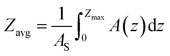 | (1) |
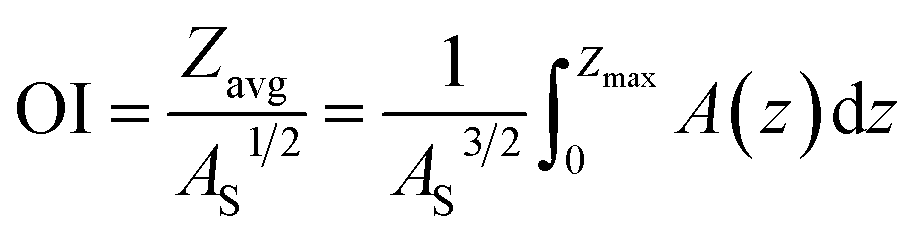 | (2) |
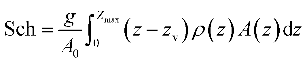
A measure of a lake's thermal stability, the Schmidt stability, Sch (J m−2), is the energy required to mix a unit area of a lake to a uniform water density,40
 | (3) |
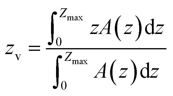 | (4) |
Lakes with a high Sch are less susceptible to physical mixing than those with a low Sch. In thermally stable lakes (i.e., a high Sch value), the density difference between the epilimnion and hypolimnion is sufficient to counteract the shear forces created by wind. Sch does not explicitly account for wind velocity, even though the destabilizing effect of wind is implicitly included in the homogenization of the density gradient.41 We used the rLakeAnalyzer package v. 3.3 to calculate Sch (Global Lake Ecological Observatory Network; http://www.gleon.org/).
Stream Stats (https://water.usgs.gov/osw/streamstats/) from the United States Geological Survey (USGS) was used to access lake watershed information that included the percentage of storage for the water bodies and associated wetlands (from the National Wetlands Inventory), and the mean basin slope, which was computed from the 10 m digital elevation model (DEM) from Stream Stats (https://www.nrcs.usda.gov/wps/portal/nrcs/detail/soils/survey/). Lake area included contiguous wetlands. Maine Office of GIS's (MEGIS; http://www.maine.gov/megis/) GeoLibrary was accessed to acquire the land cover spatial data in each watershed35 from the Maine Land Cover Dataset (MELCD; http://www.maine.gov/megis/catalog/metadata/melcd.html#ID0EUEA), a land cover map derived from Landsat Thematic Mapper 5 and 7 from the years 1999–2000. Spatial data were collected with a resolution of 30 m. We used SPOT 5 panchromatic imagery from 2004 to refine this map. The SPOT 5 imagery was collected with a spatial resolution of 5 m.
The effect of agriculture on lake epilimnetic P was assessed by determining the hay/pasture plus cultivated crop land area in watersheds and dividing by the watershed or lake area to obtain agricultural land:watershed area ratio (Ag:WA) and agricultural land:lake area ratio (Ag:LA), respectively. We also considered the contribution of the agricultural land contiguous with the lake to obtain the adjacent agricultural land:watershed area ratio (AdjAg:WA).
Daily precipitation (maximum, average, and sum) and temperature (degree-day) data from January 1st and May 1st to the sampling date in the same year were collected to assess their influence on epilimnetic P. The data at each lake latitude/longitude center point were obtained from the Parameter-Elevation Regressions on Independent Slopes Model (PRISM).42,43 PRISM is a statistical mapping system that uses in situ point measurements to generate high-resolution spatial climate solutions using a digital elevation model and a weighted regression scheme. Gridded data products, such as PRISM, offer an ideal means to obtain climate estimates over areas where local observations are not available. In this study, we used the 4 km × 4 km PRISM solutions downloaded from the PRISM Climate Group.44
2.4. Statistical analysis
Multiple linear regression (MLR) models were developed and ranked to provide a predictive tool for the epilimnetic P concentrations, given a set of predictor variables. Variables whose variances did not meet the assumptions of normality and homogeneity were log transformed. The level of multicollinearity among the predictor variables was determined by calculating the variance inflation factor (VIF); a cutoff value of 2 was used above which predictor variables were not included. The corrected Akaike information criterion (AICC) was used as a means for model selection. The AICC estimates the relative quality of the models for a data set by accounting for a limited sample size, with the lowest AICC indicating the highest quality. The models are ranked based on the maximum likelihood and minimum number of predictor variables. The ΔAICC of a model is the difference between AICC of that model and the model with the lowest AICC. Models are considered of equal quality when ΔAICC <2, while ΔAICC >10 denotes models that are significantly different.45 An estimate of the predictor variables for the MLR models was provided by performing a regression tree analysis (see the ESI section†). The MLR analysis was performed using the R package Hmisc.Quantile regression (QR) models were developed to explore the response of epilimnetic P concentration to agricultural development for a top multiple regression model across different quantiles. QR models are generally utilized to provide a more comprehensive description of the relationship among variables by estimating the conditional quantiles of the response variable distribution.46 This technique estimates the conditional quantiles of the response variable as a function of the predictor variable; the 50th quantile (τ = 0.50) corresponds to the conditional median, where 50% of the lakes have equal or less than a specified epilimnetic P concentration. Compared to linear least squares models, QR models have the advantage of reducing the influence of uncharacterized predictor variables on the response variable by estimating functional relations across the entire range of the probability distribution. This is especially important when the slope of the regression line differs for different quantiles.47
Quantile regression was further used in conjunction with percentile selection, as defined by Xu et al.,48 to develop specific P management strategies for agricultural development. Specifically, they used this approach to analyze the response of lake chlorophyll to N and P concentrations, and set management targets for these nutrients. Different percentiles of concentrations of one nutrient were chosen and QR analysis was performed for each set of percentiles to fit the relationship between chlorophyll and other nutrients by the 99th quantile model. The QR models for each set of nutrient percentiles were used to predict the concentration of other nutrient that would reach the threshold chlorophyll target of 15 μg L−1. We used this approach, in particular, to estimate the extent of agricultural development in a watershed in response to a threshold epilimnetic P concentration under ranked sediment Al:P ratios and Zavg, two of the specific lake characteristics that control epilimnetic P concentrations. QR analysis was performed using the R package quantreg (2016), v. 5.26.
3. Results and discussion
Based on our hypothesis that determinants of lake water quality include in-lake physiochemical characteristics, climate/weather factors, and watershed/land use characteristics, we chose several measured and calculated variables, including those related to lake morphometry, and sediment and water chemistry to represent these categories.3.1. Physicochemical controls
| logEpiP |
logHypoP |
logAl:P |
logPBD |
logAl:Fe |
Ag:WA |
AdjAg:LA |
WA:LA |
Ag:LA |
Road:WA | Z avg | T hyp | logSch |
OI | pH | DOC | |
|---|---|---|---|---|---|---|---|---|---|---|---|---|---|---|---|---|
|
a EpiP (μg L−1): epilimnetic P; HypoP: hypolimnetic P; Al:P: sediment AlBD+NaOH:PBD molar ratio; PBD (μmol g−1): sediment P extracted in bicarbonate-dithionite extraction; Al:Fe: sediment AlBD+NaOH:FeBD molar ratio; Ag:WA: %agricultural area:watershed area; AdjAg:LA: %lake adjacent agricultural area:lake surface area; WA:LA: watershed area:lake surface area ratio; Ag:LA: agricultural area:lake surface area ratio; Road:WA: road surface area:watershed area ratio; Zavg (m): area-averaged lake depth; Thyp (°C): hypolimnetic temperature 1 m above lake bed; Sch (J m−2): Schmidt Stability; OI: Osgood Index; DOC (mg L−1): dissolved organic carbon. Watershed area does not include lake area.
|
||||||||||||||||
| logEpiP |
1 | |||||||||||||||
| logHypoP |
0.700* | 1 | ||||||||||||||
| logAl:P |
−0.461* | −0.432* | 1 | |||||||||||||
| logPBD |
0.436* | 0.437* | −0.971* | 1 | ||||||||||||
| logAl:Fe |
−0.015 | −0.163 | 0.551* | −0.488* | 1 | |||||||||||
| Ag:WA |
0.540* | 0.522* | −0.515* | 0.510* | −0.269* | 1 | ||||||||||
| AdjAg:LA |
0.428* | 0.379* | −0.261* | 0.289* | −0.032 | 0.614* | 1 | |||||||||
| WA:LA |
0.087 | 0.183 | −0.041 | 0.007 | 0.010 | −0.006 | 0.066 | 1 | ||||||||
| Ag:LA |
0.466* | 0.253 | −0.298* | 0.295* | −0.138 | 0.667* | 0.449* | 0.238* | 1 | |||||||
| Road:WA |
−0.038 | 0.096 | −0.023 | 0.022 | 0.018 | 0.017 | 0.039 | −0.056 | −0.028 | 1 | ||||||
| Z avg | −0.555* | −0.358* | −0.071 | 0.098 | −0.504* | −0.163 | −0.145 | −0.108 | −0.204 | 0.013 | 1 | |||||
| T hyp | 0.456* | 0.128 | −0.009 | −0.070 | 0.088 | 0.174 | 0.021 | −0.078 | −0.206 | −0.126 | −0.636* | 1 | ||||
| logSch |
−0.376* | −0.248 | −0.144 | 0.215 | −0.289* | −0.001 | −0.090 | −0190 | −0.098 | 0.062 | 0.691* | −0.860* | 1 | |||
| OI | −0.308* | −0.146 | 0.338* | −0.288* | 0.219 | −0.230 | −0.080 | −0.091 | −0.153 | 0.044 | 0.055 | −0.383* | 0.234* | 1 | ||
| pH | 0.497* | 0.507* | −0.596* | 0.557* | −0.402* | 0.521* | 0.200 | 0.044 | 0.418* | 0.016 | −0.061 | 0.119 | 0.045 | −0.225 | 1 | |
| DOC | 0.371* | 0.216 | 0.042 | −0.077 | 0.158 | 0.066 | 0.036 | 0.225 | 0.289* | −0.110 | −0.348* | 0.372* | −0.457* | −0.187 | −0.060 | 1 |
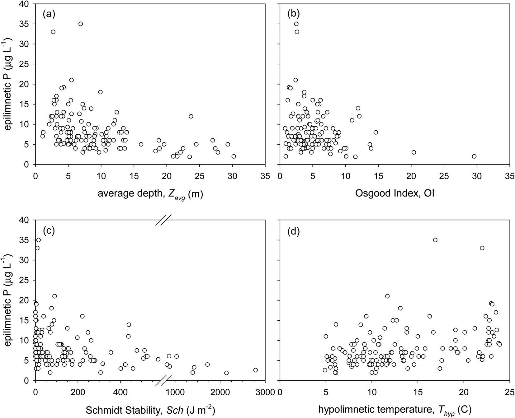 | ||
| Fig. 1 Epilimnetic P (μg L−1) versus (a) area-averaged depth (Zavg), r = −0.418; (b) Osgood Index (OI), r = −0.233; (c) Schmidt stability (Sch), r = −0.303; and (d) hypolimnetic temperature (Thyp), r = 0.399. | ||
Osgood Index, a measure of lake morphometry, has been related to lake thermal stability. Osgood39 suggested that lakes with OI >6 develop stable thermal stratification, whereas lakes with OI <6 are susceptible to summer mixing during which the epilimnetic water quality is strongly influenced by the metalimnion or hypolimnion. Our results indicate that OI is significantly negatively correlated to lake epilimnetic P (Table 1), and lakes with a high OI (>12) have low epilimnetic P concentrations (<10 μg L−1 with average = 5.7 μg L−1), whereas lakes with high epilimnetic P concentrations (>15 μg L−1) have a low OI (<7; Fig. 1b). Lakes with OI <7 have an average P concentration = 8.9 μg L−1. However, several lakes with very low OI also have very low epilimnetic P concentrations. Our observations are similar to those by Mataraza and Cooke32 who evaluated the OI for 114 temperate lakes and concluded that OI cannot be used as the only predictor for lake epilimnetic P concentrations.
Welch and Cooke30 presented cases where an increase in the summer hypolimnetic P concentration in lakes with OI >7 did not result in a similar increase in the summer epilimnetic P. Huser et al.22 observed that alum treatment longevity in temperate lakes increased significantly at OI >5.7. Clearly, shallow lakes with a low OI are more susceptible to wind-driven mixing, which allows internally released sediment P to reach the epilimnion at a faster rate. In deeper lakes with a high OI, internally released P may not reach the epilimnion rapidly, or until spring or fall overturn.
Our results show that lakes with Sch >500 J m−2 at the time of sampling have epilimnetic P concentrations <6 μg L−1 (Fig. 1c), suggesting that P-rich bottom waters migrate upward at a slower rate in thermally stratified lakes to the top in thermally stable lakes. However, in our study a large number of lakes with Sch <600 J m−2 had low epilimnetic P concentrations, indicating that similar to OI, Sch cannot be used as the only predictor of lake water quality. The yearly sum of Sch, derived from a lake physical model, may be a better indicator for the seasonal lake thermal stability and, potentially, epilimnetic P concentration.53 Lake thermal stability, as characterized by Sch, is subject to change throughout the season depending on climate and weather factors, such as rainfall intensity, persistent wind, and air and water temperature. In lakes that undergo mixing in fall and spring, such as most of those studied here, Sch reaches its maximum value prior to the fall turnover, and zero immediately after the fall and spring turnovers.
The negative correlation between Sch and epilimnetic P (Table 1) is due to the enhancement of mass transfer between hypolimnia and epilimnia in lakes with a low Sch, causing erosion of the thermocline, more frequent oxygenation of the hypolimnion, and introduction of nutrients into the epilimnion.54 Lathrop et al.29 observed a positive relationship between summer Secchi depth and Sch in a temperate lake. In a survey of 231 lakes in northeastern North America during 1975–2012, Richardson et al.55 showed that the strength of thermal stratification increases with increasing warming of surface temperatures, particularly for lakes at higher latitudes (above ∼44°), which includes most of Maine.
Similar to OI and Zavg, WA:LA may be used as an indirect measure of the hydrological landscape.22,26 A low WA:LA suggests a potentially higher percentage of internally-loaded P. Conversely, lakes with higher WA:LA ratios are likely more influenced by external P sources.25,52,56 However, in this study WA:LA was not significantly correlated to epilimnetic P and was not a determinant of epilimnetic P in the statistical analysis (Table 1).
Temperature degree-days did not correlate with the epilimnetic P in our study (Table S3†). However, epilimnetic P was positively correlated with Thyp (Table 1; Fig. 1d) and Tepi (Table S3†). Higher temperatures, especially closer to the sediment, enhance microbial activity that leads to depletion of DO and release of P due to reductive dissolution of Fe(OH)3 at the sediment–water interface.57,58 The released P may be translocated to the epilimnion depending on the lake thermal stability. A warmer hypolimnion also reduces lake thermal stability, as manifested in the strong but inverse relationship between Thyp and Sch (r = −0.86; Table 1). Even though a significant correlation was not observed between Tepi and Sch, the difference between Tepi and Thyp was strongly and positively correlated to Sch (r = 0.82), indicating that lakes with a small temperature gradient are more susceptible to mixing.
:P, positively correlated to sediment PBD, and uncorrelated with sediment Al:Fe (Table 1). Our results show that lakes with relatively high sediment Al:P ratios have lower epilimnetic P concentrations, and lakes with high epilimnetic P concentrations have relatively small ratios (Fig. 2). The insignificant internal P release in lakes with threshold sediment molar ratios of Al:Fe >3 and Al:P >25,17 however, is most clearly observed when assessed against the hypolimnetic P concentration (Fig. S3†) or its sediment hypolimnetic flux.24
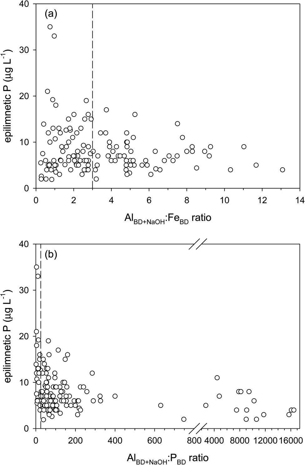 | ||
| Fig. 2 (a) Sediment AlBD+NaOH:FeBD molar ratio versus epilimnetic P (μg L−1), r = −0.162. The dashed line shows AlBD+NaOH:FeBD ratio = 3; (b) sediment Al BD+NaOH:PBD molar ratio versus epilimnetic P, r = −0.234. The dashed line shows Al BD+NaOH:PBD ratio = 25. | ||
Equilibrium adsorption depends not only on surface reaction energetics, but also by the concentration of surface adsorption sites. The sediment Al:Fe = 3 and Al:P = 25 ratios, initially established via laboratory experiments, represent threshold relative sediment Al concentrations above which P is effectively bound to the Al(OH)3 surface. At higher ratios, the Al(OH)3 surface effectively competes with the Fe(OH)3 surface for P adsorption in eroded soil,10 water column,59 and lake sediment.17 Under anoxic conditions, sediment P associated with the reducible Fe(OH)3 (i.e., PBD) is susceptible to mobilization. Al(OH)3 remains insoluble under anoxia provided that hypolimnetic pH remains between 5.5 and 8.5, and if present at sufficiently high concentrations, it can effectively prevent hypolimnetic sediment P release.17,20 In lakes with a high sediment Al content, P is permanently buried. In these lakes, the sediment total P concentration does not decrease with sediment depth, as it typically does in eutrophic lake sediments. Instead, the mineralization of organic P takes place without its significant upward diffusion into the bottom waters; i.e. P remains conservative during sediment diagenesis.14,19 Al addition to lake sediment is an established method for remediation of lakes that are subject to significant internal P cycling.22,60 The threshold sediment ratios should be considered by lake managers and other stakeholders when adding Al to remediate lake eutrophication due to excess P concentrations.
As hypothesized, the determinants of lake epilimnetic P concentrations are not limited to the sediment geochemical factors. Whereas sediment Al:Fe and Al:P ratios below the threshold values are required for sediment P release (Fig. S3†), meeting the thresholds does not result in a significant P release in some lakes. Further, even though P release may not be significant in some lakes, the ratios indicate lake vulnerability to internal P release. But, these ratios, by themselves, cannot be used for estimation of the lake internal P release, and the epilimnetic P concentration.
:P and Al:Fe ratios, suggesting enhanced mobilization of Al from the watershed with decreasing pH.65 Other processes, however, may lead to enhanced P mobilization at a lower pH. Apatite, as a source of P from many Maine watersheds and lake sediments, is more soluble at a lower pH and lower Ca2+ concentrations; however, apatite is commonly depleted in mineral soils in a few thousand years.66 Many lakes in Maine have easily and recently eroded post-glacial unweathered marine sediments containing apatite in their watersheds at elevations below 75 m ASL near the coast increasing to 128 m ASL inland.37,67 In a survey of 257 lakes in Maine with little or no agricultural development in their watersheds, 16 lakes whose watersheds were dominated by marine clay had an excess of approximately 5 μg L−1 epilimnetic P.68
The DOC concentration in our study lakes ranged from 1.7 to 8.1 mg L−1 (Table S1†). There is a weak but significant positive relationship between lake DOC and epilimnetic P (Table 1), similar to that observed for other boreal lakes.49,69,70 In our study, DOC concentrations are positively correlated with the percentage of agricultural land (Ag:LA; Table 1), and the wetland area-to-watershed area ratio.35 However, WA:LA, previously correlated to lake DOC concentration by Rasmussen et al.,71 is not significantly correlated with DOC in our study (Table 1). The magnitude of lake DOC concentration is determined by watershed land cover type, hydrological connectivity patterns, and lake HRT.72–74
In recent decades, DOC concentrations have been increasing in surface waters of Europe and North America,75 and may be rebounding to values typical of pre-acid rain times.76 DOC can transport nutrients, including P, to lakes.20 DOC may also transport Al and Fe to lakes where photo-oxidation of these complexes yields precipitated Al(OH)3 and Fe(OH)3.59 These amorphous phases may then adsorb P from the water column and become sediment. Increased DOC increases light attenuation that may result in enhanced lake stratification because of warming of shallower water, thereby decreasing the epilimnetic depth.77,78 A higher thermal stability can, in turn, diminish the translocation of hypolimnetic P to the epilimnion.31 The influence of DOC on lake nutrient cycling is complex and not fully understood,77 confusing the interpretation of its statistical relationship with epilimnetic P.
3.2. External loading: watershed characteristics and precipitation
Our results show weak but significant relationships between epilimnetic P concentrations and Ag:WA, Ag:LA, and AdjAg:LA ratios (Table 1). Other land-use and landscape features, such as areal road coverage (Road:WA, Table 1), urban development, and wetlands were considered, but did not contribute significantly to lake water quality.35
Several studies have observed a positive significant relationship between percent agricultural land use and lake nutrient concentrations, especially for lakes with no known point-source of pollution in their watersheds.50,69,79–81 Among different land-use and landscape features, % pasture has shown the strongest correlation with lake P.82,83
In temperate lakes, precipitation has been reported to negatively affect water quality due to the enhanced transport of sediment and nutrients into the lake.84,85 However, our data show a weak but significant negative relationship between maximum and average rainfall from May 1st to the time of sampling and lake epilimnetic P concentration (Table S3†). Other precipitation measures were not significantly related to epilimnetic P (Table S3†). The anomalous relationship between precipitation and the epilimnetic P concentration may be due lake-specific features. In particular, precipitation is positively correlated with the sediment Al:P ratio, and negatively correlated with agricultural development (Table S3†), two of the most important drivers of epilimnetic P (Table 1). Indeed, where present in the watershed, agriculture has been found as the most important driver of lake water clarity between dry (increased clarity) and wet years (reduced clarity).84 We also observe a relatively small range of precipitation across our study sites; the maximum and average precipitation values from May 1st to the sampling date are 38.8 ± 12.8 and 3.3 ± 0.8 mm, respectively. The role of precipitation as a climate factor on lake water quality may best be explored by following the epilimnetic P concentration over long time periods.86 This would also circumvent the complicating role of lake-specific effects.
3.3. Predictive tools for the epilimnetic P
We used the variables in Table 1 to build predictive linear models for summer epilimnetic P concentrations. We performed multiple regression analyses on 98 lakes, for which a complete dataset existed, to gain insights into relationship nuances. Linear models have been previously used to relate different lake water quality response variables to chemical, physical, watershed, and food web predictors.22,29,49,87:P, PBD, pH, DOC, and Zavg), and watershed characteristics (Ag:WA, AdjAg:LA, and Ag:LA). Further, shallow lakes are more susceptible to changes in climate and weather factors including temperature variations and storm intensity. Hence, Zavg can enhance the effects of climate change on a lake, such as the susceptibility of shallow lakes to mixing. The model coefficients consistently show that lower Al:P ratios and Zavg, and higher PBD, DOC, and agricultural development result in higher epilimnetic P concentrations (Table S4†).
:WA, and DOC are also shown for comparison
| Models | n | K | AICC | ΔAICC | −2 × LnL | exp(−ΔAICC/2) | w i | r 2 | |
|---|---|---|---|---|---|---|---|---|---|
| a Number of model-estimated variables plus the intercept and variance. b Likelihood of the specific model relative to other models. | |||||||||
| 1 | logAl:P + Zavg + %AdjAg:LA + DOC |
98 | 6 | −103.65 | 0.00 | −112.29 | 1.00 | 0.65 | 0.721 |
| 2 | logAl:P + Zavg + %Ag:WA + DOC |
98 | 6 | −101.95 | 1.70 | −110.60 | 0.43 | 0.28 | 0.712 |
| 3 | logPBD + Zavg + %AdjAg:LA + DOC |
98 | 6 | −99.02 | 4.63 | −107.67 | 0.10 | 0.06 | 0.708 |
| 4 | logAl:P + Zavg + Ag:LA + DOC |
98 | 6 | −94.77 | 8.87 | −103.42 | 0.01 | 0.01 | 0.695 |
| 5 | logAl:P + Zavg + %Ag:WA + pH |
98 | 6 | −91.50 | 12.14 | −100.15 | 0.00 | 0.001 | 0.684 |
| 6 | logAl:P + Zavg + %AdjAg:LA |
98 | 5 | −91.11 | 12.54 | −98.26 | 0.00 | 0.001 | 0.676 |
| 7 | logPBD + Zavg + %Ag:WA + pH |
98 | 6 | −89.76 | 13.89 | −98.41 | 0.00 | 0.001 | 0.678 |
| 8 | logAl:P + Zavg + %Ag:WA |
98 | 5 | −89.30 | 14.34 | −96.46 | 0.00 | 0.000 | 0.670 |
| 9 | logAl:P + Zavg + Ag:LA |
98 | 5 | −88.92 | 14.73 | −96.07 | 0.00 | 0.000 | 0.669 |
| 10 | logPBD + Zavg + %Ag:WA |
98 | 5 | −86.19 | 17.45 | −93.35 | 0.00 | 0.000 | 0.659 |
|
Z
avg + %Ag:WA + DOC |
98 | 5 | −71.49 | 32.16 | −78.64 | 0.00 | 0.00 | 0.604 | |
|
Z
avg + %Ag:WA |
98 | 4 | −64.36 | 39.29 | −70.07 | 0.00 | 0.00 | 0.565 | |
The top two models with ΔAICC <2 feature Zavg, Al:P ratio, DOC concentration, and Ag:WA or AdjAg:LA. The VIF for all predictor variables was <2. Predictor variables that represent climate/weather effects on lake water quality, including Sch, Thyp, Tepi, and the maximum and average precipitation from May 1st, did not rank sufficiently high with respect to predicting the summer epilimnetic P. However, Thyp and Sch correlate strongly with Zavg (Table 1), a prominent predictor for the epilimnetic P in all of the MLR models; the variables affected by climate conditions (Thyp and Sch) and the tendency to mixing are affected by Zavg.
Previous studies that used MLR modeling have shown a linear dependence of lake P on depth and land-use variables, such as the watershed size, and agricultural area.49–51,88 We have shown that the incorporation of sediment geochemical variables into MLR models improves model prediction of lake epilimnetic P (Table 2).
:WA in response to a threshold epilimnetic P under ranked sediment Al:P ratio and Zavg. Use of these three variables are based on results of a top MLR model with these three predictor variables (Table 2). We targeted lakes that may be more susceptible to the release of sediment reducible P, by using the lowest ranked sediment Al:P ratios. Ranked Al:P ratios ranged from 1.6 to 199 for the 75th percentile (n = 74), and 1.6 to 67 for the 50th percentile (n = 49). By ranking Zavg we targeted the shallower lakes that may be more susceptible to effects of internal P release. Ranked Zavg values ranged from 1.1 to 11.9 m for the 75th percentile, and 1.1 to 8.3 m for the 50th percentile. We did not report the 25th percentile because of the small number of data points.
We used a threshold of 15 μg L−1 (logP = 1.18) for the summer epilimnetic P as transition from mesotrophic to lower eutrophic,89 and the 90th quantile model to assess lake vulnerability with respect to agricultural development in the watershed. The 90th quantile epilimnetic P is the value where 90% of the lakes have concentrations less than or equal to the threshold of epilimnetic P = 15 μg L−1. The crossing of the 90th quantile model and the threshold P concentration denotes the predicted Ag:WA that should not be exceeded to limit the maximum epilimnetic P concentration to 15 μg L−1. The threshold value for the Ag:WA for lakes in the 75th percentile of sediment Al:P is 4.8%, and in the 50th percentile of sediment Al:P is 3.9% (Fig. 3a and b). The Ag:WA thresholds for lakes in the 75th and 50th percentiles of Zavg are 5.4% and 4.1%, respectively (Fig. 4a and b). Exceeding these threshold Ag:WA predicts >15 ppb epilimnetic P concentrations in most study lakes.
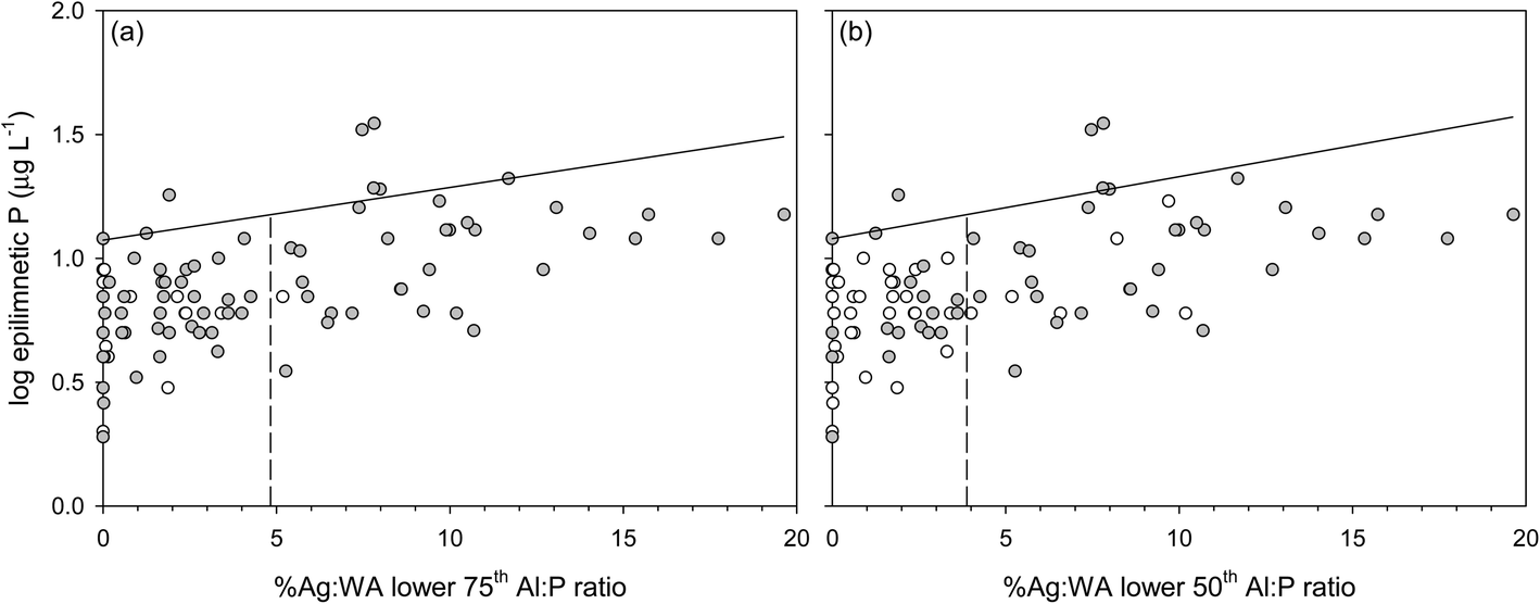 | ||
| Fig. 3 (a) %Ag:WA for the lower 75th percentile AlBD+NaOH:PBDversus logepilimnetic P (μg L−1); and (b) the lower 50th percentile AlBD+NaOH:PBDversus log epilimnetic P (μg L−1). The 90th quantile QR models (solid line) for logepilimnetic P as a function of %Ag:WA for ranked AlBD+NaOH:PBD values (75th and 50th, filled circles). The thresholds for the epilimnetic P concentrations for limiting a specific %Ag:WA target (logepilimnetic P = 1.18 corresponds to 15 μg L−1, dashed line). The open circles indicate values above the percentile of interest. The crossing of the 90th quantile model and the threshold P concentration denotes the predicted %Ag:WA that should not be exceeded to maintain an epilimnetic P concentration of 15 μg L−1 as an upper limit. | ||
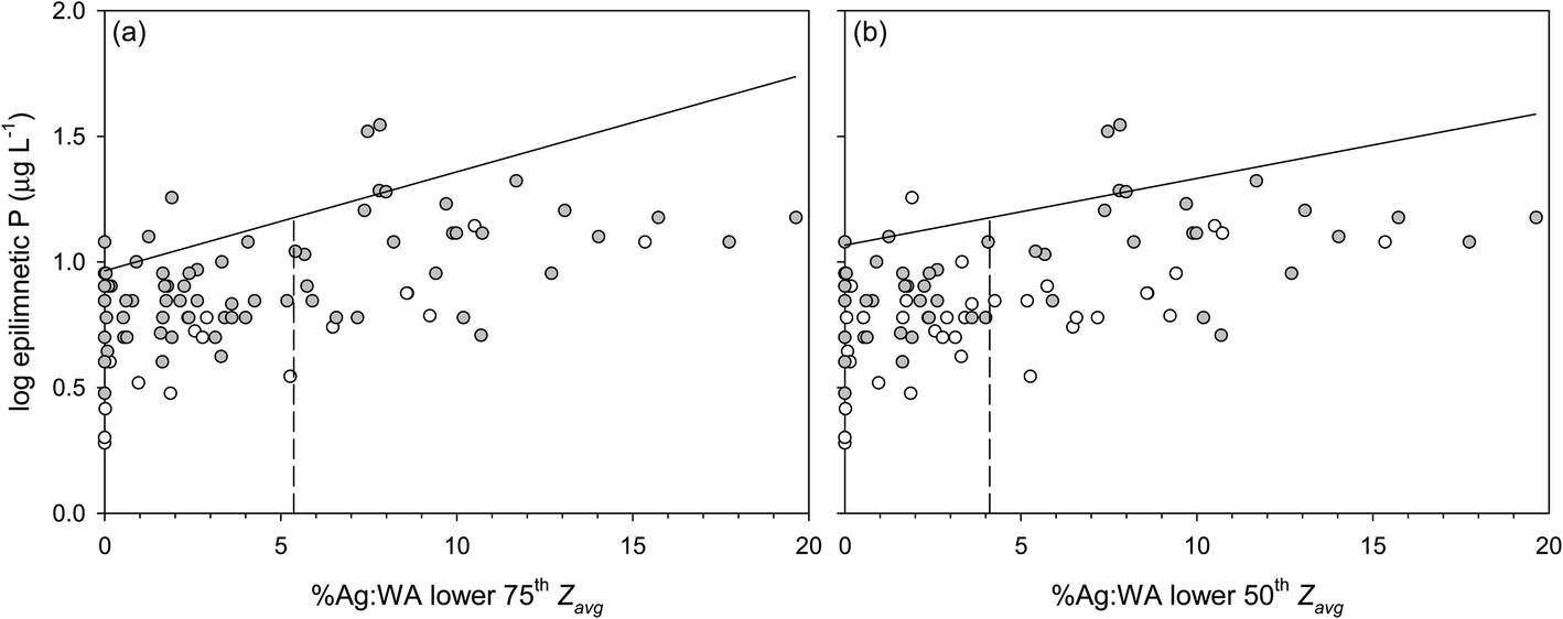 | ||
| Fig. 4 (a) %Ag:WA for the lower 75th percentile Zavgversus logepilimnetic P (μg L−1); and (b) the lower 50th percentile Zavgversus logepilimnetic P (μg L−1). The 90th quantile QR models (solid line) for logepilimnetic P as a function of %Ag:WA for ranked Zavg values (75th and 50th, filled circles). The thresholds for the epilimnetic P concentrations for limiting a specific %Ag:WA target (logepilimnetic P = 1.18 corresponds to 15 μg L−1, dashed line). The open circles indicate values above the percentile of interest. The crossing of the 90th quantile model and the threshold P concentration denotes the predicted %Ag:WA that should not be exceeded to maintain an epilimnetic P concentration of 15 μg L−1 as an upper limit. | ||
QR models relationships between predictor variables and conditional quartiles of the response variable, whereas MLR models relationships between predictor variables and conditional mean of the response variable. Significant differences between the slopes of QR and MLR models are indicative of different effects along the distribution of the response variable. In this study, however, the regression slopes at different quantiles were not significantly different than that of the MLR model (Fig. S4 and S5†). This suggests a homogeneous variance and justifies the use of the MLR model in this study.46 Our use of coupled QR and percentile selection is intended to define potential regulatory thresholds with respect to the extent of agricultural development in lake watersheds.
4. Conclusions
We have shown that lake vulnerability to eutrophication may be characterized by considering the combined effects of physiochemical, climate/weather, and watershed factors. This study identifies the determinants for epilimnetic P accumulation, and hence, variation of water quality in small temperate lakes. They are Zavg, sediment Al:P ratio, DOC concentration, and the extent of agricultural development (i.e., Ag:WA, and AdjAg:LA). Lakes with unfavorable sediment geochemistry (i.e., low molar Al:P ratios or high PBD concentrations) are more susceptible to sediment P release. Such lakes are especially vulnerable if they do not stratify stably during the summer. Shallow lakes often stratify weakly and are at a greater risk to internal mixing. Lake watershed land-use patterns determine the extent of external P contribution. Watersheds with greater areas of adjacent agriculture enhance dissolved and particulate P in surface runoff. Whereas individual factors studied here cannot be used for estimation of the epilimnetic P concentration, combined, they account for the external and internal sources of P to lakes.
The quantile regression, with percentile selection framework proposed here, sets thresholds for agricultural development that are modulated by Zavg and lake sediment Al:P ratio; exceeding the thresholds predicts epilimnetic P concentrations >15 ppb, the transition to eutrophic water quality. Such framework, by identifying determinants of epilimnetic P, informs lake managers, municipalities, and lake protection associations in how their management practices impact lake water quality.
Conflicts of interest
There are no conflicts to declare.Acknowledgements
Funding for this work was provided by grants from the U.S. National Science Foundation (CBET 1743082) and the Senator George J. Mitchell Center for Sustainability Solutions at the University of Maine. The authors are grateful to the citizen scientists and professional lake monitors, organized through the Lake Stewards of Maine and the Lake Environmental Association, for collecting water samples and lake profiles used in this research. We thank Jeffry Dennis, Jeremy Deeds, and Douglas Suitor of the Maine Department of Environmental Protection for sharing their ideas and efforts on this project, and William Halteman for his assistance in statistical analysis. Gertrud Nürnberg and two anonymous reviewers are acknowledged for their constructive comments on the manuscript.References
- J. A. Downing, Y. T. Prairie, J. J. Cole, C. M. Duarte, L. J. Travnik, R. G. Striegl, W. H. McDowell, P. Kortelainen, N. F. Caraco, J. M. Melack and J. J. Middelburg, The global abundance and size distribution of lakes, ponds, and impoundments, Limnol. Oceanogr., 2006, 51, 2388–2397 CrossRef.
- K. Boyle, J. Schuetz and J. S. Kahl, Great ponds play an integral part in Maine's economy, Water Research Institute, University of Maine, REP 473, April 1997 Search PubMed.
- D. W. Schindler, Evolution of phosphorus limitation in lakes, Science, 1977, 195, 260–262 CrossRef CAS PubMed.
- H. W. Paerl, W. S. Gardner, K. E. Havens, A. R. Joyner, M. J. McCarthy, S. E. Newell, B. Qin and J. T. Scott, Mitigating cyanobacterial harmful algal blooms in aquatic ecosystems impacted by climate change and anthropogenic nutrients, Harmful Algae, 2016, 54, 213–222 CrossRef PubMed.
- J. G. Winter, A. M. DeSellas, R. Fletcher, L. Heintsch, A. Morley, L. Nakamoto and K. Utsumi, Algal blooms in Ontario, Canada: Increases in reports since 1994, Lake Reservoir Manage., 2011, 27, 107–114 CrossRef.
- K. L. Cottingham, H. A. Ewing, M. L. Greer, C. C. Carey and K. C. Weathers, Cyanobacteria as biological drivers of lake nitrogen and phosphorus cycling, Ecosphere, 2015, 6(1) DOI:10.1890/ES14-00174.1.
- E. J. Favot, K. M. Rühland, A. M. DeSellas, R. Ingram, A. M. Paterson and J. P. Smol, Climate variability promotes unprecedented cyanobacterial blooms in a remote, oligotrophic Ontario lake: evidence from paleolimnology, Journal of Paleolimnology, 2019, 62, 31–52 CrossRef.
- H. A. Ewing, K. C. Weathers, K. L. Cottingham, P. R. Leavitt, M. L. Greer, C. C. Carey, B. G. Steele, A. U. Fiorillo and J. P. Sowles, “New” cyanobacterial blooms are not new: two centuries of lake production are related to ice cover and land use, Ecosphere, 2020, 11(6), e03170, DOI:10.1002/ecs2.3170.
- R. A. Vollenweider, Input-output models with special reference to the phosphorus loading concept in limnology, Schweizerische Zeitschrift für Hydrologie, 1975, 37, 53–84 CAS.
- M. D. SanClements, I. J. Fernandez and S. A. Norton, Soil and sediment phosphorus fractions in a forested watershed at Acadia National Park, ME, USA, For. Ecol. Manage., 2009, 258, 2318–2325 CrossRef.
- O. Tammeorg, G. Nürnberg, J. Niemistö, M. Haldna and J. Horppila, Internal phosphorus loading due to sediment anoxia in shallow areas: implications for lake aeration treatments, Aquat. Sci., 2020, 82 DOI:10.1007/s00027-020-00724-0.
- G. Nürnberg, A comparison of internal phosphorus loads in lakes with anoxic hypolimnia: Laboratory incubations versus in situ hypolimnetic phosphorus accumulation, Limnol. Oceanogr., 1987, 32, 1160–1164 CrossRef.
- H. Jensen, P. Kristensen, E. Jeppesen and A. Skytthe, Iron:phosphorus ratio in surface sediment as an indicator of phosphate release from aerobic sediments in shallow lakes, Hydrobiologia, 1992, 235/236, 731–743 CrossRef.
- T. A. Wilson, A. Amirbahman, S. A. Norton and M. A. Voytek, A record of phosphorus dynamics in oligotrophic lake sediment, Journal of Paleolimnology, 2010, 44, 279–294 CrossRef.
- A. Amirbahman, B. A. Lake and S. A. Norton, Seasonal phosphorus dynamics in the surficial sediment of two shallow temperate lakes: A solid-phase and pore-water study, Hydrobiologia, 2013, 701, 65–77 CrossRef CAS.
- G. K. Nürnberg, R. Fischer and A. M. Paterson, Reduced phosphorus retention by anoxic bottom sediments after the remediation of an industrial acidified lake area: Indications from P, Al, and Fe sediment fractions, Sci. Total Environ., 2018, 626, 412–422 CrossRef PubMed.
- J. Kopáček, J. Borovec, J. Hejzlar, K. U. Ulrich, S. A. Norton and A. Amirbahman, Aluminum control of phosphorus sorption by lake sediments, Environ. Sci. Technol., 2005, 29, 8784–8789 CrossRef PubMed.
- T. A. Wilson, S. A. Norton, B. A. Lake and A. Amirbahman, Sediment geochemistry of Al, Fe, and P for two oligotrophic Maine lakes during a period of acidification and recovery, Sci. Total Environ., 2008, 404, 269–275 CrossRef CAS PubMed.
- C. C. Carey and E. Rydin, Lake trophic status can be determined by the depth distribution of sediment phosphorus, Limnol. Oceanogr., 2011, 56, 2051–2063 CrossRef CAS.
- P. M. Homyak, J. O. Sickman and J. M. Melack, Phosphorus in sediments of high-elevation lakes in the Sierra Nevada (California): implications for internal phosphorus loading, Aquat. Sci., 2014, 76, 511–525 CrossRef CAS.
- J. Kopáček, J. Hejzlar, J. Borovec, P. Porcal and I. Kotorová, Natural inactivation of phosphorus by aluminum in atmospherically acidified water bodies, Limnol. Oceanogr., 2000, 45, 212–225 CrossRef.
- B. J. Huser, S. Egemose, H. Harper, M. Hupfer, H. Jensen, K. M. Pilgrim, K. Reitzel, E. Rydin and M. Futter, Longevity and effectiveness of aluminum addition to reduce sediment phosphorus release and restore lake water quality, Water Res., 2016, 97, 122–132 CrossRef CAS PubMed.
- R. Psenner, R. Pucsko and M. Sager, Die fraktionierung organischer und anorganischer Phosphorverbindungen von Sedimenten—versuch einer definition ökologisch wichtiger fraktionen, Arch. Hydrobiol., Suppl., 1984, 70, 111–155 CAS.
- B. A. Lake, K. M. Coolidge, S. A. Norton and A. Amirbahman, Factors contributing to the internal loading of phosphorus from anoxic sediments in six Maine, USA, lakes, Sci. Total Environ., 2007, 373, 534–541 CrossRef CAS PubMed.
- J. M. Fraterrigo and J. A. Downing, The influence of land use on lake nutrients varies with watershed transport capacity, Ecosys, 2008, 11, 1021–1034 CrossRef CAS.
- K. E. Webster, P. A. Soranno, K. S. Cheruvelil, M. T. Bremigan, J. A. Downing, P. D. Vaux, T. R. Asplund, L. C. Bacon and J. Connor, An empirical evaluation of the nutrient-color paradigm for lakes, Limnol. Oceanogr., 2008, 53, 1137–1148 CrossRef CAS.
- J. Kalff, Limnology, Prentice Hall, New Jersey, 2002 Search PubMed.
- P. A. Soranno, S. R. Carpenter and R. C. Lathrop, Internal phosphorus loading in Lake Mendota: Response to external loads and weather, Can. J. Fish. Aquat. Sci., 1997, 54, 1883–1893 CrossRef CAS.
- R. C. Lathrop, S. R. Carpenter and D. M. Robertson, Summer water clarity responses to phosphorus, Daphnia grazing, and internal mixing in Lake Mendota, Limnol. Oceanogr., 1999, 44, 137–146 CrossRef.
- E. B. Welch and G. D. Cooke, Internal phosphorus loading in shallow lakes: Importance and control, Lake Reservoir Manage., 1995, 11, 273–281 CrossRef.
- S. W. Effler, B. A. Wagner, S. M. O'Donnell, D. A. Matthews, D. M. O'Donnell, R. K. Gelda, C. M. Matthews and E. A. Cowen, An upwelling event at Onondaga Lake, NY: characterization, impact and recurrence, Hydrobiologia, 2004, 511, 185–199 CrossRef CAS.
- L. K. Mataraza and G. D. Cooke, A test of a morphometric index to predict vertical phosphorus transport in lakes, Lake Reservoir Manage., 1997, 13, 328–337 CrossRef.
- H. W. Paerl and J. Huisman, Blooms like it hot, Science, 2008, 320, 57–58 CrossRef CAS PubMed.
- K. D. Jöhnk, J. Huisman, J. Sharples, B. Sommeijer, P. M. Visser and J. M. Stroom, Summer heatwaves promote blooms of harmful cyanobacteria, Glob. Change Biol., 2008, 14, 495–512 CrossRef.
- K. N. Fitzgibbon, Evaluating Potential for Water Quality Decline in Maine Lakes, MS thesis, University of Maine, Orono, https://digitalcommons.library.umaine.edu/etd/2780, 2017.
- D. Hongve, En bunnhenter som er lett å lage, Fauna, 1972, 25, 281–283 Search PubMed.
- J. Deeds, A. Amirbahman, S. A. Norton and L. Bacon, A hydrogeomorphic and condition classification for Maine, USA, lakes, Lake Reservoir Manage., 2020, 36, 122–138 CrossRef.
- I. Fernandez, S. Birkel, C. Schmitt, J. Simonson, B. Lyon, A. Pershing, E. Stancioff, G. Jacobson and P. Mayewski, Maine's Climate Future 2020 Update, University of Maine, Orono, ME, 2020, p. 44, https://climatechange.umaine.edu/wp-content/uploads/sites/439/2020/02/Maines-Climate-Future-2020-Update-3.pdf Search PubMed.
- R. Osgood, Lake mixis and internal phosphorus dynamics, Arch. Hydrobiol., 1988, 113, 629–638 CAS.
- W. Schmidt, Über Temperatur und Stabilitätsverhältnisse von Seen, Geografiska Annaler, 1928, 10, 145–177 Search PubMed.
- D. M. Robertson and J. Imberger, Lake number, a quantitative indicator of mixing used to estimate changes in dissolved oxygen, Int. Rev. Hydrobiol., 1994, 79, 159–176 CrossRef CAS.
- C. Daly, R. P. Neilson and D. L. Phillips, A statistical topographic model for mapping climatological precipitation over mountainous terrain, J. Appl. Meteorol., 1994, 33, 140–158, DOI:10.1175/1520-0450(1994)033<0140:ASTMFM>2.0.CO;2.
- C. Daly, M. Slater, J. A. Roberti, S. Laseter and L. Swift, High-resolution precipitation mapping in a mountainous watershed: Ground truth for evaluating uncertainty in a national precipitation dataset, Int. J. Climatol., 2017, 37(suppl. 1) DOI:10.1002/joc.4986.
- PRISM Climate Group, PRISM daily time series dataset, Northwest Alliance for Computational Science and Engineering, Oregon State University, Corvallis, OR, 2020, available at: http://prism.oregonstate.edu/, accessed 10th March 2020 Search PubMed.
- K. P. Burnham and D. R. Anderson, Model Selection and Multimodel Inference: A Practical Information-Theoretic Approach, Springer-Verlag, New York, 2nd edn, 2002 Search PubMed.
- B. S. Cade and B. R. Noon, A gentle introduction to quantile regression for ecologists, Front. Ecol. Environ., 2003, 1, 412–420 CrossRef.
- R. Koenker and G. Bassett Jr, Regression quantiles, Econometrica, 1978, 46, 33–50 CrossRef.
- Y. Xu, A. W. Schroth, P. D. Isles and D. M. Rizzo, Quantile regression improves models of lake eutrophication with implications for ecosystem-specific management, Freshwater Biol., 2015, 60, 1841–1853 CrossRef.
- P. A. Soranno, K. S. Cheruvelil, R. J. Stevenson, S. L. Rollins, S. W. Holden, S. Heaton and E. Torng, A framework for developing ecosystem-specific nutrient criteria: Integrating biological thresholds with predictive modeling, Limnol. Oceanogr., 2008, 53, 773–787 CrossRef.
- Z. E. Taranu and I. Gregory-Eaves, Quantifying relationships among phosphorus, agriculture, and lake depth at an inter-regional scale, Ecosyst, 2008, 11, 715–725 CrossRef CAS.
- T. K. Cross and P. C. Jacobson, Landscape factors influencing lake phosphorus concentrations across Minnesota, Lake Reservoir Manage., 2013, 29, 1–12 CrossRef CAS.
- P. D'Arcy and R. Carignan, Influence of catchment topography on water chemistry in southeastern Québec Shield lakes, Can. J. Fish. Aquat. Sci., 1997, 54, 2215–2227 CrossRef.
- K. R. Hadley, A. M. Paterson, E. A. Stainsby, N. Michelutti, H. Yao, J. A. Rusak, R. Ingram, C. McConnell and J. P. Smol, Climate warming alters thermal stability but not stratification phenology in a small north-temperate lake, Hydrol. Processes, 2014, 28, 6309–6319 CrossRef.
- F. Pöschke, J. Lewandowski, C. Engelhardt, K. Preuß, M. Oczipka, T. Ruhtz and G. Kirillin, Upwelling of deep water during thermal stratification onset—A major mechanism of vertical transport in small temperate lakes in spring?, Water Resour. Res., 2015, 51, 9612–9627 CrossRef.
- D. C. Richardson, S. J. Melles, R. M. Pilla, A. L. Hetherington, L. B. Knoll, C. E. Williamson, B. M. Kraemer, J. R. Jackson, E. C. Long, K. Moore, L. G. Rudstam, J. A. Rusak, J. E. Saros, S. Sharma, K. E. Strock, K. C. Weathers and C. R. Wigdahl-Perry, Transparency, geomorphology and mixing regime explain variability in trends in lake temperature and stratification across northeastern North America (1975–2014), Water, 2017, 9, 442, DOI:10.3390/w9060442.
- B. J. Huser, M. Futter, J. T. Lee and M. Perniel, In-lake measures for phosphorus control: The most feasible and cost-effective solution for long-term management of water quality in urban lakes, Water Res., 2016b, 97, 142–152 Search PubMed.
- M. Søndergaard, J. P. Jensen and E. Jeppesen, Role of sediment and internal loading of phosphorus in shallow lakes, Hydrobiologia, 2003, 506, 135–145 CrossRef.
- S. Wilhelm and R. Adrian, Impact of summer warming on the thermal characteristics of a polymictic lake and consequences for oxygen, nutrients and phytoplankton, Freshwater Biol., 2008, 53, 226–237 CrossRef CAS.
- P. Porcal, A. Amirbahman, J. Kopáček, F. Novák and S. A. Norton, Photochemical release of humic and fulvic acid-bound metals from simulated soil and streamwater, J. Environ. Monit., 2009, 11, 1064–1071 RSC.
- E. Rydin and E. B. Welch, Aluminum dose to inactivate phosphate in lake sediments, Water Res., 1998, 32, 2969–2976 CrossRef CAS.
- G. Chen, C. Dalton, M. Leira and D. Taylor, Diatom-based total phosphorus (TP) and pH transfer functions for the Irish Ecoregion, Hydrobiologia, 2008, 40, 143–163 Search PubMed.
- B. J. Huser and E. Rydin, Phosphorus inactivation by aluminum in lakes Gårdsjön and Härvatten sediment during the industrial acidification period in Sweden, Can. J. Fish. Aquat. Sci., 2005, 62, 1702–1709 CrossRef CAS.
- S. Egemose, G. Wauer and A. Kleeberg, Resuspension behaviour of aluminium treated lake sediments: effects of ageing and pH, Hydrobiologia, 2009, 636, 203–217 CrossRef CAS.
- G. J. McDonald, S. A. Norton, I. J. Fernandez, K. M. Hoppe, J. Dennis and A. Amirbahman, Chemical controls on dissolved phosphorus mobilization in a calcareous agricultural stream during the base flow, Sci. Total Environ., 2019, 660, 876–885 CrossRef CAS PubMed.
- R. L. Reinhardt, S. A. Norton, M. Handley and A. Amirbahman, Dynamics of P, Al, and Fe during high discharge episodic acidification at the Bear Brook watershed in Maine, U.S.A, Water Air Soil Pollut. Focus, 2004, 4, 311–323 CrossRef CAS.
- J. F. Boyle, R. C. Chiverrell, S. A. Norton and J. A. Plater, A leaky model of long-term soil phosphorus dynamics, Global Biogeochem. Cycles, 2013, 27 DOI:10.1002/gbc.20054.
- S. Norton, A. Amirbahman, L. Bacon, H. Ewing, M. Novak, A. Nurse, M. Retelle, C. Stager and M. Yates, Chemical, biological, and trophic status of temperate lakes can be strongly influenced by the presence of late-glacial marine sediments, Lake Reservoir Manage., 2020, 36, 14–30 CrossRef CAS.
- D. Nieratko, Factors controlling phosphorus loading to lakes in Maine: A statistical approach, Unpublished MSc thesis, University of Maine, Orono, 1992 Search PubMed.
- C. E. Fergus, P. A. Soranno, K. S. Cheruvelil and M. T. Bremigana, Multiscale landscape and wetland drivers of lake total phosphorus and water color, Limnol. Oceanogr., 2011, 56, 2127–2146 CrossRef CAS.
- J. E. D. Thrane, O. Hessen and T. Andersen, The absorption of light in lakes: Negative impact of dissolved organic carbon on primary productivity, Ecosyst, 2014, 17, 1040–1052 CrossRef CAS.
- J. B. Rasmussen, L. Godbout and M. Schallenberg, The humic content of lake water and its relationship to watershed and lake morphometry, Limnol. Oceanogr., 1989, 34, 1336–1343 CrossRef CAS.
- D. W. Schindler, A hypothesis to explain differences and similarities among lakes in the Experimental Lakes Area, northwestern Ontario, J. Fish. Res. Board Can., 1971, 28, 295–301 CrossRef.
- P. J. Dillon and L. A. Molot, Effect of landscape form on export of dissolved organic carbon, iron, and phosphorus from forested stream catchments, Water Resour. Res., 1997, 33, 2591–2600 CrossRef CAS.
- S. E. Gergel, M. G. Turner and T. K. Kratz, Dissolved organic carbon as an indicator of the scale of watershed influence on lakes and rivers, Ecological Applications, 1999, 9, 1377–1390 CrossRef.
- M. SanClements, G. Oelsner, D. Mcknight, J. Stoddard and S. Nelson, New Insights into the source of decadal increases of dissolved organic matter in acid-sensitive lakes of the Northeastern United States, Environ. Sci. Technol., 2012, 46, 3212–3219 CrossRef CAS PubMed.
- D. T. Monteith, J. L. Stoddard, C. D. Evans, H. A. De Wit, M. Forsius, T. Høgåsen and B. Keller, Dissolved organic carbon trends resulting from changes in atmospheric deposition chemistry, Nature, 2007, 450, 537 CrossRef CAS PubMed.
- C. T. Solomon, S. E. Jones, B. C. Weidel, I. Buffam, M. L. Fork, J. Karlsson and J. E. Saros, Ecosystem consequences of changing inputs of terrestrial dissolve organic matter to lakes: current knowledge and future challenges, Ecosyst, 2015, 18, 376–389 CrossRef.
- R. M. Pilla, C. E. Williamson, J. Zhang, R. L. Smyth, J. D. Lenters, J. A. Brentrup, L. B. Knoll and T. J. Fisher, Browning-related decreases in water transparency lead to long-term increases in surface water temperature and thermal stratification in two small lakes, J. Geophys. Res.: Biogeosci., 2018 DOI:10.1029/2017JG004321.
- P. Ekholm and S. Mitikka, Agricultural fields in Finland: current water quality and trends, Environ. Monit. Assess., 2006, 116, 111–135 CrossRef CAS PubMed.
- T. Wagner, P. A. Soranno, K. E. Webester and K. S. Cheruvelil, Landscape drivers of regional variation in the relationship between total phosphorus and chlorophyll in lakes, Freshwater Biol., 2011, 56, 1811–1824 CrossRef.
- A. Nielsen, D. Trolle, M. Søndergaard, T. L. Lauridsen, R. Bjerring, J. E. Olesen and E. Jeppesen, Watershed land use effects on lake water quality in Denmark, Ecological Applications, 2012, 22, 1187–1200 CrossRef PubMed.
- K. E. Arbuckle and J. A. Downing, The influence of watershed land use on lake N:P in a predominantly agricultural landscape, Limnol. Oceanogr., 2001, 46, 970–975 CrossRef.
- L. M. Galbraith and C. W. Burns, Linking land-use, water body type and water quality in southern New Zealand, Landscape Ecology, 2007, 22, 231–241 CrossRef.
- K. C. Rose, S. R. Greb, M. Diebel and M. G. Turner, Annual precipitation regulates spatial and temporal drivers of lake water clarity, Ecological Applications, 2017, 27, 632–643 CrossRef PubMed.
- J. Deeds, A. Amirbahman, S. A. Norton, L. C. Bacon and R. A. Hovel, Shifting baselines and cross-scale drivers of lake water clarity: Applications for lake assessment, Limnol. Oceanogr., 2021 DOI:10.1002/lno.11873.
- S. R. Carpenter and M. L. Pace, Synthesis of a 33-yr series of whole-lake experiments: Effects of nutrients, grazers, and precipitation-driven water color on chlorophyll, Limnol. Oceanogr. Lett., 2018, 3, 419–427 CrossRef.
- L. Håkanson and V. V. Boulion, A model to predict how individual factors influence Secchi depth variations among and within lakes, Int. Rev. Hydrobiol., 2003, 88, 159–176 Search PubMed.
- P. A. Chambers, D. J. McGoldrick, R. B. Brua, C. Vis, J. M. Culp and G. A. Benoy, Development of environmental thresholds for nitrogen and phosphorus in streams, J. Environ. Qual., 2012, 41, 7–20 CAS.
- Maine Department of Environmental Protection, 2016 Integrated Water Quality Monitoring and Assessment Report, https://www.maine.gov/dep/water/monitoring/305b/2016/28-Feb-<?pdb_no 2018?>2018<?pdb END?>_2016-ME-IntegratedREPORT.pdf, 2018 Search PubMed.
Footnotes |
| † Electronic supplementary information (ESI) available. See DOI: 10.1039/d1em00353d |
| ‡ Present address: Department of Civil, Environmental and Sustainable Engineering, Santa Clara University, Santa Clara, CA 95053, USA. |
| This journal is © The Royal Society of Chemistry 2022 |