Machine learning-driven prediction of band-alignment types in 2D hybrid perovskites

Abstract

Based on intramolecular band alignments between the organic and inorganic units, 2D hybrid perovskites can be of four types (I_a, I_b, II_a and II_b). Specific optoelectronic devices (photovoltaics, light emitting diodes, spintronics, etc.) demand specific charge carrier property that originates due to different types of band alignments. In this study, we have proposed a machine learning technique to classify 2D perovskites based on their band alignment types using molecular and elemental features. Our proposed model can successfully classify type I–II, type I_a–I_b and type II_a–II_b using binary classification and all four types using multiclass classification. We have also formulated an equation for determining the probability of the different band alignment types based on the contribution coefficients of the considered features. We believe such an interpretable glass-box model can open a new paradigm for the study of electronic properties of 2D perovskite materials.

---

Organic–inorganic hybrid halide perovskites are semiconducting materials that have a molecular formula of ABX₃ where A is a small cation, like CH₃NH₃⁺, B is a divalent metal (commonly Pb, Sn, Ge) and X is a halogen.^1–4 The decomposition tendency of small organic cations in the presence of light and moisture destroys the 3D perovskite crystal structure.^5,6 Rather, large organic cations, namely spacer cations, stabilise the 2D perovskite structure with strong van der Waals (vdW) interactions.^7–9 Along with environmental stability, the 2D hybrid perovskites possess high chemical flexibility, allowing the use of the wide variety of organic ammonium cations.

Notably, the large organic cations possess a smaller dielectric constant than the inorganic metal halide layers. Because of this dielectric mismatch, 2D hybrid perovskites are examples of naturally occurring multiple quantum wells.^10,11 The broad availability of organic spacers can represent different quantum well structures with varieties in carrier and excitation properties, which highlight various aspects for their applications. Depending on the nature of the quantum well, these materials can be classified into four types (Scheme 1) with different intramolecular band alignments, such as I_a, I_b, II_a and II_b. Here, type I represents the materials where both the valence band and conduction band edges have contribution from the same unit, i.e., either both from inorganic (I_a) or both from organic (I_b). In comparison, type II possesses the band edges from different counterparts. In type II_a, valence band and conduction band edges have contributions from organic HOMO and inorganic LUMO, respectively, and vice versa is true for type II_b.

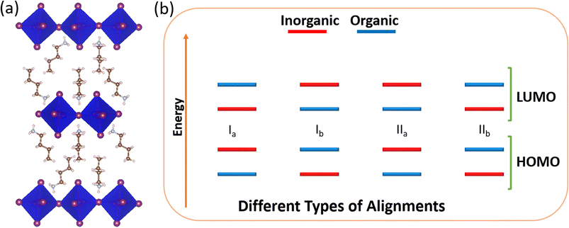Scheme 1 Schematic diagram of (a) a typical 2D hybrid perovskite structure and (b) different types of intramolecular band alignments in a 2D perovskite.

In type I_a, charge carriers are localised in the inorganic component having the possibility of inter-band excitonic transition, whereas in type I_b, carriers are localised in the organic component possessing a probability of π–π* transition. As a result, these types of materials are appropriate for lasers and light-emitting devices. On the other hand, in the case of type II materials, the carriers are separated into two different units, allowing longer carrier lifetime and are thus suitable for photovoltaic applications.^12–16

In this regard, Blum and co-workers have shown a direction to fine-tune the range of 2D perovskite materials targeting a particular electronic property through the quantum well aspect.¹⁷ Lu et al. have also shown how a spin–orbit coupling in metal halide and HOMO–LUMO energies of the organic cation control the intramolecular band alignments in these materials.¹⁸ Du and co-workers have demonstrated the role of polycyclic amines in tuning the band alignments of 2D hybrid perovskites.¹⁹ In our recent first principle-based study, we have shown that heterocyclic ring pyrilium and thiopyrilium-based spacer cations can directly contribute to band edges of the 2D hybrid perovskite materials.²⁰ Finding out the best material for a selective application from this wide availability is a difficult job by studying every individual material experimentally or computationally. Therefore, it is crucial that we develop a model that can predict the electronic properties of the system from its chemical composition so that we can identify the material of our desired properties easily.

In recent years, machine learning (ML) has played an important role in scientific research areas. Wang and co-workers have applied ML algorithms to discover stable lead-free hybrid perovskite.²¹ Castelli and co-workers have used it to predict the band gap of hybrid metal halide perovskites.²² Liang et al. have predicted the band gap of 2D hybrid perovskites using ML, whereas Wu and co-workers have developed an ML model to predict the formability of the low dimensional hybrid perovskites and classified them into 2D forming and Non 2D forming cases.^23,24 However, prediction of the electronic structure of the 2D hybrid perovskite materials is still unexplored. In this aspect, classification of these materials based on their electronic structures would be much appreciated and beneficial for the perovskite research community.

In the present work, we have, for the first time, classified the 2D halide perovskites into type I and type II band alignment quantum wells. Using the same dataset, we have further attempted to classify them into I_a, I_b, II_a, and II_b using a multiclass classification approach. We have also tried to classify type I and type II materials to their corresponding class I_a–I_b and II_a–II_b separately, considering individual datasets of type I and type II, respectively. For this purpose, we have utilised the physical as well as chemical properties of organic and inorganic units as features. Further, from feature coefficient analysis, we are able to find out the feature-output relations and give insights on the contribution of the features towards the output. In Scheme 2, we have picturised the flowchart of our work. Classification of 2D halide perovskites to their different band alignment types can help us in selecting the suitable material with desired features for their applications.

Scheme 2 Scheme of machine learning workflow for the current study.

The primary requirement of ML-based work is model training. A total of 103 2D perovskite materials have been considered, and their band alignment types were detected by performing density functional theory (DFT) calculations as well as from available theoretical reports. In the considered perovskite set, Pb and Sn are present as metal atoms, whereas Cl, Br and I are present as halogen with 80 different ammonium spacer cations (Fig. S1†).

Here, we have attempted to classify the considered perovskite materials based on their intramolecular band alignment types. In order to perform that, we have employed different molecular features of the perovskite material components as input. First, various ML algorithms were trained with these input features and their corresponding class as output. Afterwards, optimization of the hyperparameters of each of the considered models was performed, followed by selecting the best predictive model based on their classification accuracy. Finally, we have validated the predictability of the model by applying it to a few newly designed materials unknown to the trained model.

In this study, we have denoted the classification of the perovskite materials as output Y. 84 materials are collected from the 2D perovskite database developed by Tarasov and co-workers.²⁵ After performing single-point calculations on those crystal structures at the hybrid functional (HSE06) along with spin–orbit coupling (SOC) level (Text S1†), we have plotted the projected density of states (pDOS). Other 19 materials and their corresponding pDOS plots were obtained from the literature review.^19,20,26,27 Analysing the pDOS plots (Fig. S2†), we have identified their band alignment types and employed those as targets for the classification. In Fig. 1, we have demonstrated the band alignment types of 30 selected perovskites containing all four types of alignments.

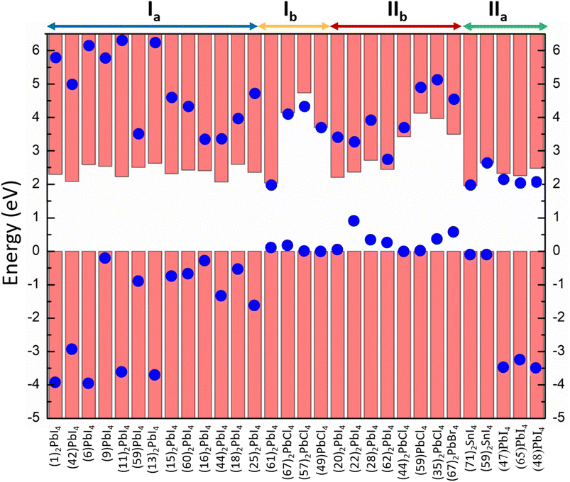Fig. 1 Band alignment types of 30 selected perovskites containing all four types of alignments. The structure of the numbered cation is listed in Fig. S1.†

Feature selection is one of the most important parts of ML-based studies, as simple and vital features may lead to a superior predictive model to predict the output accurately. For the inorganic units, we have considered the electronegativities of metal and halogen atoms along with the HOMO and LUMO energies of the MX₆ octahedral unit as features. To obtain this, we have taken a single MX₆ unit from the optimized methylammonium metal halide unit cell with four methyl ammonium cations (Fig. S3†) to make them neutral and performed single point calculation with the HSE06 + SOC method (Text S1†).^28–31 For the organic cations, we have calculated the HOMO and LUMO energies and utilized them as features. These calculations have been done in Gaussian 09 software.^32–40 To obtain some physicochemical properties of the ammonium cations, we have also considered some molecular descriptors. In general, target properties often depend on molecular descriptors, as physical and chemical properties are directly correlated with those parameters in many cases. Here, target property, i.e., types of band alignments, can be represented as a function of several molecular descriptors. These input descriptors can be transformed into useful chemical information through a mathematical procedure using the described function with respect to the target. These molecular descriptors contain not only experimental properties, such as molar refractivity, dipole moment, polarizability, and, in general, physicochemical properties, but also include theoretical molecular descriptors derived from symbolic representations, such as hydrogen bond-donor and acceptor count, topological polar surface area, vdW volume, vdW surface area etc. The details of the feature extraction and the list of the selected features are provided in ESI (Table S1 and Text S2†).

Data training is the key process of any ML project. Using the considered data set, we have performed model selection through hyperparameter tuning on different classifiers available in the open source scikit-learn package.⁴¹ Six such different classifiers (Text S3†), starting from simplest Logistic Regression, Ridge Classifier to complex models like Support Vector Machine, K-Nearest Neighbour, Bagging Classifier, and Random Forest Classifier, were selected for the model training process. After tuning of all the considered models with respect to their various hyperparameters, we obtained the best fitted model with its optimized hyperparameters. Next, to be assured about the stability of the models, we have used RepeatedStratified 5-fold cross-validation (Text S4†) and calculated the cross-validation accuracy of each of the considered models.⁴¹ Moreover, we have again divided the total data into a training set (∼70%) and test set (∼30%), keeping their ratio fixed for type I and type II data in both training and test sets and predicted for the test set using the model trained by the training set. In Table 1, we have tabulated best fitted model hyperparameters for all the considered ML models along with their test and cross-validation accuracy scores. The parameters other than hyperparameters related to the considered models are automatically estimated during the training process.

Table 1 Optimized hyperparameters and accuracy scores of considered ML algorithms

Classification algorithms	Optimized hyperparameters	Cross validation (average accuracy)	Test accuracy
Logistic regression	C: 0.01, penalty: l2, solver: lbfgs, tol: 1e^−4	0.83	0.86
Ridge classifier	Alpha: 0.8, solver: ‘auto’, tol: 1e^−4	0.83	0.79
Support vector machine	C = 50, kernel = rbf, degree = 3, gamma = ‘scale’, coef0 = 0.0, max_iter = −1	0.83	0.90
K nearest neighbor	Metric: manhattan, n_neighbors: 7, weights: uniform, algorithm: ‘auto’, leaf_size: 30, p: 2	0.82	0.86
Random forest classifier	Criterion: “gini”, max_features: log 2, n_estimators: 10, min_samples_leaf: 1, min_samples_leaf: 2	0.84	0.86
Bagging classifier (random forest as the base classifier)	n_estimators: 100, min_samples: 1, max_features: 1	0.84	0.93

---

The best cross-validation as well as test accuracy scores of 0.84 and 0.93, respectively, were achieved with the bagging classifier. Other algorithms also come up with nearly similar cross-validation accuracy scores in the range of 0.82 to 0.84 and similar test accuracy scores ranging from 0.79 to 0.93. Interestingly, the simplest algorithm logistic regression also results in a good cross-validation accuracy score (0.83) as well as a test accuracy score (0.86). We found out that the logistic regression model fails for four systems, which is mainly due to the strong overlap of inorganic and organic units at the band edges (Table S2†). This implies that those wrong predictions are not solely due to the wrong training of the model; rather, there is a hindrance in distinguishability due to the overlap of two different units at band edges. Hence, we can go ahead with logistic regression for our further analysis due to its simplicity, interpretability, as well as good predictability to retain the generalizability and transferability of the proposed model. Although we have achieved better accuracy with the bagging classifier, due to the complexity of these models, we did not move forward with this. Instead, we focused mainly on the transparency of the algorithm.

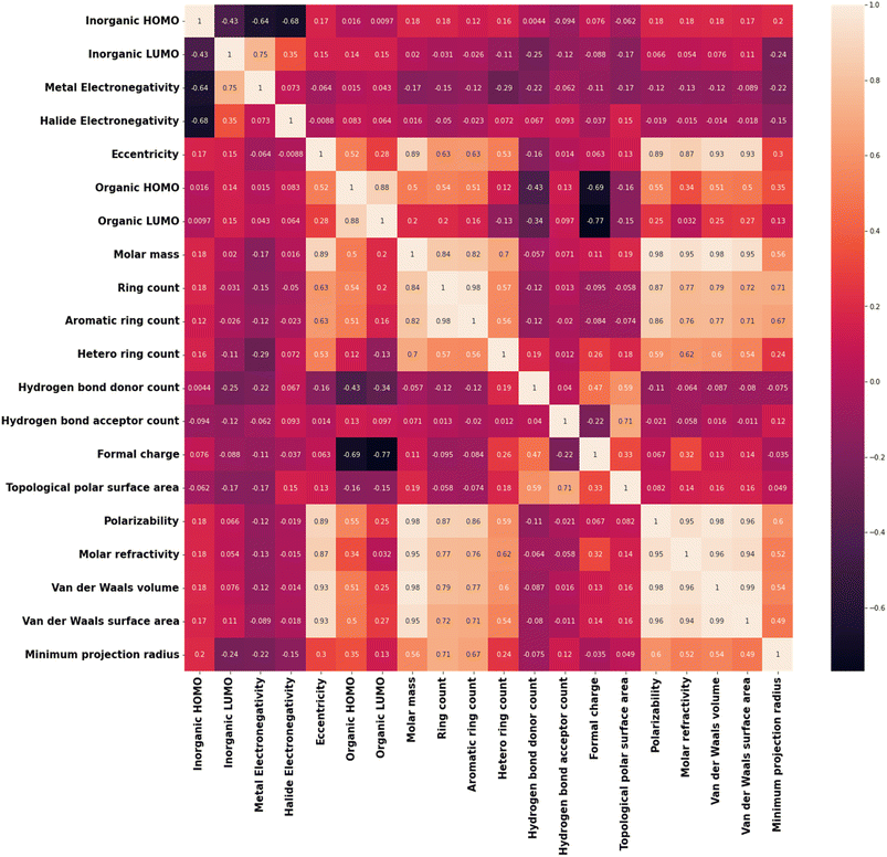
Apart from this, realizing the feature output relationship is important for advancing the ML analysis. For example, many of the selected features are highly correlated to each other. Among our considered features, polarizability and molar refractivity are highly correlated, whereas molar mass is correlated with vdW volume, vdW surface area, polarizability, and more. The formal charge of the cation is correlated with the HOMO and LUMO energies of the cation. There is a strong correlation between the HOMO and LUMO energies of the inorganic unit (metal halide octahedra) and the electronegativities of metal and halide. Reduction of these features (i.e., dimensionality) would not harm the accuracy of the model but rather will make the model simpler. In this regard, we have calculated the Pearson correlation coefficients (PCCs) and presented the plot in Fig. 2.⁴² Again, correlated features can also be helpful in many cases. In this regard, considering the logistic regression algorithm, we have analysed the model accuracy by deleting the correlated features one by one and observed similar results with only nine features (Table 2).

Fig. 2 Correlation matrix of the selected features with Pearson correlation coefficients.

Table 2 Finally selected 9 features upon feature engineering

Serial no.	Selected features
1	Organic HOMO (OH)
2	Organic LUMO (OL)
3	Inorganic HOMO (IH)
4	Inorganic LUMO (IL)
5	Metal electronegativity (ME)
6	Halogen electronegativity (HE)
7	Hydrogen bond-donor count (HBDC)
8	Hydrogen bond-acceptor count (HBAC)
9	Polarizability (α)

---

Also, we have used the recursive feature elimination method for selecting the proper combination of features to improve the accuracy and obtained the plot for accuracy score vs. number of features (Fig. S4†). Interestingly, the accuracy score increased slightly (0.89) with twelve features compared to the previous accuracy score (0.86) with nine features. Therefore, based on the recursive feature elimination method, important features such as the LUMO energy of the inorganic unit and electronegativity of the metal need to be excluded. On the other hand, highly correlated features such as polarizability-molar refractivity (PCC: 0.95) and polarizability-van der Waals surface area (PCC: 0.96) need to be included. This happens because this method ranked the features according to their weightage or coefficient evaluated by a certain algorithm. However, we know that HOMO and LUMO energies of the organic and inorganic components play important roles in tuning the band alignments. So, instead of relying only on the feature selection method, we focused on our scientific understanding of the feature output relation and continued with nine features.

Notably, these nine features are sufficient to classify the materials with good accuracy (90%). We could reach good accuracy in the classification prediction as there is a strong inherent relation between the band alignment of 2D perovskites and their molecular and elemental features. We have noticed that the valence band edge of the material is mainly constituted of the organic cation if the HOMO of the organic cation is less stabilised. On the other hand, the conduction band edge of the material is constituted of organic spacer cation when we have a stabilised LUMO orbital of the organic cation. This is very much consistent with the previous reports.^18,19,27,43 For example, Shu and co-workers have demonstrated that the frontier molecular orbitals of organic spacer cations as well as inorganic layers can be the key factors in determining their band alignment types.⁴³ Similarly, Lu and co-workers and Du and co-workers have shown the possibility of four types of intramolecular band alignment quantum wells by changing the different types of organic spacer cations.^18,19 Scanlon and co-workers have also shown that metal halide variations keeping the spacer cation fixed can also lead to different band compositions.²⁷ Also, other molecular features, such as hydrogen bond-donor/acceptor count, can be an important factor in predicting band alignment types. Molecular features such as the polarizability of the organic spacer cation significantly influence the geometry as well as orbital energies of the cation, which have also been shown by Yang and co-workers, and we have also studied this in detail theoretically in our previous work.^20,44 Hence, there is a good relation between the molecular features and band alignment types. We have also observed there can be a good relation between the band alignment types and elemental features of the organic/inorganic unit. For example, as we go down the halogen group, the HOMO orbital energy increases and therefore dominates the valence band edge of the material. Therefore, for our future analysis, we will use these features only.

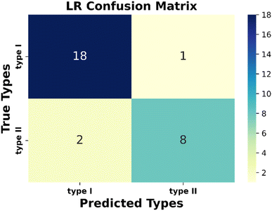
Next, the evaluation of the considered models has been performed. Performance metrices are very useful for evaluating the operation capability of the considered model and gaining insights into the dataset containing diverse data points. There are some metrices that evaluate the quality of the classification algorithm performance. Here, we have used classification accuracy, F1 score, precision, and recall to justify the model. All these metrices can be calculated from the confusion matrix (Fig. S5 and Text S5†). From the obtained confusion matrix (Fig. 3) with the considered test dataset, we have observed that type I and type II materials have been correctly predicted for 18 and 8 instances, respectively. Interestingly, only once type I material is predicted as type II, whereas type II as type I twice. So, from this observation, we can conclude that our proposed model can be applicable to the other unexplored materials with satisfactory accuracy.

Fig. 3 Confusion matrix for the type I and type II classification of considered 2D perovskite.

Again, in Table 3, we have tabulated the calculated values of the classification metrices. For the positive class (type I), we got precision, recall, and f1-score as 0.90, 0.95 and 0.92, respectively. Whereas for the negative class, these metrices are 0.89, 0.80, and 0.84, respectively. So, the model is ready to implement on the unknown datasets.

Table 3 Classification parameters of binary classification of type I and type II

Class	Precision	Recall	F1-score
Type I	0.90	0.95	0.92
Type II	0.89	0.80	0.84

---

In continuation, we performed binary classification of type I and type II materials separately and observed an improved accuracy score. For the binary classification of type I materials into I_a–I_b, with 71 pieces of data and type II materials into II_a–II_b with 32 pieces of data, we have found up to 93% and 98% average cross-validation accuracy, respectively (Table S3†). We have further tried to classify the materials into their four distinct classes: I_a, I_b, II_a, and II_b. For that, we have performed multiclass classification with logistic regression using one vs. rest method and achieved 76% average cross-validation accuracy (Table S3†). In this case, due to an imbalanced dataset, which means an unequal ratio of four classes, we have observed low accuracy. Further, we have separated all three datasets to train-test sets and performed classification to obtain classification metrices and confusion matrix. In ESI (Text S6, Tables S3–S6, and Fig. S6–S8†), we have presented the model details along with the classification metrices and confusion matrices. In the case of II_a–II_b binary classification, we have a nearly equal ratio of two classes. From the tabulated classification metrices (Table S5) and confusion matrix (Fig. S7†), we can notice very good classification results for the II_a–II_b binary classification. This observation is entirely due to the good ratio of two classes in the dataset. Although the overall result is good for I_a–I_b classification, it can be easily understood from the confusion matrix (Fig. S3†) that the training of I_b is not proper due to its smaller number in the dataset. So, although we can get a reasonably good confusion matrix in the case of type I–II classification, we believe that the confusion matrix results in the prediction of all the individual classes (I_a, I_b, II_a, II_b) with the same model can be improved if we can make a balance in training data for all the individual classes to be predicted. Unfortunately, till date, reported type I_b materials are much less compared to the type I_a materials.

We have proposed 17 new perovskite materials to validate our model. We have designed these 17 new materials and calculated their properties using DFT. Accounting for the good predictability of the logistic regression algorithm, we have applied this algorithm with the optimized hyperparameters to the newly modelled dataset and observed an accuracy score of 0.88. Our model fails to predict the cases when there is a strong overlap of organic and inorganic components in the band edges. Hence, our model is capable enough to identify type I and type II materials properly. The materials with their predicted and actual class have been shown in ESI (Table S7†). Among the materials we have designed, four are type II band alignment quantum wells. Although finding type II material is a challenging task, we successfully found four such materials, which can be useful for future applications.

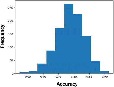
Again, we have confirmed the performances of the model by calculating the confidence interval using 1000 bootstrap iterations. From these bootstrap iterations, we have found a 95% likelihood of classification accuracy between 69% and 87%. However, it can be noticed from Fig. 4 that the major portions of the iterations are shifted towards an accuracy score greater than 0.75. It certainly indicates the good predictive capability as well as stability of the model.

Fig. 4 Frequency vs. accuracy plot.

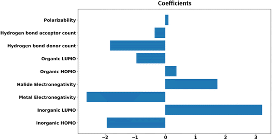
For the generalizability and transferability of a model, proper formulation from chemical understanding and model analysis is necessary. We have calculated the feature contribution coefficients of the selected nine features (Fig. 5). Implementing these values in logistic regression, we can formulate a probability equation to predict the band alignment type of a 2D perovskite easily.

Fig. 5 Feature contributions of the finally selected nine features towards output Y.

According to the logistic regression algorithm, the probability of a positive label (P_typeI(x_i)) can be represented as,

where m is the feature contribution coefficient, and x is the value of the feature.

From the implemented algorithm used for our considered dataset, the derived equation can be expressed as

From the feature contribution coefficients, we can obtain the mathematical form of the trained ML model and provide chemical insights. Here, from Fig. 5, we can see that some features have positive contributions, whereas some have negative contributions. Since our calculated orbital energies (HOMO and LUMO of organic and inorganic units) are with negative signs, they will give an overall reverse contribution to the classification. That means the positively contributing features are contributing to the negative classes and vice versa.

Inorganic–organic HOMO/LUMO coefficients are contributing in the following order: inorganic LUMO > inorganic HOMO > organic LUMO > organic HOMO. Inorganic HOMO and organic LUMO have negative contribution coefficients. However, the type of band alignment depends on the relative position of these energy levels, and they are highly interdependent with respect to other features as well. Moreover, the inorganic HOMO–LUMO values were considered as fixed values for a particular inorganic unit, but this can be changed in the presence of different organic spacer cations. Hence, it is difficult to explain in the light of physicochemical perspective.

The electronegativity of metal and halide contributes to the negative and positive classes, respectively. More electronegative halide will make lower energetic molecular orbitals. A material having highly stable organic LUMO can make the conduction band with organic dominance, and stability of the inorganic HOMO might help to form a type I band alignment with organic–organic combination.

Polarizability is also contributing positively, as per the feature analysis. This indicates that the more polarisable organic cation will tend to form perovskite with type I band alignment. As we know, highly conjugated organic cations are electron-rich and thus more polarisable in nature, and the previous reports demonstrate that such polarisable molecules have a small HOMO–LUMO gap.^45,46 Hence, we can tune the valence/conduction band edges of the material with polarisable organic cation.

Hydrogen bond-donor and -acceptor count has a negative contribution towards the output that increases the possibility of type II band alignment perovskite material. Hydrogen bond-donor count means hydrogens available for the formation of H-bonds with inorganic layer halides. Strong H-bonding with the halides will decrease the overlap between halogen and metal, which in turn will increase the HOMO and LUMO gap between the inorganic unit. Hydrogen bond-acceptor count is responsible for intramolecular H-bonding, which makes the spacer cation rigid and reduces its interaction with the metal halide layer. Smaller interaction with the organic unit will keep the inorganic layer undistorted, and the overlap between the metal and halide orbitals will be larger, which will decrease the HOMO LUMO gap of the inorganic unit.⁴⁴ Thus, the probability of type II band alignment perovskite increases with high hydrogen bond-donor and -acceptor nature of the organic unit.

We have analysed the effects of the important features those are mainly contributing to the classification. All these features have some distinct contribution to making the material type I or type II band alignment quantum well. But these features are interdependent with each other. That means no single feature can itself make a material to be in a positive class or negative class, such that one feature is providing a significant contribution to put a perovskite in the positive class, but the material will be in the positive class depending on the performance of the other features.

In conclusion, we have successfully classified 2D hybrid perovskites into type I and type II band alignment quantum wells and extracted the strategy to obtain a specific electronic property as well. An excellent classification accuracy score of 0.90 has been found with the simplest logistic regression algorithm using nine important features. Moreover, utilising feature contribution coefficients, HOMO and LUMO of the inorganic as well as organic units and metal-halogen electronegativities are found to be the most contributing features. Additionally, we have validated our model with unknown 17 hybrid perovskite materials and found a reasonably good accuracy score (0.88). Our model has misidentified only two type II material as type I, which has merged contribution at the band edge from both organic and inorganic parts. Apart from this, we have tried to classify all four band alignment types (type I_a, I_b, II_a, II_b) using multiclass classification and classified type I and II towards I_a–I_b and II_a–II_b band alignment types. Finally, we have established an equation for predicting the probability of finding band alignment types based on our calculated feature contribution coefficients. Overall, our proposed strategy opens a new direction towards utilizing ML for screening 2D perovskites for various applications.

Conflicts of interest

There are no conflicts to declare.

Acknowledgements

We thank IIT Indore for the lab and computing facilities. This work is supported by DST-SERB [Project Number: CRG/2018/001131 and CRG/2022/000836] and CSIR [Project Number: 01(3046)/21/EMR-II]. E. M., D. R., and S. S. M. thank MHRD and CSIR for the research fellowships.

References

1. A. Kojima, K. Teshima, Y. Shirai and T. Miyasaka, J. Am. Chem. Soc., 2009, 131, 6050–6051.
2. M. M. Lee, J. Teuscher, T. Miyasaka, T. N. Murakami and H. J. Snaith, Science, 2012, 338, 643–647.
3. J. Burschka, N. Pellet, S.-J. Moon, R. Humphry-Baker, P. Gao, M. K. Nazeeruddin and M. Grätzel, Nature, 2013, 499, 316.
4. A. K. Jena, A. Kulkarni and T. Miyasaka, Chem. Rev., 2019, 119, 3036–3103.
5. J. M. Frost, K. T. Butler, F. Brivio, C. H. Hendon, M. van Schilfgaarde and A. Walsh, Nano Lett., 2014, 14, 2584–2590.
6. Y. Zhao and K. Zhu, Chem. Commun., 2014, 50, 1605–1607.
7. I. C. Smith, E. T. Hoke, D. Solis-Ibarra, M. D. McGehee and H. I. Karunadasa, Angew. Chem., Int. Ed., 2014, 53, 11232–11235.
8. C. C. Stoumpos, D. H. Cao, D. J. Clark, J. Young, J. M. Rondinelli, J. I. Jang, J. T. Hupp and M. G. Kanatzidis, Chem. Mater., 2016, 28, 2852–2867.
9. L. N. Quan, M. Yuan, R. Comin, O. Voznyy, E. M. Beauregard, S. Hoogland, A. Buin, A. R. Kirmani, K. Zhao, A. Amassian, D. H. Kim and E. H. Sargent, J. Am. Chem. Soc., 2016, 138, 2649–2655.
10. C. Katan, N. Mercier and J. Even, Chem. Rev., 2019, 119, 3140–3192.
11. D. Sapori, M. Kepenekian, L. Pedesseau, C. Katan and J. Even, Nanoscale, 2016, 8, 6369–6378.
12. K. Wei, T. Jiang, Z. Xu, J. Zhou, J. You, Y. Tang, H. Li, R. Chen, X. Zheng and S. Wang, et al. , Laser Photonics Rev., 2018, 12, 1800128.
13. K. Chondroudis and D. B. Mitzi, Chem. Mater., 1999, 11, 3028–3030.
14. D. Liang, Y. Peng, Y. Fu, M. J. Shearer, J. Zhang, J. Zhai, Y. Zhang, R. J. Hamers, T. L. Andrew and S. Jin, ACS Nano, 2016, 10, 6897–6904.
15. J. Yin, H. Li, D. Cortecchia, C. Soci and J.-L. Bredas, ACS Energy Lett., 2017, 2, 417–423.
16. J. C. Blancon, A. V. Stier, H. Tsai, W. Nie, C. C. Stoumpos, B. Traore, L. Pedesseau, M. Kepenekian, F. Katsutani and G. T. Noe, et al. , Nat. Commun., 2018, 9, 2254.
17. C. Liu, W. Huhn, K.-Z. Du, A. Vazquez-Mayagoitia, D. Dirkes, W. You, Y. Kanai, D. B. Mitzi and V. Blum, Phys. Rev. Lett., 2018, 121, 146401.
18. L. Zhang, X. Zhang and G. Lu, J. Phys. Chem. Lett., 2020, 11, 6982–6989.
19. D. Han, S. Chen and M.-H. Du, J. Phys. Chem. Lett., 2021, 12, 9754−9760.
20. E. Mahal, S. C. Mandal and B. Pathak, J. Phys. Chem. C, 2022, 126, 9937–9947.
21. S. Lu, Q. Zhou and Y. Ouyang, et al. , Nat. Commun., 2018, 9, 3405.
22. W. A. Saidi, W. Shadid and I. E. Castelli, npj Comput. Mater., 2020, 6, 36.
23. Z. Wan, Q. D. Wang, D. Liu and J. Liang, New J. Chem., 2021, 45, 9427–9433.
24. R. Lyu, C. E. Moore, T. Liu, Y. Yu and Y. Wu, J. Am. Chem. Soc., 2021, 143, 12766−–12776.
25. E. I. Marchenko, S. A. Fateev, A. A. Petrov, V. V. Korolev, A. Mitrofanov, A. V. Petrov, E. A. Goodilin and A. B. Tarasov, Chem. Mater., 2020, 32, 7383–7388.
26. J. Xue, R. Wang, X. Chen, C. Yao, X. Jin, K.-L. Wang, W. Huang, T. Huang, Y. Zhao and Y. Zhai, et al. , Science, 2021, 371, 636–640.
27. Z. Wang, A. M. Ganose, C. Niu and D. O. Scanlon, J. Mater. Chem. C, 2019, 7, 5139–5147.
28. P. Giannozzi, S. Baroni, N. Bonini, M. Calandra, R. Car, C. Cavazzoni, D. Ceresoli, G. L. Chiarotti, M. Cococcioni, I. Dabo, A. Dal Corso, S. de Gironcoli, S. Fabris, G. Fratesi, R. Gebauer, U. Gerstmann, C. Gougoussis, A. Kokalj, M. Lazzeri, L. Martin-Samos, N. Marzari, F. Mauri, R. Mazzarello, S. Paolini, A. Pasquarello, L. Paulatto, C. Sbraccia, S. Scandolo, G. Sclauzero, A. P. Seitsonen, A. Smogunov, P. Umari and R. M. Wentzcovitch, J. Phys.: Condens. Matter, 2009, 21, 395502.
29. J. Heyd, G. E. Scuseria and M. Ernzerhof, J. Chem. Phys., 2003, 118, 8207–8215.
30. M.-H. Du, J. Phys. Chem. Lett., 2015, 6, 1461–1466.
31. H. J. Monkhorst and J. D. Pack, Phys. Rev. B: Solid State, 1976, 13, 5188–5192.
32. J. Frisch, et al., Gaussian Revision D.01, Gaussian, Inc., Wallingford CT, 2013.
33. W. J. Hehre, K. Ditchfield and J. A. Pople, J. Chem. Phys., 1972, 56, 2257–2261.
34. P. C. Hariharan and J. A. Pople, Theor. Chim. Acta, 1973, 28, 213–222.
35. R. Krishnan, J. S. Binkley, R. Seeger and J. A. Pople, J. Chem. Phys., 1980, 72, 650–654.
36. A. D. Becke, Phys. Rev. A, 1988, 38, 3098–3100.
37. A. D. Becke, J. Chem. Phys., 1993, 98, 5648–5652.
38. A. D. Becke, J. Chem. Phys., 1997, 107, 8554–8560.
39. A. D. Becke, J. Chem. Phys., 1993, 98, 1372–1377.
40. C. Lee, W. Yang and R. G. Parr, Phys. Rev. B: Condens. Matter Mater. Phys., 1988, 37, 785–789.
41. F. Pedregosa, G. Varoquaux, A. Gramfort, V. Michel, B. Thirion, O. Grisel, M. Blondel, P. Prettenhofer, R. Weiss, V. Dubourg, J. Vanderplas, A. Passos and D. Cournapeau, J. Mach. Learn. Res., 2011, 12, 2825–2830.
42. R. Tibshirani, J. R. Stat. Soc. Ser. B, 1996, 58, 267–288.
43. Y. Yao, D. Cao, J. Yan, M. Zhang, X. Chen and H. Shu, J. Phys. Chem. C, 2022, 126, 8408–8416.
44. C. Ni, Y. Huang, T. Zeng, D. Chen, H. Chen, M. Wei, A. Johnston, A. H. Proppe, Z. Ning and E. H. Sargent, et al. , Angew. Chem., Int. Ed., 2020, 59, 13977–13983.
45. K. Kamada, M. Ueda, H. Nagao, K. Tawa, T. Sugino, Y. Shmizu and K. Ohta, J. Phys. Chem. A, 2000, 104, 4723–4734.
46. S. R. Jezowski, R. Baer, S. Monaco, C. A. Mora-Perez and B. Schatschneider, Phys. Chem. Chem. Phys., 2017, 19, 4093–4103.

---

Footnote

† Electronic supplementary information (ESI) available: Figures of the considered ammonium spacer cations, details of the computational methods, list of selected features, details of machine learning algorithm and cross-validation method, details of classification metrices and confusion matrix, test dataset, validation dataset, and total dataset of 103 materials. See DOI: https://doi.org/10.1039/d3ta05186b

---