DPD simulations of anionic surfactant micelles: a critical role for polarisable water models

Abstract

We investigate the effects of polarisable water models in dissipative particle dynamics (DPD) simulations, focussing on the influence these models have on the aggregation behaviour of sodium dodecyl sulfate solutions. Studies in the literature commonly report that DPD approaches underpredict the micellar aggregation number of ionic surfactants compared to experimental values. One of the proposed reasons for this discrepancy is that existing water models are insufficient to accurately model micellar solutions, as they fail to account for structural changes in water close to micellar surfaces. We show that polarisable DPD water models lead to more realistic counterion behaviour in micellar solutions, including the degree of counterion disassociation. These water models can also accurately reproduce changes in the dielectric constant of surfactant solutions as a function of concentration. We find evidence that polarisable water leads to the formation of more stable micelles at higher aggregation numbers. However, we also show that the choice of water model is not responsible for the underestimated aggregation numbers observed in DPD simulations. This finding addresses a key question in the literature surrounding the importance of water models in DPD simulations of ionic micellar solutions.

---

1 Introduction

Since its inception, DPD has found widespread use in the simulation of complex and computationally demanding soft matter systems, including polymer and surfactant solutions.^1–12 DPD allows for significantly faster equilibration time than traditional molecular dynamics (MD) approaches, making it particularly applicable to systems where spontaneous aggregation occurs: such as micellar solutions,^1–6 lyotropic liquid crystals,^6,12–15 and chromonic mesophases^16,17 or systems where complex molecular self-organisation occurs.^18–20 In this paper, we study the aggregation behaviour of the well-known anionic surfactant sodium dodecyl sulfate (SDS) using DPD, and address one of the key weaknesses of standard DPD approaches: the inability to predict the correct dielectric behaviour of aqueous solutions.

SDS has been the focus of many experimental studies across literature, due to its widespread use in commercial products, particularly in personal care products. Aqueous SDS solutions are arguably one of the most studied systems in surfactant research. This is particularly true of the micellar phase,^21–33 although higher concentration liquid phases have also been extensively characterised.^34–36 Much of the literature dedicated to micellar solutions has focused on determining the shape, size, and structure of micelles, as well as looking at the impact of variables such as salt,^{23–25,27–29} temperature,^29–31 and concentration.^{26–29,31–33} Other research has looked at the impact of mixing surfactants with other components such as other surfactants,^22,24,26,30 to understand the changes this may produce in micellar properties. However, despite the abundance of SDS studies in literature, experimental data can often be difficult to interpret as studies can often conflict with each other. In particular, different experimental approaches usually lead to different conclusions surrounding the size and shape of SDS micelles, complicating our understanding of these systems.

Due to the difficulties associated with interpreting experimental data, as highlighted above, SDS has also been the focus of numerous existing theoretical and modelling studies. Such studies can help provide insight where experiments may struggle. Theoretical thermodynamic models have been used to predict the properties of micelle solutions using the free energy of formation of an aggregate in solution.^37–40 These models can be used to predict the critical micelle concentration (CMC), and the average expected size and shape of aggregates. Simulation studies range from detailed all-atom MD approaches,^41–45 to those using coarse-grained approaches such as DPD.^1–5 Here, MD simulations are typically limited to studying very small systems and are often prohibitively computationally expensive for studying systems consisting of multiple micelles, or for studying the aggregation process itself. This makes it desirable to develop accurate DPD modelling techniques to allow one to study far larger systems at longer time scales using a simulation approach. Other approaches to predicting surfactant properties include field-based approaches such as self-consistent field theory.^46–48

There are several existing studies using DPD to study SDS solutions. However, most of these studies have taken the traditional DPD approach:^4,5i.e., simulations are carried out with an uncharged model in which explicit electrostatic interactions are not included. The first attempt to model SDS with explicit electrostatics was presented by Mao et al.,² which was followed a few years later by Anderson et al.³ Both models were found to significantly underestimate the aggregation number in comparison to experimental values. Potential reasons proposed by the authors for this discrepancy include equilibration issues,³ inadequate calculation of the short-range repulsion parameters,^2,3 and the treatment of charged particles.²

One interesting suggestion made by both sets of authors,^2,3 is that underpredicted aggregation numbers may result from the typical treatment of water in DPD. Specifically, coarse-grained simulation techniques such as DPD are typically performed using a constant dielectric constant across the simulation box. This approach may be inadequate for taking into account the structural changes of water near charged surfaces, such as those seen with a charged micelle.^49–51 We propose that this may result in the degree of counterion dissociation being artificially inflated, and causing smaller micelle sizes. A change in counterion dissociation is also highly likely to influence micelle-micelle interactions. In this article, we aim to address this suggestion by making use of a polarisable water model.

Very few polarisable water models for DPD have been proposed in the existing literature. Existing models are those presented by Peter and Pivkin,⁵² Peter et al.,⁵³ Vaiwala et al.⁵⁴ and, most recently, Chiacchiera et al.⁵⁵ In this paper, we begin by presenting a study of these existing models for the purpose of applying them to micellar solutions. However, we show that the Peter and Pivkin⁵² and Peter et al.⁵³ models do not reproduce the dielectric constants that they claim to, and instead produce dielectric constant values for water which are much lower than the experimental values. Therefore, we base our polarisable water model on the work of Vaiwala et al.⁵⁴ To the best of our knowledge, this is the first attempt at modelling ionic micelles using DPD with a polarisable water model.

2 Dissipative particle dynamics

2.1 Overview of forces

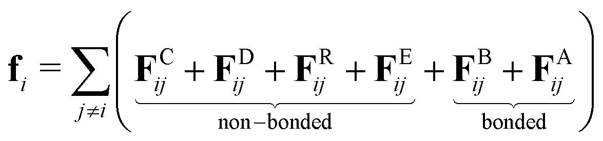
DPD is a coarse-grained simulation method in which groups of atoms are represented by soft ‘beads’. The relative softness of the interbead forces allows for long time steps, enhanced diffusion, and faster equilibration times in comparison to both atomistic and coarse-grained molecular dynamics.

The total force acting on bead i can be written as a sum of contributing forces from bonded and non-bonded components:

where F_ij are the forces acting on bead i by bead j. The non-bonded contribution is made up of the conservative F^C_ij, dissipative F^D_ij, random F^R_ij and electrostatic F^E_ij forces. These forces act within a defined cut-off range r_C (excluding the electrostatic force) and beyond this they are taken to be zero. This relatively short cut-off range contributes to the fast computational speed of the DPD method. The conservative force takes the formwhere 0 < a_ij which results in a repulsion between beads i and j since r_ij = r_i − r_j is the vector between beads i and j and unit vector r̂_ij = r_ij/|r_ij|. The dissipative and random forces are given by the following expressions

F^D_ij = −γω^D(r_ij)(r̂_ij·v_ij)r̂_ij, (3)

F^R_ij = σω^R(r_ij)ζ_ijr̂_ijΔt^−1/2, (4)

where ω^D and ω^R are weight functions that vanish when |r_ij| > r_C. γ is a friction coefficient and σ is the noise amplitude, v_ij = v_i − v_j is the velocity between beads i and j, Δt is the time step and ζ_ij(t) is a randomly fluctuating Gaussian variable with zero mean and unit variance. To satisfy the fluctuation-dissipation theorem,⁵⁶ the relationship between the weight functions has the requirement that

ω^D = [ω^R]² (5)

and the relationship between the amplitudes is

σ² = 2γk_BT, (6)

where k_B is the Boltzmann constant and T is the temperature. In this work, we set k_BT = 1 and set values for the constants σ = 3 and γ = 4.5. The form chosen for the weight functions isfor when |r_ij| < r_C, since it maintains simplicity. The bonding forces are calculated from bonding potentials U^B_ij and U^A_ij, where U^B_ij chemically bonds beads together, while U^A_ij defines a rigidity between molecules. These potentials take the formwhere l₀ is an equilibrium bond length and C is a constant defining the strength of the bond. θ_ijk is a bond angle between beads i, j and k, and θ₀ is an equilibrium bond. The constant D defines how strongly this rigidity is implemented. Note that we use a timestep of Δt = 0.01 for all of the simulations conducted in this work.

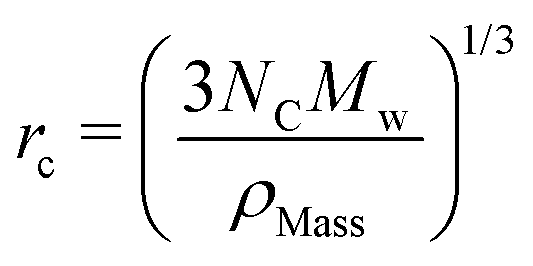
The r_C parameter serves as a means for converting DPD length scales into real units. A value for r_C is usually calculated by matching the density of water simulated to the density of water experimentally at room temperature. This is dependent on the choice of bead density ρ_D and the degree of coarse graining used for water N_C. We take the conventional choice of ρ_D = 3r_C⁻³, resulting in r_C being determined by the expression

where M_w is the mass of one water molecule and ρ_Mass is the experimental value of the density of water at room temperature ρ_Mass = 997 kg m⁻³. In this work, we make use of two different models for coarse-graining. Hence, the values calculated for r_c are given in Section 4 once the surfactant models have been introduced. All simulations described in this article are performed using the LAMMPS software package.⁵⁷

2.2 Electrostatics in DPD

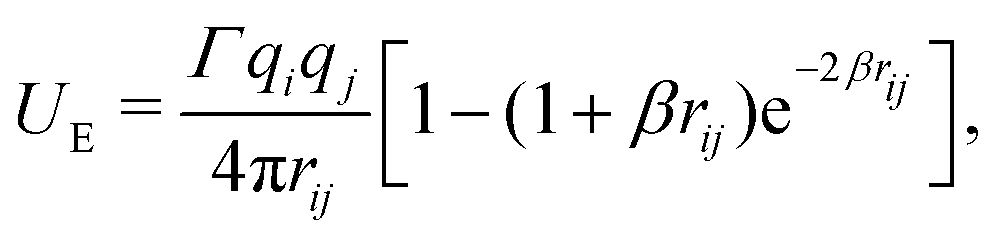
Electrostatics are implemented using smeared charges to avoid artificial ion pair formation. This has become the standard approach for DPD simulations.^2,3,54,58 Various forms of the smearing function have been proposed in the literature,⁵⁹ including a linear charge distribution, where the charge distribution ρ(r) is given aswhere R is the smearing distance and q is the charge. A popular alternative is to use the Slater-type smearing, where the charge distribution is given bywhere λ is the decay length of the charge. This charge distribution results in a relatively complex expression for the electrostatic potential:⁵⁹where q_i and q_j are the charges on two beads, Γ = e²/(k_BTε₀ε_sr_C) is a dimensionless electrostatic coupling parameter, β = 1/λ is the Slater parameter, ε₀ is the permittivity of free space and ε_s is the background relative permittivity. Therefore, typically a simplified form of the potential is usually used:which is also the form we choose to use in this work. Note that when standard (non-polarisable) water models are used, the relative permittivity of the solvent ε_r replaces ε_s in the definition of Γ, becoming the background permittivity. For simulations in which we use standard DPD water, we set ε_r ≈ 78.3. For polarisable water models, one can choose to set the background permittivity equivalent to that of a vacuum (ε_s = 1) or potentially of another material. For example, since we do not intend to consider the electrostatic interactions of the hydrophobic core of the micelles we simulate, one could set the background screening to a value which reflects a screening comparable to alkanes. This will be discussed in more detail in the following section.

We base our polarisable water model on the work of Vaiwala et al.,⁵⁴ who used a linear charge distribution function (with R = 1.6r_C, as suggested by Groot⁵⁸). However, the surfactant models we use were originally tested using the Slater-type charge density distribution. These parameterisations were calculated by Anderson et al.³ (using β = 0.929r_C, as suggested by González-Melchor et al.⁶⁰) and Mao et al.² (using β = 4r_C). The R = 1.6r_C and β = 0.929r_C choices for the linear and Slater smearing result in nearly identical electrostatic potentials, and in particular the Slater-type potential with β = 0.929r_C has been used extensively throughout the literature. Consequently, throughout this work, we chose to use the Slater-type potential with β = 0.929r_C. Noting that a slight variation of electrostatic treatment from the original Vaiwala et al. paper may result in very slight differences in results compared to those originally published.

3 Polarisable water model and calculating the dielectric constant

The polarisable water model used is based on the work of Vaiwala et al.⁵⁴ and is illustrated in Fig. 1. We note in passing the similarity of this model to the polarisable Martini model and variants^61–64 that are commonly used in coarse-grained models of biological^65,66 and soft-matter systems.⁶⁴ It is also noted that an interesting alternative is provided by a charged dimer model, such as discussed in the recent work of Chiacchiera.⁵⁵ In Fig. 1, water particles are treated as Drude oscillators with a central water bead (W) and two attached oppositely charged beads (D). The central bead represents multiple water molecules (2 or 4 waters in this work - see Section 4). It is important to note that beads that are directly bonded do not interact with each other (i.e. the central water bead and Drude beads do not interact with each other through space when they belong to the same particle). Drude beads (D) interact with the Drude beads of another particle via the dissipative, random and electrostatic forces, but do not interact via the conservative force. Central water beads (W) interact via all forces except the electrostatic force. These force interactions are summarised in Table 1.

Fig. 1 Model for polarisable water particles. Each particle is made up of a central water bead (W) attached to two charged Drude beads (D) possessing charges ±q.

Table 1 Summary of how beads interact with each other within water particles

	F ^C ij	F ^Dij	F ^R ij	F ^E ij	F ^B ij	F ^A ij
W–W	✓	✓	✓
W–D (intra)					✓	✓
W–D (inter)		✓	✓
D–D (intra)						✓
D–D (inter)		✓	✓	✓

---

The total mass of the water particle is m, where the central water bead has mass 2m/3 and each of the Drude beads has mass m/6. In practice, reduced units are used where the DPD particle mass m = 1. The bond between Drude beads and water beads is controlled by eqn (8), where the length of the bond is set as l₀ = 0.35r_C, and the strength is set by C = 512k_BT/r_C². The angle between the bonded beads (D–W–D angle) is controlled by eqn (9) where the equilibrium bond angle θ₀ = 0 and D = 1k_BT/rad². These parameter choices are based on the work of Vaiwala et al.⁵⁴ It is important to note that although the Drude beads do not interact within their own particle, we observe that there is no effect on the temperature control because of this. All beads are thermalized by collisions in the system, and we find no difference in the temperature of individual beads across the simulation.

The relative permittivity (dielectric constant) of the solvent ε_r is calculated using classical Fröhlich–Kirkwood theory,^67,68 using the fluctuations of the total dipole moment M

where T is the system's temperature and V is the volume. The total dipole moment is calculated as where q is the Drude charge, N_W is the number of water particles, and r_k⁺ and r_k⁻ are the positions of the positively and negatively charged Drude beads. Note that in the absence of an external field, we expect that 〈M〉² = 0.

Similarly to Vaiwala et al.,⁵⁴ we chose to set ε_s = 2. Since alkanes tend to possess a dielectric constant value ≈2,⁶⁹ this choice reasonably reproduces the dielectric screening of the micelle core. Therefore, to reproduce the correct relative permittivity for water, we aim for a target value of ε_r/ε_s = 78.3/2 ≈ 39.2.

Vaiwala et al.⁵⁴ base their water parameterisation on a mapping of four water molecules per DPD bead. The model is parameterised to reproduce the compressibility of water at room temperature and relative dielectric permittivity. The compressibility of the fluid is primarily influenced by the choice of a_WW. To reproduce the compressibility of water at room temperature, the conservative repulsion for water beads a_WW is typically defined as a_WW ≈ 25N_Ck_BT/r_C, where N_C is the degree of coarse graining. Using this relation, Vaiwala et al.⁵⁴ choose to set a_WW = 100.

The relative dielectric permittivity is largely influenced by the choice of Drude charge q and the equilibrium bond length l₀. In the following sections, we discuss surfactant parameterisations based on the use of different values of a_WW, and therefore we simulate using the same a_WW values that the surfactant parameterisations were based on. In theory, deviating from a_WW = 100 also influences the calculated dielectric constant (in addition to l₀ and q). However, we will show that the dielectric constant calculated is largely independent of a_WW.

4 Surfactant models

We apply the polarisable water model (discussed in the previous section) to solutions containing micelles formed by sodium dodecyl sulfate (SDS). We investigate the effect of the polarisable water on two different parameterisations of SDS. The first of these models was developed by Mao et al.,² which was also one of the first models of SDS in DPD to explicitly include electrostatic charges. The second of these models is that developed by Anderson et al.³ The coarse graining of SDS used in both of these parameterisation schemes is illustrated in Fig. 2.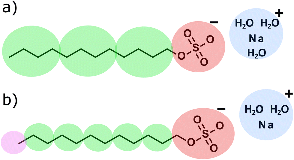

Fig. 2 Coarse-graining used in the (a) Mao et al.² and (b) Anderson et al.³ parameterisation schemes of SDS. Beads are coloured according to type.

In the scheme developed by Mao et al.,² the a_ij interaction values were determined by mapping to experimental values for the solvent compressibility and infinite dilution activity coefficient. Furthermore, the bond parameters were also parameterised via matching to atomistic molecular dynamics calculations. In this scheme, they coarse-grain water beads to four water molecules (N_C = 4). In the Anderson et al.³ scheme, the authors vary both the interaction value a_ij and the bead cut-offs r_C in their parameterisation. Their parameters are fit to a combination of mutual solubilities, partition coefficients, and molar volumes (densities). They choose to coarse grain water beads in terms of two water molecules (N_C = 2).

While both of these models were found in their original articles to do a reasonably good job of predicting the CMC value, they were also both found to underpredict the aggregation number when compared to experimental data. At a concentration of 7 wt%, the aggregation number calculated by Mao et al.² is reported as N ≈ 30, while in the Anderson et al.³ scheme they report an aggregation number of N = 47. Both of these are significantly lower than the experimentally predicted value of N ≈ 80.²⁷

A length scale for the system r_C can be calculated by matching the density of a water simulation to the experimental density of water at room temperature. Since the surfactant models discussed in this section are based on different coarse-grainings of water, this will result in two different length scale conversations. For the Anderson et al.³ scheme this results in r_C^N_C=2 = 5.65 Å, while for the Mao et al.² we calculate r_C^N_C=4 = 7.11 Å. The impact of this on the dielectric constant will be discussed in the following section.

It is also important to note that both of these parameterisations were originally developed under the assumption that bonded beads interact with each other, and therefore the models will not produce the correct surfactant behaviour if bonded interactions are turned off. Therefore, we stipulate that while bonded beads do not interact within water particles, they do within our surfactant molecules.

Henceforth in this article, for simplicity, we will refer to Mao et al.²'s parameterisation as scheme A, Anderson et al.³'s representation as scheme B.

5 Dielectric constant of water and aqueous salt solutions

For scheme A (using N_C = 4), the Drude bead charge is set as q^N_C=4 = 0.6e, based on the work of Vaiwala et al.⁵⁴ For scheme B (using N_C = 2), keeping the same equilibrium bond length l₀ = 0.35r_C and the same charge q = 0.6e will result in a different value of the dielectric constant, due to the effective shortening of the bond length from changing r_C.

Therefore, to generate the correct dielectric constant for water, we must in theory alter either the equilibrium bond length or the charge on the Drude bead. Here, we keep the bond length constant in DPD units (l₀ = 0.35r_C), and tune the Drude charge appropriately.

We note in passing that, within LAMMPS, the charge is set in terms of unit-less quantities (unit style ‘lj’), where the charge is input in reduced units , which is a result of setting 4πε₀ = 1 in this units system. Therefore, eqn (15) tells us that the dielectric constant for scheme B will be the same as scheme A if we maintain the same value of q*. In units of electronic charge (due to the change in r_C when the degree of coarse-graining is varied from N_C = 4 to N_C = 2) this is equivalent to altering the charge on the Drude bead to . Further details on the reduced charge can be obtained in the ESI.†

In addition to the Vaiwala water model, we also calculated the dielectric constant produced by models by Peter and Pivkin⁵² and Peter et al.⁵³ These simulations are performed using 24 000 water particles in a cubic simulation box with periodic boundary conditions and an edge length L = 20. We simulate for an equilibration period of 30 000 time steps before we begin collecting data. We then run for a further 70 000 timesteps, calculating the dipole moments every 100 timesteps.

The differences between the three water models discussed in this article are highlighted in Table 2. However, we find much smaller values for ε_r than reported in the original articles, finding values ε_r = 3.2 (Peter and Pivkin⁵²) and ε_r = 4.3 (Peter et al.⁵³), which greatly differs from the experimental value of ε_r/ε_s = 78.3/2 ≈ 39.2. We suggest that the authors in these articles may not allow for the necessary equilibration time of dipole moments before calculating ε_r (suggested by the relationship the authors present between angle constant D and ε_r). However, we will show here that the dielectric constant calculated based on Vaiwala's parameters matches the experimental value much more closely.

Table 2 Comparison of key parameters used in existing polarisable water models from literature. For each model, we calculate the value of ε_r/ε_s produced for bulk water

	Peter and Pivkin^52	Peter et al.^53	Vaiwala et al.^54
l 0 (RC)	0.2	0.2	0.35
|q| (e)	0.2	0.75	0.6
C (kBT/RC^2)	1 × 10^5	1 × 10^5	512
D (KBT/rad^2)	1	7.5	1
θ 0 (degrees)	0	0	0
ε s	1	1	2
a WW	35	35	100
R C (Å)	6.46	6.46	7.11
Δt	0.001	0.001	0.01
ε r/εs	3.2	4.3	40.9

---

5.1. Relationship between ε_r and a_WW

As mentioned above, we find that the value for ε_r is independent of the value of the interaction parameters a_WW, which we show in this section. To do this, we perform a parameter sweep over different values of a_WW and calculate the dielectric constant, keeping the value of charge and bond length constant. These simulations are performed in the same way as previously (Table 2).

Fig. 3 shows the value of ε_r/ε_s calculated as a function of the number of time steps. Also presented is the final value of ε_r/ε_s over the entire simulation run time, where we see negligible difference between different values of a_WW within the expected simulation error. This allows us to apply the polarisable water model described in this article to systems with different degrees of coarse-graining without any concern about how it impacts the dielectric constant.

Fig. 3 Ratio of relative permittivity of the solvent ε_r to the background permittivity ε_s for varying values of interaction parameter a_WW.

5.2 Aqueous NaCl solutions

Experiments have shown that aqueous salt solutions exhibit a reduction in dielectric constant with increasing salt content,⁷⁰ which has also been shown to be reproducible in molecular dynamics simulations.^71–73 Before we apply the water model to micellar solutions, we test whether the polarisable water model can reproduce dielectric decrement behaviour.

We test the polarisable water using both scheme A (Mao et al.²) and scheme B (Anderson et al.³) coarse-graining approaches and set up the simulations in the same manner as described in Section 5.1. The sodium chloride salt is represented as two oppositely charged beads corresponding to hydrated ions, each of which has a charge of magnitude |q| = e. The short-range a_ij interactions are set as the same as those for water beads.

Fig. 4 presents the impact of varying the salt content in the two different models, compared with experimental data. The polarisable water model correctly predicts the drop in relative permittivity with the addition of ions. There is a small discrepancy between the experimental data and the simulated data, however, the DPD model is shown to be just as accurate as molecular dynamics approaches.^71,73

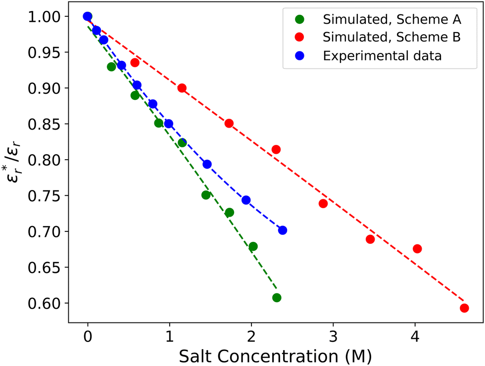Fig. 4 The ratio of the dielectric of a salt solution ε_r* to that calculated for pure water ε_r, shown as a function of NaCl salt content. We show simulated data for both scheme A (Mao et al.²) and scheme B (Anderson et al.³) SDS models. Experimental data taken from Buchner et al.⁷⁰

6 Micellar solutions

In this section, we compare the differences in surfactant aggregation behaviour when standard water and polarisable water models are applied. We also compare the effect that polarisable water has on the two different SDS models discussed thus far. In their original papers, both models showed a fairly strong relationship between aggregation number and concentration. Therefore, in each case, calculations are performed at four different concentrations: 2.5, 5, 7.5 and 10 wt% (corresponding to molar concentrations 87, 173, 260 and 346 mM). Each simulation is conducted in a cubic box with edge length L = 20r_C, with a total number of beads n = 24 000. Details on the number of water and surfactant beads this corresponds to can be found in the ESI.†

6.1 Aggregation number

For each simulation, we calculate a weighted aggregation number, defined as N_W = 〈N²〉/〈N〉 where . Here N is the number of monomers in a given molecule, and P_micelle is the probability of finding a monomer existing in a micelle of size N. The use of the weighted aggregation number, as opposed to simply the aggregation number, better represents polydisperse systems and is also more comparable with the experimental aggregation number. For this calculation, we output trajectory information every 10 000 time steps.

The instantaneous aggregation number as a function of time step is shown in Fig. 5. We note that the micelles produced by scheme B (Anderson et al.³) are generally larger and more stable than those produced by scheme A (Mao et al.²).

Fig. 5 Weighted aggregation number N_W as a function of simulated time steps for different concentrations. We simulate using a standard water model and the polarisable water model. We also test two different SDS parameterizations A (Mao et al.²) and B (Anderson et al.³) with water coarse-graining applicable to each model.

We equilibrate our micellar solutions until the final aggregation number no longer appears to be changing with further simulation time steps. Fig. 6 shows the calculated aggregation numbers, where the weighted aggregation number is calculated from the final 100 000 time steps. This figure shows that we do not see a significant difference between the polarisable and standard water models, at least with regard to the instantaneous aggregation number. The experimental value of the aggregation number varies between different experimental methods but is usually reported as between ≈75–110 in this concentration range.^26,27,29,31 As reported in the original DPD studies, the aggregation number is underpredicted in Fig. 6 compared with experimental data. However, we note an increase in the average aggregation number with increasing concentration, which is in line with experimental observations.²⁹

Fig. 6 Final weighted aggregation number using aggregation data from the final 1 × 10⁵ time steps.

6.2 Pre-assembled micelles

In Section 6.1 we initialised our simulations with random initial configurations, allowing the surfactant molecules to equilibrate into aggregates. Besides the issue of the dielectric constant, one additional frequently proposed reason that aggregation numbers are underpredicted is related to equilibration issues. Equilibration issues are expected to be more significant for ionic surfactants (than nonionic ones) on account of the strong electrostatic repulsion involved between the surfactant head groups.

Therefore, we also study micelles which are pre-formed at aggregation numbers close to the experimentally known values. This allows us to analyse if there is any difference in the behaviour of the polarisable and non-polarisable models at larger aggregation numbers. While other authors have taken the approach of placing micelles in a structured arrangement at the start of a simulation, we take a more practical approach. We initially simulate for a short period during which we apply no electrostatic interactions (effectively turning the counterions and head groups into water beads). We find that in all cases this leads to the relatively quick formation of a single micelle in the simulation box, owing to the lack of head-group repulsion limiting the micelle size. We take this as equivalent to a pre-assembled micelle. Then we simply turn on the electrostatic interactions and equilibrate.

We perform these calculations using SDS scheme B only, conducting simulations in a box with edge length L = 15r_C. Fig. 7 shows the final aggregation number after approximately 4.5 × 10⁶ time-steps, relative to the aggregation number the micelle is initialised at. We observe that the micelles in the simulations containing the polarisable water model appear to be significantly more stable than the micelles using standard water. In the case of using standard water, at preassembled aggregation numbers of >60, the micelle breaks down into two different aggregates, while in the polarisable case, the micelle remains a single whole micelle.

Fig. 7 Final aggregation number of micelles which are pre-assembled into a single micelle.

Above the upper limit of aggregation numbers shown in Fig. 7 (N > 90), we find that the micelle fragments when the electrostatic interactions are switched on in both water models. However, we also note that the fragmentation becomes somewhat more random for larger initial micelle sizes. For example, a micelle with an initial size N = 100 may fragment into two or three micelles in independent simulations. We find that this is usually related to how evenly the first ‘split’ of the initial micelle is. For example, if the micelle initially fragments into two micelles of approximately equal size (resulting in N_W ≈ 50), then it will not divide any further. However, if it initially fragments unevenly, (e.g. N = 20 and N = 80), then the larger micelle may divide again. This behaviour could make it difficult to ascertain an equilibrium aggregation number N_W using this approach, due to the randomness in how larger micelles can fragment.

6.2.1 Micelle shape. The shape of SDS micelles has been extensively studied experimentally using small-angle neutron^{21–26,29–31} and X-ray^32,33 scattering. It can generally be concluded⁷⁴ that experimental data shows that micelles are spherical or nearly spherical at most concentrations in the micellar range. However, at very high concentrations the average aggregation number can increase, and for SDS experimental results are interpreted to show a transition to ‘worm’-like or ‘rod’-like micelles, at aggregation numbers around N ≈ 130.²⁸ This transition takes place at larger concentrations and larger aggregation numbers than those used in this study. Therefore, we expect our simulated micelles to be relatively spherical.

We can quantitatively determine the degree of sphericalness of the micelles in these simulations by calculating the eccentricity e, which we define using the moment of inertia of the micelle:

where I_min is the smallest moment of inertia in any dimension and I_Avg is the average over all dimensions. A value of e = 0 corresponds to a perfectly spherical micelle. Fig. 8a shows the value for e as a function of the final size N. We take the value for eccentricity for the micelles in non-polarisable water when N > 60 during the period of the simulation after the charges have been turned on, but before the micelle has not broken down into two aggregates. We also show the standard deviation for the measured eccentricity, which is intended to show how much fluctuation there is in the micelle shape over the measurement period. We see that the shape (and shape fluctuation) of the micelles in standard water and polarisable water are relatively similar, despite the difference in their relative stability.

Fig. 8 The eccentricity of micelles (a) using the Anderson et al.³ parameterization as a function of their size N, where the error bar represents the standard deviation over the measurement period. Figure (b) shows two examples of the micelle shape when aggregation number N = 90. Images taken from the same simulation at two different time steps. Note the bead colour indicates the bead type, where: CH₃ bead (pink), CH₂ bead (blue) and head group (purple).

In both models, the eccentricity value is relatively small, particularly within the range . This is in good agreement with the experimental measurements discussed above, which indicated relatively spherical micelles. The micelles are most spherical around the size of N ≈ 40, before increasing in eccentricity for larger N. The error bars plotted for large N indicate significant amounts of fluctuation in micelle shape. Fig. 8b highlights the variation in shape for aggregates at sizes N = 90, showing that the micelle varies from nearly completely spherical to almost rod-like (note that more details about the fluctuation of eccentricity over the simulation time can be found in the ESI†). This significant fluctuation in micelle shape has also been observed for SDS in molecular dynamics⁴⁴ and experimental studies.⁷⁵ Palazzesi et al. use molecular dynamics to also calculate the eccentricity of an SDS micelle with an aggregation number of N = 60, finding an average value of e = 0.154, which we note is in excellent agreement with our average value using DPD.

6.3 Dielectric constant

6.3.1 Bulk water. We investigate whether our polarisable water model is behaving correctly by calculating the dielectric constant of the solvent as a function of surfactant concentration. Note that only water molecules are involved in this calculation. The effect of surfactant concentration on the bulk water is shown in Fig. 9, in which we observe a decrease in the solvent relative permittivity with increasing surfactant concentrations. This behaviour is in agreement with experimental observations.^76,77 We also observe that there is relatively little difference in behaviour between the two surfactant molecules in the level of decrement. This gives us confidence that the water model is behaving as expected in the presence of surfactant, allowing us to investigate the dielectric constant across the domain in more detail.

Fig. 9 Decrease in dielectric constant ε_r of the bulk water molecules with increasing surfactant concentration.

6.3.2 As a function of distance from a micelle. It has been suggested in theoretical works⁷⁸ that there is a reduction in relative permittivity near charged surfaces. In contrast, molecular dynamics simulations have indicated that the solvent polarisability oscillates near the surface,^73,79 although these two pictures have been shown to agree with each other if the oscillations are spatially averaged, leading to an overall decrease in the permittivity near the surface.⁷³ Therefore, one might expect to observe the same effect near the surface of ionic micelles.

This decrease in relative permittivity has been suggested to arise from a variety of possible origins, including the orientational ordering of water molecules close to the surface^78,80,81 and a decrease in the density of water molecules due to the presence of counterions.^78,82 We propose that a reduction in ε leads to a reduction in charge screening between the head groups of surfactant molecules. Therefore, a greater number of counterions condense at the micelle surface (in comparison to a case in which there is no reduction) to screen electrostatic interactions between the negatively charged head groups. It is of interest that previous works,⁴¹ in which various MD water models and force fields have been investigated for SDS micelles, appear to illustrate a link between counterion condensation and water model. We note that the authors appear to report a higher degree of condensation when models with lower dielectric constants are chosen.

It is nontrivial to calculate the dielectric constant as a function of position in our micellar systems, which would allow us to assess this theory. The dielectric constant is fundamentally a macroscopic property, and it is an open area of research concerning how the relative permittivity can be studied for inhomogeneous systems. While for a bulk material one can use Fröhlich-Kirkwood theory (eqn (15)), in inhomogeneous systems this equation becomes invalid. However, some studies have successfully calculated dielectric profiles for systems in which there is some spatial symmetry, for example in lipid bilayer systems⁸³ or in slab geometries,⁷³ where one has to assume dipole fluctuations in different perpendicular layers are not directly coupled.

In a similar manner, we estimate the variation in the relative permittivity as a function distance from the micelle's surface, by calculating the mean square dipole m_B of an inner spherical region of radius R (where R = 0 is the micelle's centre of mass). We estimate

where V_S is the volume of a sphere of radius R. This is an approximate approach,⁸⁴ which has also been used previously.^82,85 We perform a similar simulation to those described in Section 6.2, however, slightly increasing the box size from L = 15r_C to L = 20r_C to allow us to study the dielectric constant at a slightly longer range from the micelle. We simulate a micelle containing 60 surfactant molecules. When the electrostatic interactions are turned off, all surfactant molecules aggregate into a single micelle. Once the electrostatic interactions are turned on, the micelle loses a number of its monomers into the bulk, so that the aggregation number of the micelle we analyse is around N ≈ 56 over the analysis time.

Fig. 10 shows a plot of ε(R) as a function of R, where we also show the density profiles for the micelle and water. We see that the calculated value of ε(R) increases with distance from the micelle centre, and appears to be particularly tied with the increase in the water density. This suggests that indeed we do see a lower local dielectric constant closer to the micelle surface, which is strongly linked to an excluded volume effect due to the presence of ions.

Fig. 10 The density, plotted on the LHS axis, of various beads as a function of distance from a micelle of aggregation number N ≈ 56 using the Anderson model for the SDS surfactant. We also show (red) the dielectric constant of the water particles on the RHS axis.

6.4 Counter-ion behaviour

In this section, we investigate the impact of the water model and SDS model on the degree of disassociation of counterions. The degree of disassociation α potentially plays a role in the transition from spherical to rod-like micelles. The transition to elongated micelles can lead to viscoelastic behaviour, therefore accurate calculations for α are a crucial area of research. However, there exists a wide range of α values in the literature,^86–88 resulting from different experimental techniques and a lack of consensus over the definition of ‘dissociated ions’, an issue which has been discussed in literature.⁸⁷ However, values of around α = 0.3 are most commonly reported.^86,87 The calculation ofα from simulations is complicated by the fact that molecular dynamics simulations have shown that the value of α can depend on the choice of force field.⁴¹

Fig. 11 shows the radial distribution function (RDF) between the SO4 (SO⁴⁻) and NA (Na⁺) beads for different simulation cases. We observe that in the polarisable models, the head group and their counterion are closer than in the standard water case, and are significantly closer in the scheme B surfactant model. This shift in the radial distribution function (between the micelle and counter ions) has also been observed when comparing polarisable and non-polarisable MARTINI force fields.⁸⁹ While molecular dynamics simulations have reported⁴¹ that there are generally two distinct peaks within the first 0.6 nm, corresponding to the first two sodium shells, we only observe a single, broader peak. We attribute this to the coarse graining used in this work, which smears these into a single peak.

Fig. 11 Radial distribution function between the SO4 and NA beads for different simulation cases. All data presented for simulations at 10 wt%. Both SDS parameterisation schemes are shown: A (Mao et al.²) and B (Anderson et al.³).

We calculate the number of ions bound to the micelle β (where bound ions β = 1 − α), defining an ion to be bound if it is within a defined cut-off of one of the surfactant head groups. Molecular dynamics simulations⁴¹ report that, depending on the force field used, there exists on average around 60% (range 45–70% for the six force fields tested) of the sodium atoms within 0.6 nm of the RDF shell. We choose our cut-off distance to be R_Cut = 0.8R_C for the scheme A (Mao et al.²) SDS model, and R_Cut = 1R_C for scheme B (Anderson et al.³). Converted into real units, both of these cut-offs are approximately 0.57 nm, allowing for direct comparison with the molecular dynamics data.

Fig. 12 shows the fraction of ions bound to the micelles in each simulation case (note that we only consider ions associated with micelles in this calculation and surfactants which are considered free monomers are not included). The number of bound ions increases with concentration and is consistently higher in the polarisable models compared to standard water. The introduction of the polarisable model also causes the number of bound ions to be more comparable with both molecular dynamics data, and experimental data.

Fig. 12 Fraction of sodium ions within a defined cut-off range of head group beads. Cut-off distances of R_Cut = 1R_C in the Anderson et al.³ SDS model, and R_Cut = 0.8 R_C for the Mao et al.² model.

6.5 Micelle interactions

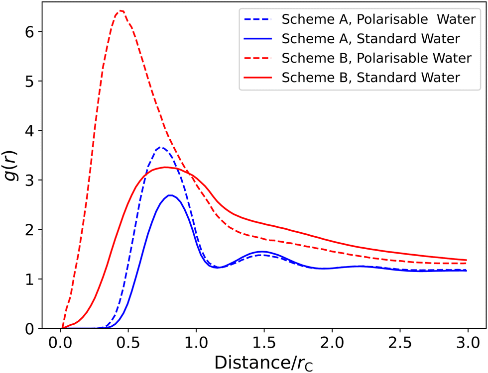
Finally, we briefly consider the impact of the polarisable water model on micelle–micelle interactions. The interactions between micelles are primarily influenced by the electrostatic interaction, as there is a net long-range force acting on micelles due to their net charge. We focus on scheme B for the surfactant and analyse the trajectories from simulations described earlier in this article (Section 6.1) for the micelles that form at 2.5 wt% SDS. At this concentration, we have three micelles, with an average aggregation number of N_W ≈ 25. The radial distribution function g(r) between the COM of micelles is calculated, and shown in Fig. 13 where we can see that there are only minor differences between the predictions from the two models. To further probe differences between the water models, we perform an additional set of simulations for a micellar system with added salt. The aim here was to bring the micelles slightly closer together, as in Fig. 13 it can be observed that they remain reasonably far apart during the whole measurement period.

Fig. 13 Radial distribution function g(r) between the COM of micelles in an aqueous solvent both with and without added NaCl salt.

We simulate a system consisting of two micelles of sizes N ≈ 64 and N ≈ 48, in a simulation box of size L = 23 which corresponds to a concentration of ≈2.5 wt% (85 mM). There is a small amount of fluctuation in the micelle sizes over the measurement period, but never more than ΔN ± 2. Here we can access larger micelle sizes, due to the enhanced head group screening that the salt provides. We then swap a number of the water particles for salt particles, which are defined in the same way as discussed in Section 5.2. We swap 200 water molecules for 100 sodium and 100 chloride ions, giving a salt concentration of ≈76 mM.

We generate the initial configuration of the two micelles by performing a similar trick to that discussed in Section 6.2, where we initially turn off the electrostatic charges to encourage micelle formation, and then turn them back on again once this has occurred to study their behaviour. In this case, rather than allowing a single micelle to form as before, we pause the simulation at the point where we have our two micelles, allowing us to use this as the starting configuration. Fig. 13 shows the radial distribution function g(r) between the COM of the two micelles. Here, with salt present, we see more variation between the two water models. It appears that, on average, the micelles get closer more often, an indication of the better electrostatic screening provided by the polarisable water model.

The potential of mean force (PMF), W(r), can be obtained from g(r)

W(r) = −k_BT ln g(r). (18)

From these simulations, W(r) is shown in Fig. 14 both with and without salt. Here, we have truncated the PMF when 1.5 < W(r), due to the high amount of uncertainty in our statistics at short micelle separation. The additional salt shields the micelles, such that (even though the micelles are larger) there is a lower W(r) for the systems with salt below a distance of 8 nm. We see very little difference in the PMF between the two water models for the solutions without added salt. However, in the salt solutions, we see that there is a reduction in the PMF in the range ≈6–8 nm. This is reflective of the differences we observe in the radial distribution function between the two water models.

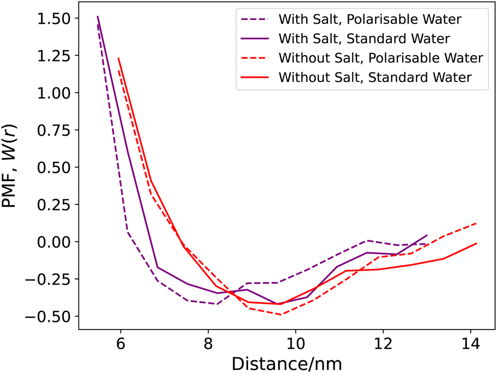Fig. 14 Potential of mean force between micelles, calculated using the RDF in Fig. 13.

Increases in the PMF at shorter distances are expected as the electrostatic repulsion grows as the charged micelles get closer. However, we note that there is a significant region in which W(r) < 0, implying that at larger distances there is an attractive force between the micelles. Interestingly, a description of intermicellar interactions in terms of a balance between a repulsive and an attractive potential has been proposed and discussed from both an experimental⁹⁰ and theoretical^91,92 point of view, but is not always observed in simulations.⁹³

7 Conclusions

We investigated the impact of polarisable water models on the aggregation behaviour of sodium dodecyl sulfate, allowing us to study whether the under-predicted aggregation numbers in DPD simulations can be improved with more complex water modelling. This polarisable water model was tested on simple salt solutions to confirm the correct dielectric behaviour of the model. Following this, the models were applied to the more complex surfactant solution cases.

We conclude that the underprediction of aggregate sizes in DPD models cannot alone be attributed to water modelling. However, there is evidence that polarisable water models produce micelles, which are more stable at larger aggregation numbers, and provide more accurate predictions for counterion behaviour. The use of polarisable water significantly increases the number of bound ions to the micelle, resulting in estimates for the number of bound ions much closer to experimental values, as well as being more in line with what is observed in molecular dynamics simulations. The observation that polarisable water leads to more stable micelles implies that equilibration is a key influence in the underprediction of aggregation numbers, particularly when our simulations are initialised with random positions for the surfactant molecules.

Furthermore, we show that the calculated dielectric constant increases as a function of distance from the surface of the micelle, as was initially postulated at the start of this article. This effect is likely due to the presence of counterions surrounding the micellar surface and is a phenomenon that would not normally be reflected in traditional DPD simulations using nonpolarisable water models.

It is possible that there are other simplifications in coarse-grained modelling that influence micelle formation and could be the source of aggregation under-prediction. For example, molecular dynamics⁹⁴ simulations of SDS micelles in water have shown that water molecules near the headgroup exhibit a distortion of the water–water hydrogen bonding. There have been some efforts to incorporate explicit hydrogen bonding into DPD, via the inclusion of a Morse potential,⁹⁵ and it would be interesting in future to assess whether models such as this have any impact on aggregation in DPD simulations.

We note that polarisable water models are more computationally demanding than the traditional DPD modelling approaches and therefore may not be appropriate for all systems of interest. However, for systems where counterion behaviour is a key aspect of interest, a polarisable water model is essential. We also note that our polarisable DPD model is still more computationally efficient than traditional fully atomistic approaches. We expect the models described here to find use in a range of diverse situations, including systems with charged surfaces, concentrated electrolyte solutions, and future studies of specific ion effects, as demonstrated, for example, in the Hofmeister series.

Author contributions

RH: conceptualization, data curation, formal analysis, investigation, methodology, software, validation, visualization, writing – original draft. CA: project administration, writing – review and editing. MW: funding acquisition, project administration, supervision, writing – review and editing.

Data availability

Data supporting this article have been uploaded as part of the ESI.†

Conflicts of interest

There are no conflicts to declare.

Acknowledgements

The authors would like to acknowledge the support of Durham University for the use of its HPC facility, Hamilton. RH would like to acknowledge support through an EPSRC/P&G funded Prosperity Partnership grant EP/V056891/1.

Notes and references

1. R. L. Hendrikse, C. Amador and M. R. Wilson, Soft Matter, 2024, 20, 6044–6058.
2. R. Mao, M.-T. Lee, A. Vishnyakov and A. V. Neimark, J. Phys. Chem. B, 2015, 119, 11673–11683.
3. R. L. Anderson, D. J. Bray, A. Del Regno, M. A. Seaton, A. S. Ferrante and P. B. Warren, J. Chem. Theory Comput., 2018, 14, 2633–2643.
4. D. Nivón-Ramírez, L. I. Reyes-García, R. Oviedo-Roa, R. Gómez-Balderas, C. Zuriaga-Monroy and J.-M. Martínez-Magadán, Colloids Surf., A, 2022, 645, 128867.
5. Z. Mai, E. Couallier, M. Rakib and B. Rousseau, J. Chem. Phys., 2014, 140, 204902.
6. R. L. Hendrikse, A. E. Bayly and P. K. Jimack, J. Phys. Chem. B, 2022, 126, 8058–8071.
7. S. J. Gray, M. Walker, R. Hendrikse and M. R. Wilson, Soft Matter, 2023, 19, 3092–3103.
8. V. Symeonidis, G. Em Karniadakis and B. Caswell, Phys. Rev. Lett., 2005, 95, 076001.
9. S. B. Chen, J. Phys. Chem. B, 2022, 126, 7184–7191.
10. H. Droghetti, I. Pagonabarraga, P. Carbone, P. Asinari and D. Marchisio, J. Chem. Phys., 2018, 149, 184903.
11. V. Symeonidis, G. E. Karniadakis and B. Caswell, J. Chem. Phys., 2006, 125, 184902.
12. R. Hendrikse, A. Bayly and P. Jimack, J. Chem. Phys., 2023, 158, 214906.
13. M. R. Wilson, G. Yu, T. D. Potter, M. Walker, S. J. Gray, J. Li and N. J. Boyd, Crystals, 2022, 12, 685.
14. T. L. Rodgers, O. Mihailova and F. R. Siperstein, J. Phys. Chem. B, 2011, 115, 10218–10227.
15. M. Lísal and J. K. Brennan, Langmuir, 2007, 23, 4809–4818.
16. M. Walker, A. J. Masters and M. R. Wilson, Phys. Chem. Chem. Phys., 2014, 16, 23074–23081.
17. M. Walker and M. R. Wilson, Soft Matter, 2016, 12, 8588–8594.
18. M. Walker and M. R. Wilson, Soft Matter, 2016, 12, 8876–8883.
19. M. Bates and M. Walker, Soft Matter, 2009, 5, 346–353.
20. M. A. Bates and M. Walker, Liq. Cryst., 2011, 38, 1749–1757.
21. B. Cabane, R. Duplessix and T. Zemb, J. Phys., 1985, 46, 2161–2178.
22. M. Bergstrom and J. S. Pedersen, Phys. Chem. Chem. Phys., 1999, 1, 4437–4446.
23. L. J. Magid, Z. Li and P. D. Butler, Langmuir, 2000, 16, 10028–10036.
24. M. Kakitani, T. Imae and M. Furusaka, J. Phys. Chem., 1995, 99, 16018–16023.
25. S. S. Berr and R. R. M. Jones, Langmuir, 1988, 4, 1247–1251.
26. M. Ludwig, R. Geisler, S. Prévost and R. von Klitzing, Molecules, 2021, 26, 4136.
27. R. Ranganathan, L. Tran and B. L. Bales, J. Phys. Chem. B, 2000, 104, 2260–2264.
28. B. L. Bales, L. Messina, A. Vidal, M. Peric and O. R. Nascimento, J. Phys. Chem. B, 1998, 102, 10347–10358.
29. B. Hammouda, J. Res. Natl. Inst. Stand. Technol., 2013, 118, 151–167.
30. S. Khodaparast, W. N. Sharratt, G. Tyagi, R. M. Dalgliesh, E. S. Robles and J. T. Cabral, J. Colloid Interface Sci., 2021, 582, 1116–1127.
31. V. Y. Bezzobotnov, S. Borbely, L. Cser, B. Farago, I. A. Gladkih, Y. M. Ostanevich and S. Vass, J. Phys. Chem., 1988, 92, 5738–5743.
32. S. L. Gawali, M. Zhang, S. Kumar, D. Ray, M. Basu, V. K. Aswal, D. Danino and P. A. Hassan, Langmuir, 2019, 35, 9867–9877.
33. Y. Mirgorod, A. Chekadanov and T. Dolenko, Chem. J. Mold., 2019, 14, 107–119.
34. P. Kékicheff, C. Grabielle-Madelmont and M. Ollivon, J. Colloid Interface Sci., 1989, 131, 112–132.
35. M. P. McDonald and W. E. Peel, J. Chem. Soc., Faraday Trans. 1, 1976, 72, 2274.
36. J. Bahadur, A. Das and D. Sen, J. Appl. Crystallogr., 2019, 52, 1169–1175.
37. J. Iyer and D. Blankschtein, J. Phys. Chem. B, 2014, 118, 2377–2388.
38. A. Goldsipe and D. Blankschtein, Langmuir, 2007, 23, 5953–5962.
39. S. Puvvada and D. Blankschtein, J. Phys. Chem., 1992, 96, 5567–5579.
40. E. A. Iakovleva, P. O. Sorina, E. A. Safonova and A. I. Victorov, Fluid Phase Equilib., 2022, 556, 113376.
41. X. Tang, P. H. Koenig and R. G. Larson, J. Phys. Chem. B, 2014, 118, 3864–3880.
42. B. J. Chun, J. I. Choi and S. S. Jang, Colloids Surf., A, 2015, 474, 36–43.
43. G. Roussel, C. Michaux and E. A. Perpète, J. Mol. Model., 2014, 20, 2469.
44. F. Palazzesi, M. Calvaresi and F. Zerbetto, Soft Matter, 2011, 7, 9148–9156.
45. D. L. Gurina and Y. A. Budkov, Colloids Surf., A, 2023, 676, 132200.
46. F. Leermakers and J. Lyklema, Colloids Surf., 1992, 67, 239–255.
47. V. G. de Bruijn, L. J. P. van den Broeke, F. A. M. Leermakers and J. T. F. Keurentjes, Langmuir, 2002, 18, 10467–10474.
48. Y. Lauw, F. A. M. Leermakers and M. A. Cohen Stuart, J. Phys. Chem. B, 2003, 107, 10912–10918.
49. S. Chanda and K. Ismail, Indian J. Chem., Sect. A: Inorg., Bio-inorg., Phys., Theor. Anal. Chem., 2009, 48, 775–780.
50. S. Pal, S. Balasubramanian and B. Bagchi, J. Chem. Phys., 2004, 120, 1912–1920.
51. H. Steinhoff, B. Kramm, G. Hess, C. Owerdieck and A. Redhardt, Biophys. J., 1993, 65, 1486–1495.
52. E. K. Peter and I. V. Pivkin, J. Chem. Phys., 2014, 141, 164506.
53. E. K. Peter, K. Lykov and I. V. Pivkin, Phys. Chem. Chem. Phys., 2015, 17, 24452–24461.
54. R. Vaiwala, S. Jadhav and R. Thaokar, Mol. Simul., 2018, 44, 540–550.
55. S. Chiacchiera, P. B. Warren, A. J. Masters and M. A. Seaton, Polarisable soft solvent models with applications in dissipative particle dynamics, 2024.
56. P. Español and P. Warren, Europhys. Lett., 1995, 30, 191–196.
57. A. P. Thompson, H. M. Aktulga, R. Berger, D. S. Bolintineanu, W. M. Brown, P. S. Crozier, P. J. In’t Veld, A. Kohlmeyer, S. G. Moore, T. D. Nguyen, R. Shan, M. J. Stevens, J. Tranchida, C. Trott and S. J. Plimpton, Comput. Phys. Commun., 2022, 271, 108171.
58. R. D. Groot, J. Chem. Phys., 2003, 118, 11265–11277.
59. P. B. Warren and A. Vlasov, J. Chem. Phys., 2014, 140, 084904.
60. M. González-Melchor, E. Mayoral, M. E. Velázquez and J. Alejandre, J. Chem. Phys., 2006, 125, 224107.
61. S. O. Yesylevskyy, L. V. Schäfer, D. Sengupta and S. J. Marrink, PLoS Comput. Biol., 2010, 6, e1000810.
62. J. Michalowsky, L. V. Schäfer, C. Holm and J. Smiatek, J. Chem. Phys., 2017, 146, 054501.
63. M. Vögele, C. Holm and J. Smiatek, J. Mol. Liq., 2015, 212, 103–110.
64. J. Song, M. Ma, Y. Dong, M. Wan, W. Fang and L. Gao, J. Chem. Theory Comput., 2023, 19, 1864–1874.
65. A. Catte, M. R. Wilson, M. Walker and V. S. Oganesyan, Soft Matter, 2018, 14, 2796–2807.
66. X. Periole and S.-J. Marrink, in The Martini Coarse-Grained Force Field, ed. L. Monticelli and E. Salonen, Humana Press, Totowa, NJ, 2013, pp. 533–565.
67. J. G. Kirkwood, J. Chem. Phys., 1939, 7, 911–919.
68. H. Fröhlich, Theory of dielectrics: dielectrics constant and dielectric loss., Clarendon Press, Oxford, 2nd edn, 1958.
69. A. D. Sen, V. G. Anicich and T. Arakelian, J. Phys. D: Appl. Phys., 1992, 25, 516.
70. R. Buchner, G. T. Hefter and P. M. May, J. Phys. Chem. A, 1999, 103, 1–9.
71. S. Seal, K. Doblhoff-Dier and J. Meyer, J. Phys. Chem. B, 2019, 123, 9912–9921.
72. C. J. Shock, M. J. Stevens, A. L. Frischknecht and I. Nakamura, J. Chem. Phys., 2023, 159, 134507.
73. P. Zarzycki, J. Colloid Interface Sci., 2023, 645, 752–764.
74. S. Vass, J. S. Pedersen, J. Pleštil, P. Laggner, E. Rétfalvi, I. Varga and T. Gilányi, Langmuir, 2008, 24, 408–417.
75. S. Choudhury, P. K. Mondal, V. K. Sharma, S. Mitra, V. G. Sakai, R. Mukhopadhyay and S. K. Pal, J. Phys. Chem. B, 2015, 119, 10849–10857.
76. D. K. George, A. Charkhesht, O. A. Hull, A. Mishra, D. G. S. Capelluto, K. R. Mitchell-Koch and N. Q. Vinh, J. Phys. Chem. B, 2016, 120, 10757–10767.
77. P. Fernandez, S. Schrödle, R. Buchner and W. Kunz, ChemPhysChem, 2003, 4, 1065–1072.
78. E. Gongadze and A. Iglic̆, Bioelectrochemistry, 2012, 87, 199–203.
79. D. J. Bonthuis, S. Gekle and R. R. Netz, Phys. Rev. Lett., 2011, 107, 166102.
80. H. Zhu, F. Yang, Y. Zhu, A. Li, W. He, J. Huang and G. Li, RSC Adv., 2020, 10, 8628–8635.
81. H. Itoh and H. Sakuma, J. Chem. Phys., 2015, 142, 184703.
82. T. Sato, T. Sasaki, J. Ohnuki, K. Umezawa and M. Takano, Phys. Rev. Lett., 2018, 121, 206002.
83. F. Zhou and K. Schulten, J. Phys. Chem., 1995, 99, 2194–2207.
84. V. Ballenegger and J.-P. Hansen, J. Chem. Phys., 2005, 122, 114711.
85. J. Powles, R. Fowler and W. Evans, Chem. Phys. Lett., 1984, 107, 280–283.
86. S. Ikeda, Colloid Polym. Sci., 1991, 269, 49–61.
87. B. L. Bales, J. Phys. Chem. B, 2001, 105, 6798–6804.
88. B. Naskar, A. Dey and S. P. Moulik, J. Surfactants Deterg., 2013, 16, 785–794.
89. A. V. Sangwai and R. Sureshkumar, Langmuir, 2011, 27, 6628–6638.
90. M. Corti and V. Degiorgio, J. Phys. Chem., 1981, 85, 711–717.
91. I. Sogami and N. Ise, J. Chem. Phys., 1984, 81, 6320–6332.
92. I. Sogami, Phys. Lett. A, 1983, 96, 199–203.
93. S. Kawada, K. Fujimoto, N. Yoshii and S. Okazaki, J. Chem. Phys., 2017, 147, 084903.
94. C. D. Bruce, S. Senapati, M. L. Berkowitz, L. Perera and M. D. E. Forbes, J. Phys. Chem. B, 2002, 106, 10902–10907.
95. G. Kacar and G. de With, J. Mol. Liq., 2020, 302, 112581.

---

Footnote

† Electronic supplementary information (ESI) available. See DOI: https://doi.org/10.1039/d4sm00873a

---