 Open Access Article
Development and comparison of regression models for the determination of quality parameters in margarine spread samples using NIR spectroscopy†
Anita
Rácz
 *a,
Marietta
Fodor
b and
Károly
Héberger
 a
a
aPlasma Chemistry Research Group, Research Centre for Natural Sciences, Hungarian Academy of Sciences, Magyar tudósok körútja 2, H-1117 Budapest XI., Hungary. E-mail: racz.anita@ttk.mta.hu
bSzent István University, Faculty of Food Science, Department of Applied Chemistry, Villányi út 29-43, H-1118 Budapest XI., Hungary
First published on 24th May 2018
Abstract
Fat and dry material contents (connected to moisture) are one of the most important parameters in the quality control of butter, margarine and margarine spreads (dairy spreads). More than a hundred margarine samples were used to model their fat and dry material content based on Fourier transform-near infrared (FT-NIR) spectroscopy in transmission and reflectance modes for the quality control of margarine. We also carried out a systematic comparison of various modeling techniques such as PLS regression, principal component regression (PCR) and support vector machines (SVM). Moreover, three types of cross-validation, three types of variable selection and the effect of different spectral types (transmission and reflectance) were also compared with factorial ANOVA tests. We examined the effect of the applied datasets (calibration, test samples, and both sets) based on the original predicted values. Sum of ranking differences (SRD), a novel comparison tool, was applied for the task. We showed that the SRD values can be used as a promising and useful performance parameter for the ranking and evaluation of numerous regression models. Four datasets with 42–42 transmission and 34–34 reflectance models were used for the evaluations. Finally, we have found the best models in each case based on their SRD values. The properly validated SVM models proved to be the best for all of the four used datasets. Although the method comparison is data set dependent, the suggested methodology is applicable generally and unambiguously. These final models can be used for fast and easy quality control of margarine samples instead of the time-consuming original analytical techniques.
1. Introduction
1.1 Margarine and margarine spreads
Margarine and margarine spreads were invented in the 19th century and in the beginning they were thought to be healthier than butter, and thus they were intended to be a replacement for butter. Margarine usually contains 20–80 w/w% fat; however “light” margarine, with lower than 40 w/w% fat content, is very popular nowadays. Although there is a debate between butter and margarine spread consumers, one can conclude that margarine is a cheaper replacement product for butter on the market.1Fat and dry material contents (connected to moisture) are one of the most important parameters of quality control of butter, margarine and margarine spreads (dairy spreads). The production process requires continuous control. The original analytical techniques for the determination of fat and dry material content are very time-consuming. The invention of these methods dates back to the nineties and the previous decade. Standard methods are unfortunately still based on these measurements. On the other hand, environmentally safer methods, which can decrease the amount of energy and the used solutions, are widely used nowadays instead of the original techniques. Fourier transform-near infrared (FT-NIR) measurements are one of these commonly used environmentally friendly and time-efficient substituents. FT-NIR is a non-destructive analysis for liquid, solid and colloidal (such as margarine) samples, and it can be applied as an on-line tool in the process control. In the past few decades several articles were published on this topic with the use of different spectroscopy related analytical methods for this area of food products. A short summary of these publications can be found in Table 1. It is interesting that the betterment of standard classical methods is based on exclusively spectroscopic methods. The majority of the related articles deals with classification and quantitative analysis (quality control) of these products.
| Author | Product | Determination | Methoda |
|---|---|---|---|
| a Abbreviations: ATR = attenuated total reflectance; HATR = horizontal-ATR; MIR = mid-infrared spectroscopy. | |||
| Evers et al.37 | Butter | Moisture, solid-not-fat (SNF) | Classical analysis (standard methods) |
| van de Voort et al.38 | Mayonnaise, peanut butter | Fat, moisture | FT-IR |
| van de Voort et al.39 | Butter | Fat, moisture | FT-IR (ATR) |
| Safar et al.40 | Margarine, butter, edible oil | Classification of products | FT-IR |
| Wilson41 | Margarine | trans-Fatty acid | HATR FT-IR |
| Hernández-Martínez et al.42 | Margarine | trans-Fatty acid | HATR FT-IR |
| Da Costa Filho43 | Edible oil | trans-Fatty acid | HATR FT-IR |
| Rohman and Man44 | Edible oil and fat | Counterfeit of products | FT-IR (MIR) |
| Vlachos et al.45 | Edible oil and fat | Counterfeit of products | FT-IR (MIR) |
| Hermida et al.46 | Butter | Fat, moisture, solid-not-fat (SNF) | FT-NIR |
| Yang, Irudayaraj and Paradkar47 | Edible oil | Classification of products | FT-IR, FT-NIR, Raman |
1.2 Chemometric analysis of NIR spectral data
Although with the use of IR or MIR spectroscopy, we have the opportunity to assign the peaks to compounds or properties, in the case of NIR spectroscopy it is not possible in the same way. Some general rules or pieces of advice in the selection of the measurement protocol (transmission vs. reflectance measurement) can be found; however in some special cases (as in this study) both ways have some advantages. In most cases further, detailed analysis of the spectra is needed with the help of chemometrics. Namely, we need multivariate regression methods, which can make a linear connection between the experimental (target) data (such as fat, moisture, etc.) and the spectra. The most common ones (among others) are partial least squares (PLS) and principal component regression (PCR).2 In the model building phase we can use several options to select the most important variables, such as interval selection or genetic algorithms.3 These methods can greatly improve the initial model. For the complete model building we also need a validation procedure, which helps to prevent the so-called overfitting problem in the model building. There is a long lasting debate amongst scientists in different research fields about the usefulness and importance of the internal and external validation steps in regression analysis.4–6 Martens and Dardenne have made a conclusion about the importance of full cross-validation, which gives more reliable results than any test set or independent external set. However, the use of a verification external test set can be good in long-term, but it also gives uncertain estimates about the predictive performance of the model.7 Although the latter publication is almost twenty years old, the debate is still open. The final question will always be: which is the most important performance parameter that we need to take into account? How (based on what) can we make a final decision about our models?In our study we wanted not only to develop predictive models for the fat and dry material content of margarine spreads, but also to compare and make a final decision about the models based on sum of ranking differences (SRD) and ANOVA. Our aim was also to examine the difference or similarity between (i) different cross-validation techniques, (ii) different regression methods, (iii) different variable selection techniques and (iv) different NIR spectral modes (transmission and reflectance). It was important and interesting to see and evaluate how the other parameters depend on different spectral modes and how the different spectral modes affect the final models. We also wanted to search for better options instead of using only one of the opportunities of internal and external validation techniques. In this way we will provide a new perspective for the scientific community dealing with multivariate regression models.
The above mentioned parameters are essential for regression model building, and thus one can use our conclusions and findings to save more time, money and energy in other NIR spectroscopy related studies.
2. Results and discussion
2.1 Regression model building and comparison of models
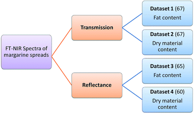
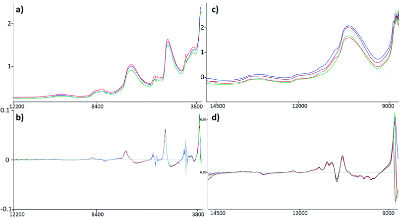
Four datasets were used for the regression model building, which can be seen in Fig. 1. Two types of spectra and two types of Y variables were used for the calibration models. The number of samples can be found in brackets.The regression models were optimized in the same way in each case. Derivation and mean centering were applied for the X variables and mean centering alone for the Y variables. A few examples of original and pre-processed spectra can be seen in Fig. 2.
In the case of transmission spectral datasets, 42–42 regression models (42 for the fat content and 42 for the dry material content, as well) were built and for reflectance spectral datasets 34–34 models were built. Different cross-validation techniques were used only in the case of transmission datasets; as a result the number of models (and combinations of parameters) is higher than in the case of reflectance spectra. The summary of the parameter combinations is provided in Table 2.
| Regression method | Validation | Variable selection |
|---|---|---|
| PLS | Random 5-fold CV (5-CV RANDOM) | iPLS/iPCR25 |
| PCR | Systematic 5-fold CV (5-CV SYST) | iPLS/iPCR50 |
| SVM | Leave-one-out CV (LOO) | Genetic algorithm (GA) |
| No selection (ALL) |
One example of the evaluated regression models can be seen in ESI, Fig. S1.†
2.2 Comparison of validation techniques
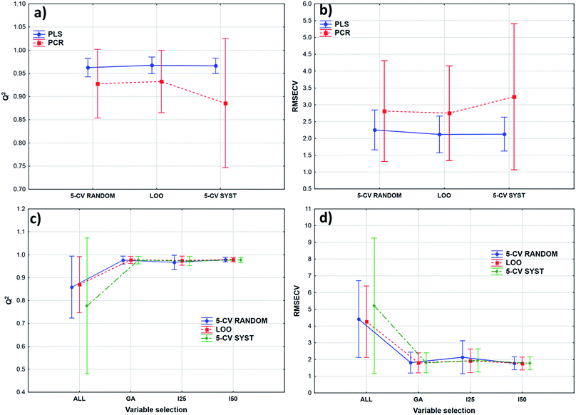
Transmission spectra were used to evaluate the effect of validation techniques on calibration model building process. The cross-validation methods are mentioned earlier in Table 2. Forty-two models were built in both cases with different parameters. Q2 (goodness of fit for the validated model) and RMSECV (root mean square error of cross-validation) values were used for the comparison of the models. The statistical analysis was carried out by ANOVA and factorial-ANOVA analysis of these performance parameters for the fat and dry material content models together. Factorial-ANOVA helped us to show the effect of validation methods with the different calibration methods and variable selections together. This way we can produce better visualized and more valuable plots. The effect of cross-validation techniques based on Q2 and RMSECV values was not statistically significant in both ways; p-values were 0.711 for Q2 and 0.901 for RMSECV (α = 0.05).In factorial-ANOVA at first we examined the effect of factors: three levels of cross-validation {leave-one-out (LOO) and fivefold cross-validation with systematic and random selection (5-CV random and 5-CV syst, respectively)} together with two levels of calibration methods (PCR and PLS regression). Then, we also compared the effect of cross-validation with four levels of variable selection techniques (VS): without VS (ALL), genetic algorithms (GA), and interval selection with splits 25 and 50 (I25 and I50, respectively). In both studies the effect of cross-validation methods remained insignificant (at the 5% level). Fig. 3 shows the results of factorial-ANOVA in the case of calibration methods (a and b) and variable selection techniques (c and d) together with cross-validations. It can clearly be seen in Fig. 3(a) and (b) that the PCR method is less certain because of the larger confidence intervals (95%). The PLS method was much more reliable in this sense for Q2 and RMSECV values as well. We can also see the difference between the confidence intervals (95%) of the models without any variable selection protocol or with variable selection. It means that the goodness of the models was increased with the variable selection techniques and the confidence intervals were decreased as well.
The smaller Q2 (and the larger RMSECV) necessitates some form of variable selection.
2.3 Comparison of models for the different datasets
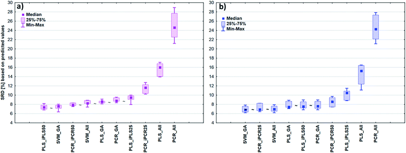
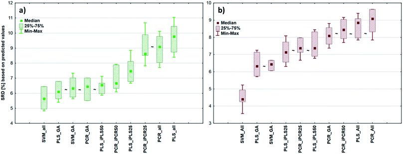
After the building of regression models with different parameters, we intended to find the best model(s) in each case and rank all the calibration models. The regression models were assigned to the datasets with the different spectral types and Y variables (fat and dry material content). The models were compared with SRD and the comparison was based on the cross-validated predicted values of the samples. The references or gold standard for SRD was the measured values (reference values). The predicted values of the external validation samples were also used in this section together with the internal sets, because in this way we can increase the robustness of the comparison. Nineteen and sixteen external test validation samples for the transmission datasets and sixteen and eight test validation samples for the reflectance datasets were used in the case of fat and dry material content models respectively. On the other hand, we aimed to show that SRD values can be used as performance parameters as well with the fusion of internal and external test results. In this case it can be more informative about the calibration models on its own. Further discussion about internal vs. external sets follows in the next section.In the case of transmission datasets, the results can be seen in Fig. 4(a) and (b). Box and whisker plots were used for the visualization of SRD values (the smaller the better). Sevenfold cross-validation was also applied in the SRD protocol; thus the SRD values can be plotted in this type of graph. Fig. 4 shows that the best models were the PLS regression one with iPLS50 variable selection and SVM regression with a genetic algorithm. The latter one was among the best ones not just in one but both cases, because there was no significant difference between SVM-GA and the next one, which was a PCR model (significance was tested by a Wilcoxon matched pair test, α = 0.05). PLS and PCR models without any variable selection method were the worst ones. However, if we do not use any variable selection technique in the case of SVM, we can still obtain a reliable regression model. SVM-All models were at the third and fourth places. The R2 and Q2 values of the best models were checked: 0.986 and 0.970 for the PLS-iPLS50 model respectively. In the same way they were 0.990 and 0.989 for the SVM-GA model, respectively. The fact that SRD did not choose wrong models, also verifies the SRD approach, if we compare it with the original or commonly used performance parameters. Finally, we can conclude that we can determine fat and dry material content based on these chosen models successfully. It is not feasible to use all wavelengths; it is better to use fewer intervals.
In the case of reflectance datasets, the protocol of comparison was the same as above. Here, eleven and eight external test validation samples were used in the case of fat and dry material content models, respectively. The final results for fat and dry material content can be seen in Fig. 5. Here SVM-All models without any variable selection method were clearly the best ones amongst the others. These models in (a) and (b) cases were significantly better than the other models. The SVM-All model for fat content determination has an R2 value of 0.991 and a Q2 value of 0.982. In the case of dry material content, the R2 and Q2 values of the SVM-All model were 0.992 and 0.979, respectively.
It can also be seen that the difference between the worst PLS and PCR models was smaller compared to the previous cases, but still, these models were not applicable for a successful calibration. On the other hand, SVM models were validated properly and these models can be applied in quality control procedures as well. SVM does not need/involve variable selection.
The average of the frequently used performance parameters of the models can be found in the ESI (Table S2).†
2.4 SRD and factorial ANOVA analysis of the four model sets together
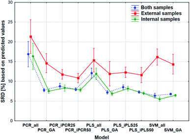
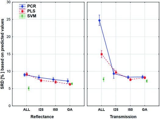
The comparison was also made by all of the four model sets (based on Fig. 1) together, which means that we used the predicted values of the samples from the 152 models (42–42 models for transmission spectral datasets and 34–34 models for reflectance spectral dataset). In the four SRD evaluations the reference column always contained the measured reference values. The internal and external samples were used together and separately as well, because in this way we could evaluate the effect of the internal and external sets on the final decision about the models. Factorial-ANOVA was applied for the examination of the SRD values. The different sample sets (both samples, external samples, and internal samples) and the different models were used as indicators. The effects of these two parameters were evaluated together and the result can be seen in Fig. 6. This plot shows that all SRD values of the external set are higher (worse) than those of the other two sample sets and it also has bigger confidence intervals for every model than the other sets. Although the shape of the line is quite the same for all of the three sample sets, if we make a decision about the models based on only the external set, we clearly omit one side of the information and it can mislead us, because of its uncertainty. A statistically significant difference was detected between the sample sets (both samples, external samples, internal samples).Factorial-ANOVA was used with other indicators as well. The effect of the regression methods, different variable selections and spectral types were examined in the following procedure. For this analysis both sample sets and the external set alone were used with their predicted values. For both sample sets, the results can be seen in Fig. 7.
The plot has two splits: one for the transmission and one for the reflectance spectral type. It can be clearly seen that the use of variable selection can cause more difference in SRD values, especially in the case of transmission spectra. The effect of the different regression methods is also larger, if we used the transmission spectra, but SVM was clearly better than the other methods in both cases. ANOVA also proved that in the case of SVM alone, variable selection has no significant effect. On the other hand, a largest improvement can be achieved in the case of PCR models with the variable selections if transmission spectra are used. The confidence intervals (95%) are smaller in the case of reflectance spectra, but they were not significant in the other type as well. However, the effects of different regression methods, variable selections and spectrum types were significant.
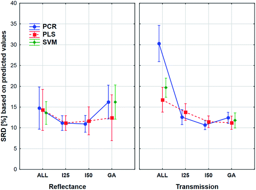
The aforementioned effects were examined in the same way with the use of the external sample set alone. We wanted to see, what is the difference between the application of the two sets. The results can be seen in Fig. 8.
Here the shapes of the lines (reflectance – “U” shape and transmittance – distorted “U” shape) are somewhat similar, although the confidence intervals (95%) are much larger in all cases compared to the previous one. It is also interesting to see that the tendency is not the same in the case of the genetic algorithm: the SRD values increase a little for the reflectance spectra, but this increase is larger in the case of transmission spectra. However, ANOVA can detect significant differences between the models, variable selections and spectrum types, and it can be clearly seen that the decision about the best ones is not at all obvious. Thus, it also verifies the conclusion that we cannot make a decision based on only the external test samples and their results. This conclusion corresponds to our earlier findings on two different case studies.5
The role of internal and external validation in the validation of models and calculation of predictive performance is still a debated issue in the fields of machine learning, chemometrics and any kind of modeling discipline. In the literature one can find several studies, which prefer the internal validation over the external one.8–10 However, other papers emphasize the importance of external sets.11,12
The debate continues: external validation based on a single split of the data set might not be so good as previously thought: metrics calculated from the test set could lead to random decisions.5 External validation is considered as the gold standard for checking the predictive ability of QSAR models, and others still think cross-validation is better suited for checking the predictive ability of QSAR models in order to avoid the loss of information from splitting of the data set into training and test sets.13
We used internal validation (cross-validation) and external sample sets (new, commercial samples) for the validation of our models. Our opinion based on the results of this work and previous findings is that making a final conclusion based only on the external test set can be misleading. We can assume that these new samples have a fifty–fifty chance of being a part of the same distribution as the calibration model or a part of another distribution. Therefore, we can obtain very good external results and very bad ones with equal probability. If the external set belongs to the same distribution as the earlier samples, external validation cannot add any new information as compared to inner validation. If the external set has been drawn from a different distribution one cannot use the earlier developed model(s) for prediction (without updating). The external test set cannot provide such a robust and reliable result alone as the internal validation. Reversely, if a model has bad quality parameters in the internal validation section, usually it will not be able to predict external samples, either. In some seldom cases an external set may provide somewhat better performance.
In our opinion SVM is a very promising tool for multivariate modeling and we can easily exclude the opportunity of overfitting with a proper validation protocol. On the other hand, SVM needs more regularization parameters than PLS, but this can be handled with proper validation. However, we also found some cases, where SVM is worse than the other techniques. One can also find publications, which are denying the overfitting “feature” of the method (see e.g.Table 2 in ref. 14).
Our conclusion does not contradict the literature suggestions. We would not neglect the usage of an external set, but we have to be careful with it. A decision based solely on an external set is equivalent to delivering our models to a random choice. Our conclusion provides a new perspective to the debating situation in this issue.
3. Experimental
3.1 Samples
Four datasets were used for the regression analysis based on the dependent (Y) variable (fat content or dry material content) and measurement type (transmission and reflectance). The final number of the samples was always based on the experimental measurements, and thus in the case of reflectance spectra the final numbers were 65 (fat content) and 60 (dry material content). In the case of transmission spectra, we used 67 samples for both of the fat and dry material content. The number of samples was different according to the mode of NIR measurements. The measurements were done in a continuous way and some of the samples were deteriorated during the course of measurements. This cannot cause any problem in the following steps, because the models should work on every type of sample and batch. The datasets contained original (commercially available) and mixed samples as well, because we wanted to cover the total concentration range properly with a sufficient number of samples. Mixed samples were made from the original ones with a well-determined mass-ratio (1![[thin space (1/6-em)]](https://www.rsc.org/images/entities/char_2009.gif) :
:![[thin space (1/6-em)]](https://www.rsc.org/images/entities/char_2009.gif) 1, 6
1, 6![[thin space (1/6-em)]](https://www.rsc.org/images/entities/char_2009.gif) :
:![[thin space (1/6-em)]](https://www.rsc.org/images/entities/char_2009.gif) 4, 7
4, 7![[thin space (1/6-em)]](https://www.rsc.org/images/entities/char_2009.gif) :
:![[thin space (1/6-em)]](https://www.rsc.org/images/entities/char_2009.gif) 3, and 8
3, and 8![[thin space (1/6-em)]](https://www.rsc.org/images/entities/char_2009.gif) :
:![[thin space (1/6-em)]](https://www.rsc.org/images/entities/char_2009.gif) 2) for the mixing. The amount of original samples was measured with analytical precision for the mixtures; then, the mixtures were homogenized carefully. The ranges of the fat and dry material content can be seen in ESI Table S1.† Using mixed samples is a common thing especially in the field of NIR measurements, because there are several cases when the number of original samples is limited and it will not be enough for a robust model. The situation is always case dependent, but the mixed samples can help us to solve this type of problem in an easy way. The mixed samples are always in the same distribution.
2) for the mixing. The amount of original samples was measured with analytical precision for the mixtures; then, the mixtures were homogenized carefully. The ranges of the fat and dry material content can be seen in ESI Table S1.† Using mixed samples is a common thing especially in the field of NIR measurements, because there are several cases when the number of original samples is limited and it will not be enough for a robust model. The situation is always case dependent, but the mixed samples can help us to solve this type of problem in an easy way. The mixed samples are always in the same distribution.
3.2 Experimental data
The determination of dry material content of the margarine spreads is based on the ISO 3727-1:2002 international standard. The measurements were carried out in Petri dishes. The homogenized samples with an exact amount of ignited silica sand were put into the dishes. The samples were heated at 102 °C for one hour. After careful cooling in a glass-desiccator the samples were placed back in the drying oven for 30 min per round till any mass differences were detected. For the fat content another standard method, ISO 17189:2004, was used, which is based on cold extraction. The main step of the analysis was the following: the samples were homogenized and put into Erlenmeyer-flasks. The extraction process was done with petroleum ether and with the help of ethanol the phases were separated. The extraction was carried out in four steps. Then a water bath for the evaporation, drying oven and desiccator were used to reach the final form and final mass of the samples.The measured concentrations are given in w/w%. Measurement duplicates were used for each sample. If the value was significantly different from the nominal concentration, more additional duplicates were used for the analysis. The relative standard deviation was 1.59 w/w% and 1.30 w/w% for fat and dry material content respectively. The original samples were not always the same in the case of reflectance and transmission spectra, because there was a time shift between the two types of measurements, and some of the original samples were expired and thus we couldn't use them again. This cannot cause any problem in the measurement of authenticity, because the models should work on all the different samples that are commercially available.
The applied compounds for the experiments were ignited silica sand (puriss, Spektrum 3D, Hungary), ethanol (100 v/v%, Reanal, Hungary) and petroleum ether (40–65 °C, Reanal, Hungary).
3.3 FT-NIR measurements
A Bruker MPA™ Multipurpose Fourier-transform near-infrared spectroscopy (FT-NIR) analyzer (Bruker Optik GmbH, Ettlingen, Germany) was used for FT-NIR measurements. The device is equipped with a quartz beam splitter and an integrated Rocksolid™ interferometer. The spectral resolution was 8 cm−1 and the scanner speed was 10 kHz.In transmission mode (800–1100 nm or 12![[thin space (1/6-em)]](https://www.rsc.org/images/entities/char_2009.gif) 500–9000 cm−1) an outer transmission interface and Si-diode detector were used and the homogenized samples were placed in Petri dishes, as sample compartments. In this case the device scanned the sample 64 times and an average spectrum was constructed from the scans.
500–9000 cm−1) an outer transmission interface and Si-diode detector were used and the homogenized samples were placed in Petri dishes, as sample compartments. In this case the device scanned the sample 64 times and an average spectrum was constructed from the scans.
In diffuse reflectance mode a rotatable sample wheel and a PbS detector were used. In this case a part of the infrared light is absorbed on the layer of the sample, while the other part is reflected and it goes to the detector. In this case each spectrum was the average spectrum of 32 subsequent scans.
The comparison of the two different spectral types can be seen in the Results and discussion part as well (Fig. 2). Reflectance spectra are richer in peaks, but transmission spectra are used more often for this type of sample.
Every sample had two duplicates. The average of the duplicates' spectra was used for the multivariate calibration.
3.4 Multivariate regression methods
Multivariate regression analysis of spectral datasets is the essential part of this examination, because the information in NIR spectral data can be extracted only this way. The most commonly used techniques are partial least squares regression and principal component regression; however nowadays some other techniques such as the so-called machine learning methods (for example support vector machines) or tree-type (decision tree) algorithms are also getting more and more popular.15–17 In our study principal component regression, partial least-squares regression and support vector machine regression were used, and thus in the following part we summarize these techniques briefly.Principal component regression (PCR) is very close to multilinear regression (MLR) and principal component analysis (PCA). The basic idea of PCR is divided into two steps: (a) to calculate the principal components from the original variables and (b) use the new virtual variables (PC scores) for the regression model building with the typical and well-known MLR equation:
| Y = Xb + E | (1) |
The advantage of this method is that it suppresses the spectral collinearity. However, there is no guarantee that the calculated PCs are correlated with the reference variable Y.18,19
Partial least-squares regression (PLS-R) is the most frequently used multivariate regression technique since the past few decades in the field of NIR spectroscopy. A tutorial paper of Geladi and Kowalski gives a very good explanation of this method.2 The increasing popularity of PLS dates back to that publication, since PLS regression can be considered as the basic tool for multivariate regression. The basic idea of PLS-R is a matrix transformation, which divides the original X and Y matrices into the multiplication of score and loading matrices in quite the same way as PCA works. They are called the outer relations.2,20 PLS regression can use the new “latent” variables (T and U) for the prediction of Y values.21 There is an inner relationship as well between the PLS components (U and T) of the X and Y matrices, which can be described with an equation similar to eqn (1). The determination of the number of components is an essential part of model building. We can easily overfit or underfit the models, if we do not pay attention to the harmony/parsimony tradeoff.22 A commonly used method for this purpose is the global or local minimum value of the root mean square error of cross-validation (RMSECV) or predictive error of sum of squares (PRESS).
We can find more opportunities in the extended literature of this field, for example the randomization test, the decision based on eigenvalues, etc.23,24 In this study, the first local minimum of RMSECV values was used, and in the lack of a minimum value, the starting point of a plateau was used based on visual inspection.
Support vector machine (SVM) regression was also used for the model building. This method belongs to machine learning techniques, and it is a younger one and not yet as popular as PLS or PCR. However, they can have high potential, because in the past few decades the developments and applications of machine learning (especially SVM) algorithms are rapidly increasing.25,26 This is the reason why we also wanted to test and compare this method with the others. SVM finds a relationship between the regressors and the Y values (dependent ones). SVM projects the original data into a space of higher (rather than lower) dimensions (feature space) using a suitable kernel function18,27 (the most popular functions include polynomial kernels and the Gaussian radial basis function). We have to note that SVM models can be very sensitive to overfitting, and several meta parameter combinations provide the same results; thus, a careful validation is advised.
3.5 Variable selection methods
Variable selection is an important part of the regression model building in the case of FT-NIR spectroscopy, because we have to select those important segments of the spectrum, which are connected to the real information and not just noise. Thus, the main reason for using these methods is to reduce the dimension of the original variable set and on the other hand we can increase the goodness of our model. Most of these methods use different parameters for this purpose such as R2, Mallows Cp, etc. In the case of PLS regression we can also use regression coefficients (b) and PLS loading vectors.Some complex methods for selection can be the genetic algorithm (GA) or interval PLS/PCR as well. Usually the spectra can be divided into several equal parts (e.g. 10, 20, and 40). Working with intervals or windows can be a better choice because the spectral wavelengths are not independent of each other.28,29 Interval selection is highly recommended especially in the case of GA.3 The final decision about the best parts can be made by RMSECV, R2 or its cross-validated counterpart (Q2). In our study GA, iPLS and iPCR with 10 and 25 intervals were used in the model building phase.
3.6 Validation techniques
Cross-validation is probably the most commonly used method for the estimation of prediction error. The typical realizations of cross-validation are the following: (a) random subsets, (b) systematic (Venetian blind), (c) contiguous blocks, and (d) leave-one-out. However, several other forms can be found in the work of Bro et al.23 In the case of n-fold (leave-many-out) cross-validation, the most recommended versions are five- and ten-fold splits.30 Other resampling methods can also be found in the literature for validation protocols such as Y- and X-scrambling of the dataset,31 bootstrap32 or repeated double cross-validation.33 In this study fivefold cross-validation with randomized and systematic forms and leave-one-out cross-validation were used for the validation of the models and compared with other statistical methods. Random subsets and systematic and contiguous blocks can be seen in Fig. 9 in detail.In the case of leave-one-out, all samples are excluded once and only once, whereas the others are used for calibration (see Fig. 9). It means that if the number of samples is N, we have to repeat the cross-validation N times.
In this study, Unscrambler X 10.3 (Camo Software, Oslo, Norway) was used for the regression model building and the validation of models.
3.7 Sum of ranking differences
Sum of ranking differences (SRD) is a novel algorithm to compare methods, models, and any type of sample and variable fairly.34,35 The method is entirely general. The basic idea is the following: in the input matrix the samples are placed in the rows and the variables (methods and models) are in the columns. We always compare the columns of a matrix (i.e. the variables). At first, a reference (gold standard) column should be added to the end of the matrix, which can contain exact reference values or average, minimum/maximum values of the rows (samples). Then the samples in every column are ranked by increasing magnitude. The differences between the ranks of a variable (model) and the rank of the reference are calculated in each case (for each variable). The absolute values of differences are summed together for each column. This will be the SRD value of the column (model) which can be compared to the others. The smaller is the SRD value, the better is the column (model). The method is explained in detail with an animation in the work of Bajusz et al.36 SRD was used with a home-made Microsoft EXCEL VBA macro, which is freely available on the Internet as well: http://aki.ttk.mta.hu/srd.3.8 Model building workflow
Outlier samples were selected based on principal component analysis (with the 95% confidence limit). Finally, only a few samples (2–3) were omitted because of this reason. In the model building phase the selection of the number of components (in PLS and PCR) was based on the aforementioned protocol in this section. PLS Toolbox 7.9 (Eigenvector Research, Inc., Wenatchee, WA, USA) was used for interval PLS, interval PCR and a genetic algorithm. In the case of interval PLS and PCR the data splits contained 25 or 50 variables in two separate versions. For the genetic algorithm the width of the window was 50 variables. In the GA procedure all the other parameters were applied based on our previous study.20 For SVM models a grid search workflow was used to find the best values of regularization parameters, e.g. C and gamma. This protocol is implemented in Unscrambler X to find the combination of parameters, where the RMSECV value of the models is the lowest. This algorithm was used for all of the SVM models.4. Conclusion
Based on the FT-NIR spectra of margarine spread samples, their fat and dry material content can be determined successfully and precisely. The properly validated final models for the fat and dry material content of margarine spread samples are suitable for the quality control of these products. The validated SVM models were among the best ones in each case. All of the best models had determination coefficients (R2) and their cross-validated (Q2) values above 0.97.There is no statistically significant difference between leave-one-out, randomized and systematic fivefold cross-validations. It means that based on our findings we can choose whatever the cross-validation type we want, and the results will not be significantly different. Furthermore, external sample sets alone can give uncertain and biased results with higher error values. However, external sets have different behavior; thus, the models should be applicable to them as well. To solve this problem, the final decision about the models based on FT-NIR spectra should be made by using external and internal samples and their predicted values together. For this purpose, the SRD values can be successfully used and can be considered as a novel performance parameter as well. They can give consistent, properly validated and reliable results about the models.
The effects of the applied regression models, variable selection techniques and spectral types were significant in each case. We can conclude that the variable selection techniques were useful in the case of transmission spectra and also in the case of the PCR method. Moreover, the effect of variable selection for SVM alone was not significant.
The applied statistical analysis protocol is applicable for other (even special or complicated) datasets as well. The SRD methodology is entirely general and it can be used not just as a performance parameter but in other comparison studies as well.
Conflicts of interest
There are no conflicts to declare.Acknowledgements
The authors thank the support of the National Research, Development and Innovation Office of Hungary (OTKA, contracts No. K 119269 and KH 125608). We also acknowledge the technical support of Adrienn Somogyi and Csilla Biróova.References
- J. W. Fuguay, P. F. Fox and P. L. H. McSweeney, Encyclopedia of Diary Sciences, Elsevier, 2011 Search PubMed.
- P. Geladi and B. R. Kowalski, Anal. Chim. Acta, 1986, 185, 1–17 CrossRef.
- C. M. Andersen and R. Bro, J. Chemom., 2010, 24, 728–737 CrossRef.
- P. Gramatica, QSAR Comb. Sci., 2007, 26, 694–701 CrossRef.
- A. Rácz, D. Bajusz and K. Héberger, SAR QSAR Environ. Res., 2015, 26, 683–700 CrossRef PubMed.
- D. Baumann and K. Baumann, J. Cheminf., 2014, 6, 47 Search PubMed.
- H. A. Martens and P. Dardenne, Chemom. Intell. Lab. Syst., 1998, 44, 99–121 CrossRef.
- M. Gütlein, C. Helma, A. Karwath and S. Kramer, Mol. Inf., 2013, 32, 516–528 CrossRef PubMed.
- T. Hastie, R. Tibshirani and J. Friedman, in The Elements of Statistical Learning: Data Mining, Inference, and Prediction, Springer New York LLC, 2nd edn, 2009, pp. 241–249 Search PubMed.
- R. Kohavi, in IJCAI'95 Proceedings of the 14th International Joint Conference on Artificial Intelligence, 1995, pp. 1137–1143 Search PubMed.
- P. Gramatica, Mol. Inf., 2014, 33, 311–314 CrossRef PubMed.
- K. H. Esbensen and P. Geladi, J. Chemom., 2010, 24, 168–187 CrossRef.
- K. Roy, P. Ambure, S. Kar and P. K. Ojha, J. Chemom., 2018, 32, e2992 CrossRef.
- P. S. Gromski, H. Muhamadali, D. I. Ellis, Y. Xu, E. Correa, M. L. Turner and R. Goodacre, Anal. Chim. Acta, 2015, 879, 10–23 CrossRef PubMed.
- U. Thissen, M. Pepers, B. Üstün, W. J. Melssen and L. M. C. Buydens, Chemom. Intell. Lab. Syst., 2004, 73, 169–179 CrossRef.
- X. Niu, Z. Zhao, K. Jia and X. Li, Food Chem., 2012, 133, 592–597 CrossRef PubMed.
- E. Teye, X. Huang, H. Dai and Q. Chen, Spectrochim. Acta, Part A, 2013, 114, 183–189 CrossRef PubMed.
- Y. Roggo, P. Chalus, L. Maurer, C. Lema-Martinez, A. Edmond and N. Jent, J. Pharm. Biomed. Anal., 2007, 44, 683–700 CrossRef PubMed.
- T. Naes, T. Isaksson, T. Fearn and T. Davies, A User Friendly Guide to Multivariate Calibration and Classification, NIR Publications, Chichester, UK, 2002 Search PubMed.
- A. Rácz, A. Vass, K. Héberger and M. Fodor, Anal. Bioanal. Chem., 2015, 407, 2887–2898 CrossRef PubMed.
- R. G. Brereton and G. R. Lloyd, J. Chemom., 2014, 28, 213–225 CrossRef.
- F. Stout, M. R. Baines and J. H. Kalivas, J. Chemom., 2006, 20, 464–475 CrossRef.
- R. Bro, K. Kjeldahl, A. K. Smilde and H. A. L. Kiers, Anal. Bioanal. Chem., 2008, 390, 1241–1251 CrossRef PubMed.
- S. Wiklund, D. Nilsson, L. Eriksson, M. Sjöström, S. Wold and K. Faber, J. Chemom., 2007, 21, 427–439 CrossRef.
- A. J. Smola and B. Schölkopf, Stat. Comput., 2004, 14, 199–222 CrossRef.
- G.-B. Huang, H. Zhou, X. Ding and R. Zhang, IEEE Trans. Syst. Man Cybern. B Cybern., 2012, 42, 513–529 Search PubMed.
- R. G. Brereton and G. R. Lloyd, Analyst, 2009, 135, 230–267 RSC.
- C. V. Di Anibal, M. P. Callao and I. Ruisánchez, Talanta, 2011, 86, 316–323 CrossRef PubMed.
- L. Nørgaard, A. Saudland, J. Wagner, J. P. Nielsen, L. Munck and S. B. Engelsen, Appl. Spectrosc., 2000, 54, 413–419 CrossRef.
- T. Hastie, R. Tibshirani and J. Friedman, in The Elements of Statistical Learning; Data Mining, Inference, and Prediction, Springer, New York, 2001, pp. 214–216 Search PubMed.
- C. Rücker, G. Rücker and M. Meringer, J. Chem. Inf. Model., 2007, 47, 2345–2357 CrossRef PubMed.
- R. Wehrens, H. Putter and L. M. C. Buydens, Chemom. Intell. Lab. Syst., 2000, 54, 35–52 CrossRef.
- P. Filzmoser, B. Liebmann and K. Varmuza, J. Chemom., 2009, 23, 160–171 CrossRef.
- K. Héberger, Trac. Trends Anal. Chem., 2010, 29, 101–109 CrossRef.
- K. Kollár-Hunek and K. Héberger, Chemom. Intell. Lab. Syst., 2013, 127, 139–146 CrossRef.
- D. Bajusz, A. Rácz and K. Héberger, J. Cheminf., 2015, 7, 20 Search PubMed.
- J. M. Evers, R. A. Crawford, L. M. Wightman and R. C. Kissling, Int. Dairy J., 2001, 11, 127–136 CrossRef.
- F. R. van de Voort, J. Sedman and A. A. Ismail, Food Chem., 1993, 48, 213–221 CrossRef.
- F. R. van de Voort, J. Sedman, G. Emo and A. A. Ismail, Food Res. Int., 1992, 25, 193–198 CrossRef.
- M. Safar, D. Bertrand, P. Robert, M. F. Devaux and C. Genot, J. Am. Oil Chem. Soc., 1994, 71, 371–377 CrossRef.
- R. H. Wilson, Trends Anal. Chem., 1990, 9, 127–131 CrossRef.
- M. Hernández-Martínez, T. Gallardo-Velázquez and G. Osorio-Revilla, Eur. Food Res. Technol., 2010, 231, 321–329 CrossRef.
- P. A. Da Costa Filho, Food Chem., 2014, 158, 1–7 CrossRef PubMed.
- A. Rohman and Y. B. C. Man, Food Res. Int., 2010, 43, 886–892 CrossRef.
- N. Vlachos, Y. Skopelitis, M. Psaroudaki, V. Konstantinidou, A. Chatzilazarou and E. Tegou, Anal. Chim. Acta, 2006, 573–574, 459–465 CrossRef PubMed.
- M. Hermida, J. M. Gonzalez, M. Sanchez and J. L. Rodriguez-Otero, Int. Dairy J., 2001, 11, 93–98 CrossRef.
- H. Yang, J. Irudayaraj and M. M. Paradkar, Food Chem., 2005, 93, 25–32 CrossRef.
Footnote |
| † Electronic supplementary information (ESI) available. See DOI: 10.1039/c8ay01055b |
| This journal is © The Royal Society of Chemistry 2018 |

