
 Open Access Article
 This Open Access Article is licensed under a
 Creative Commons Attribution 3.0 Unported Licence
Multi-stage freezing of HEUR polymer networks with magnetite nanoparticles†
A.
Campanella
*a,
O.
Holderer
a,
K. N.
Raftopoulos
b,
C. M.
Papadakis
b,
M. P.
Staropoli
c,
M. S.
Appavou
a,
P.
Müller-Buschbaum
b and
H.
Frielinghaus
a
aJCNS@FRMII, Lichtenbergstraße 1, 85747 Garching, Germany. E-mail: a.campanella@fz-juelich.de; Fax: +49 (0)8928910799
bTechnische Universität München, Physik-Department, Lehrstuhl für Funktionelle Materialien/Fachgebiet Physik weicher Materie, James-Franck-Straße 1, 85748 Garching, Germany
cJCNS-1, Forschungszentrum Jülich GmbH, 52425 Jülich, Germany
First published on 16th February 2016
Abstract
We observe a change in the segmental dynamics of hydrogels based on hydrophobically modified ethoxylated urethanes (HEUR) when hydrophobic magnetite nanoparticles (MNPs) are embedded in the hydrogels. The dynamics of the nanocomposite hydrogels is investigated using dielectric relaxation spectroscopy (DRS) and neutron spin echo (NSE) spectroscopy. The magnetic nanoparticles within the hydrophobic domains of the HEUR polymer network increase the size of these domains and their distance. The size increase leads to a dilution of the polymers close to the hydrophobic domain, allowing higher mobility of the smallest polymer blobs close to the “center”. This is reflected in the decrease of the activation energy of the β-process detected in the DRS data. The increase in distance leads to an increase of the size of the largest hydrophilic polymer blobs. Therefore, the segmental dynamics of the largest blobs is slowed down. At short time scales, i.e. 10−9 s < τ < 10−3 s, the suppression of the segmental dynamics is reflected in the α-relaxation processes detected in the DRS data and in the decrease of the relaxation rate Γ of the segmental motion in the NSE data with increasing concentration of magnetic nanoparticles. The stepwise (multi-stage) freezing of the small blobs is only visible for the pure hydrogel at low temperatures. On the other hand, the glass transition temperature (Tg) decreases upon increasing the MNP loading, indicating an acceleration of the segmental dynamics at long time scales (τ ∼ 100 s). Therefore, it would be possible to tune the Tg of the hydrogels by varying the MNP concentration. The contribution of the static inhomogeneities to the total scattering function Sst(q) is extracted from the NSE data, revealing a more ordered gel structure than the one giving rise to the total scattering function S(q), with a relaxed correlation length ξNSE = (43 ± 5) Å which is larger than the fluctuating correlation length from a static investigation ξSANS = (17.2 ± 0.3) Å.
1. Introduction
The research on polymer based nanocomposites with inorganic nanoparticles has extended to a broad scientific area, which is very active, mainly driven by improved or even novel material properties. One actual trend in the field of nanocomposite polymer hydrogels focuses on systems composed of polymers such as poly(ethylene oxide), poly(acrylamide), or poly(vinyl alcohol) in combination with magnetic nanoparticles.1–7 In particular, such composites can form magnetic hydrogels. The use of magnetic nanoparticles (MNPs) as the inorganic components in the nanocomposite hydrogel formulation leads to a wide variety of applications, such as cancer treatment,8 separation devices,9 electromagnetic waves absorbers10 and sensors.11 A crucial point in the formulation of such composite systems is the control of the nanoparticle dispersion in the polymer hydrogel matrix. Therefore, it is important to determine the morphology of these systems. Moreover, in the case of nanocomposites combining polymer hydrogels with MNPs, the analysis of the magnetic relaxation of the dispersed nanoparticles allows us to distinguish between physically entrapped and mobile nanoparticles.1Frequently, diblock copolymer templates have been used to guide specially coated MNPs in the polymer matrix to get good control on the MNP dispersion.12–19 Recently, the combination of copolymers with hydrophobic and hydrophilic parts and MNPs gained interest due to the improved formulation possibilities, as properly coated nanoparticles can be guided to the corresponding segments of the copolymer.20 In the present work, we present a nanocomposite hydrogel based on hydrophobically modified ethoxylated urethane (HEUR) polymers with embedded core–shell magnetite (Fe3O4) nanoparticles (Fig. 1). The HEUR are telechelic polymers, because of the two alkyl chains (A) at both ends of the water soluble main chain. In our case, the main chain is PEO (C) alternating with small linear polyurethane segments (B) (see Fig. 1(a)). Among the different kinds of structures that these kinds of polymers can form in water,21–25 at high polymer concentration (ϕpoly >10 wt%), they form a complex extended network with aggregates composed of the hydrophobic ends which act as crosslinks between the hydrophilic main chains (see Fig. 1(b)). The MNPs are coated with oleic acid and oleylamine, which make them hydrophobic, allowing the interaction with the hydrophobic ends of the HEUR polymer (Fig. 1(c)). In our previous study, the structural characterization of these systems was carried out by small angle neutron scattering (SANS).20
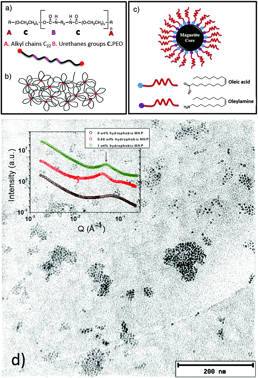 | ||
| Fig. 1 Sketch of the investigated system (a) HEUR polymer structure with long alkyl chain ends (A), urethane groups (B), and PEO groups (C), (b) HEUR polymer network in water (φ > 10 wt%), (c) core–shell magnetite nanoparticles with oleic acid and oleylamine coating and (d) transmission electron microscopy image of the nanocomposite with 1 wt% MNPs in the dry state. The inset shows the SANS curves of the nanocomposite gels, where the correlation peak resembles the domain spacing of the polymer network and the distance between the MNP clusters. | ||
We focused on the determination of the influence of the MNP on the repeat distance, i.e. the distance between the hydrophobic domains in the polymer network, revealing that, with increasing MNP concentration, the repeat distance also increases. When the MNPs are added to the HEUR hydrogel clusters of MNPs are also formed. In Fig. 1(d) a TEM image of the nanocomposite with 1 wt% MNPs is shown, and the MNP clusters are well visible. In the inset, the SANS profiles of the nanocomposites as hydrogels are shown with increasing MNP concentration (from ϕMNP = 0 wt% up to ϕMNP = 1 wt%) showing the correlation peak associated with the repeat distance at q ∼ 0.062 Å−1.
In this work, we investigate the dynamics of the same systems using two techniques: dielectric relaxation spectroscopy (DRS) and neutron spin echo (NSE) measurements. DRS allows us to measure the imaginary part of the permittivity ε′′, also called the dielectric loss, as a function of the frequency ω of the applied electric field, which is associated with the energy dissipation related to the dipole relaxations. The frequency range investigated by DRS is between 10−3 Hz and 106 Hz, therefore the investigated dynamics lies in the time range of milliseconds up to several seconds. On the other hand, NSE is a powerful tool to measure the coherent intermediate time-dependent scattering function, S(q,t), on the nanoseconds timescale (109 Hz) and on the nanometer length scale. Even though these two techniques probe different time-scales, they often probe the same type of dynamics,26,27 and can therefore complement each other in the study of the polymer dynamics.
2. Experimental
2.1 Materials
The telechelic polymer used for the polymer matrix is the so-called TAFIGEL® PUR 61 (25% water emulsion), Mw = 8900 g mol−1 (with Mw/Mn = 1.04) which was purchased from Münzing Chemie GmbH.For the MNP synthesis, iron(III) acetylacetonate (Fe(acac)3, 99.9%), 1,2-hexadecanediol (C14H29CH(OH)CH2(OH), 90%), oleylamine (OAM, C6H18![[double bond, length as m-dash]](https://www.rsc.org/images/entities/char_e001.gif) C9H17NH2, 70%), oleic acid (OA, C9H18C8H15COOH, 99%) phenyl ether (C12H10O, 99%), and solvents (hexane, ethanol) were purchased from Sigma Aldrich.
C9H17NH2, 70%), oleic acid (OA, C9H18C8H15COOH, 99%) phenyl ether (C12H10O, 99%), and solvents (hexane, ethanol) were purchased from Sigma Aldrich.
2.2 Hydrophobic magnetite nanoparticle synthesis
The coated magnetite nanoparticles were synthesized by a thermal decomposition of iron Fe(III) salt according to the procedure reported by Wang et al.28 Briefly, 0.71 g of Fe(acac)3 (2 mmol) was mixed in 20 mL of phenyl ether with 2 mL of oleic acid (6 mmol) and 2 mL of oleylamine (4 mmol) under a nitrogen atmosphere with vigorous magnetic stirring and 2.58 g (10 mmol) of 1,2-hexadecanediol was added into the solution. The solution was heated to 200 °C and refluxed for 2 h. After refluxing, the solution was cooled to room temperature and ethanol was added to it. The reaction product was separated by centrifuging using a Sigma 3K30 centrifuge at 10![[thin space (1/6-em)]](https://www.rsc.org/images/entities/char_2009.gif) 000 rpm for 20 minutes and redispersed in hexane in order to obtain a stock solution of magnetite nanoparticles (total Fe concentration: 3.6 ± 0.2 g L−1).
000 rpm for 20 minutes and redispersed in hexane in order to obtain a stock solution of magnetite nanoparticles (total Fe concentration: 3.6 ± 0.2 g L−1).
2.3 Hydrogel nanocomposite preparation
The nanocomposites in the hydrogel state were obtained by mixing 1 mL of telechelic polymer emulsion in D2O (25 wt%) and 0.42 mL of the 3.6 g L−1 stock solution of hydrophobic MNPs in order to achieve a hydrophobic MNP concentration of 0.46 wt% (with respect to the polymer mass) in the gel. We prepared the hydrogel with a concentration of hydrophobic MNPs of 0.80 wt% by adding 0.76 mL of the hydrophobic MNP solution (3.6 g L−1) to the telechelic polymer emulsion in D2O (25 wt%).2.4 Differential scanning calorimetry (DSC) measurements
Glass transition and crystallization/melting events were investigated in a nitrogen atmosphere in the temperature range from −160 to 100 °C using a TA Instruments Q200 series calorimeter. The samples were placed into aluminum pans (13.99 mg, 13.85 mg and 14.8 mg of the pure, with 0.46 wt% MNPs and with 0.80 wt% MNP films, respectively). Cooling and heating rates were fixed at 20 K min−1.2.5 Dielectric relaxation spectroscopy (DRS) measurements
Three HEUR hydrogels 25 wt% (aq) differing in MNP content (0 wt%, 0.46 wt% and 0.80 wt%) were investigated by DRS. A few mg of each sample were placed between the gold plated electrodes (diameter 20 mm) of a liquid sample cell BDS1308. Silica spacers with a diameter of 0.5 mm were used for electric isolation and control of the sample thickness. The resulting parallel plate capacitor was mounted in a cryostat and its temperature was controlled by a heated gas stream of nitrogen evaporated from the liquid state using a Novocontrol Quatro with an uncertainty of 0.1 °C. The dielectric function ε*(ω) = ε′(ω) − iε′′(ω) was then recorded using a Novocontrol Alpha Analyzer as a function of frequency in the range of 0.01 Hz–1 MHz. The temperature was varied from 25 °C to −100 °C in cooling steps of 5 °C or 10 °C.2.6 Neutron spin echo (NSE) measurements
NSE measurements were performed on the pure HEUR hydrogels 25 wt% (aq) and on the hydrogels containing MNPs. In order to achieve maximum contrast and minimum incoherent background arising from the protonated material, we used heavy water (D2O) as a solvent for the hydrogel samples. The measurements were performed using a J-NSE spectrometer in the FRMII research reactor in Garching, Germany,29 in the q-range between 0.05 Å−1 and 0.21 Å−1 at a wavelength of 8 Å probing Fourier times up to 40 ns. The samples were mounted in a thermostat controlled sample environment at 25 °C.3. Results and discussion
3.1 Differential scanning calorimetry analysis of the nanocomposite HEUR-MNP hydrogels
The DSC heating curve of the pure HEUR hydrogels 25 wt% (aq) is shown in Fig. 2(a). Starting from −160 °C, we observe the glass transition temperature (Tg) step which is enlarged in the inset in Fig. 2(a). The glass transition of the PEO portion of the HEUR polymer is observed for all nanocomposites as seen in Fig. 2(b). With increasing MNP concentration, the Tg of the polymer slightly decreases from ∼−78 °C to ∼−83 °C, i.e. by few degrees. At higher temperatures, we observe an exothermic peak at −48 °C, which can be attributed to the cold crystallization of water.30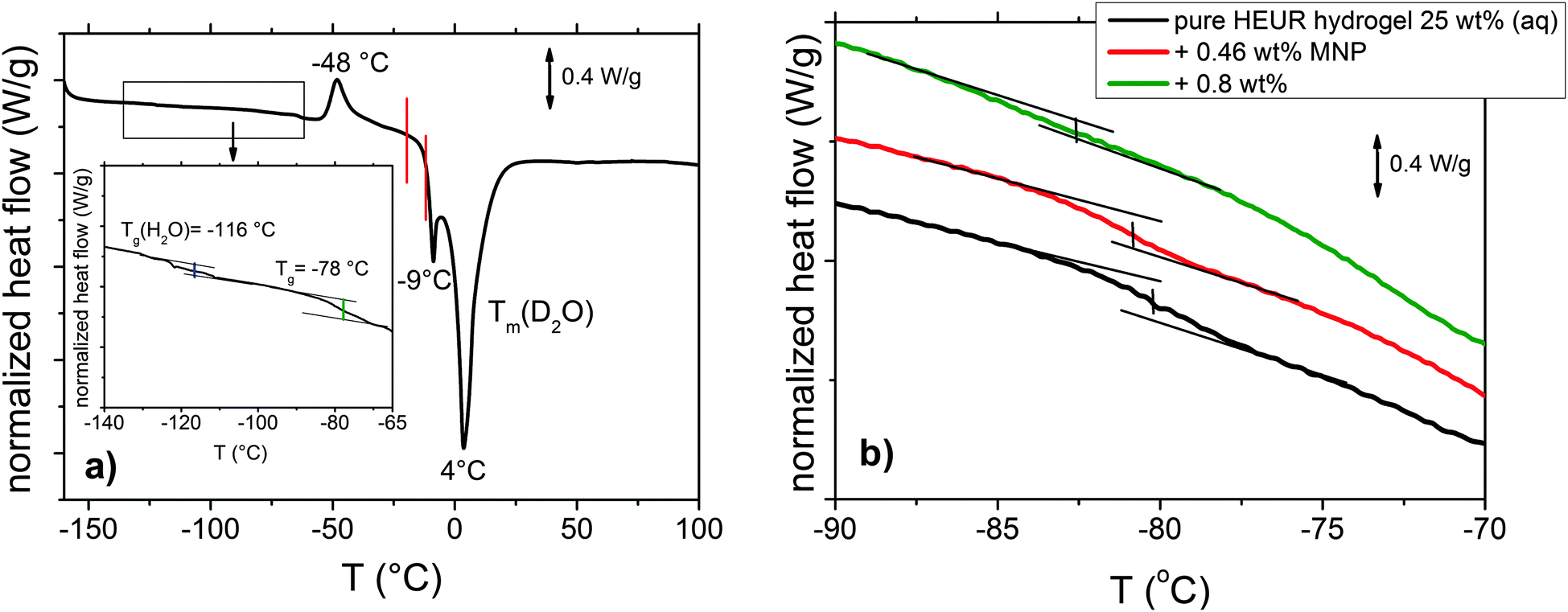 | ||
| Fig. 2 (a) DSC curve of the pure HEUR hydrogel 25 wt% (aq). For clarity, since we observed the same phase transitions for all the samples, we show only the curve of the “matrix” (the DSC curves of the nanocomposites are shown in Fig. S1 of the ESI†). In the inset, the glass transition temperatures Tg are highlighted in blue and green. The phase transition observed in the dielectric loss data is marked in red. (b) Enlarged region in the glass transition temperature range for the all composite samples with increasing MNP concentration. | ||
The cold crystallization process was found in several kinds of polymer–water systems investigated by DSC, e.g. polysaccharide–water systems.31,32 It occurs typically when the material is cooled sufficiently fast, such that the crystallization dynamics is arrested before the phenomenon is completed during cooling. When mobility is regained during the subsequent heating, the crystallization process continues and gives an exothermic event. In particular, for the poly(ethylene glycol) (PEG)–water system, which is similar to ours, it was found that the cold crystallization of the water for a system containing ∼60 wt% of H2O occurs at around −45 °C,16 which is in good agreement with the one we observe at −48 °C. At ∼4 °C, a deep endotherm occurs, accompanied by a shallower peak at −9 °C. They can be attributed to the melting of D2O in the hydrogel. Please note that the heavy water (D2O) used is expected to have a higher melting point than normal water.31,33 Also in previous calorimetric studies on polymer membranes containing water, a “double” endotherm peak assigned to the melting of the water was found.32,34 The peak at lower temperature was attributed to the melting of water clusters bound to the polymer, while the second one at higher temperature was associated with the “free” water molecules i.e. those which are not directly bound to the polymer. It was found that in a poly(HEMA) hydrogel, the state of the water can be divided into three categories: interfacial, bound and bulk water.35 The latter one crystallizes to ice and probably gives rise to the deep endotherm at 4 °C. The first two types supercool without crystallizing, remaining in the amorphous state, which is reflected by the presence of a glass transition. According to Pathnathan and Johari, the Tg of the supercooled water lies at −138.2 °C35 and, according to Cerveny, at −113–115 °C for bulk water and about −100 °C for confined water (depending on the confining system).36 In our case, we can observe it as a very weak step at −116 °C, highlighted in blue in the inset in Fig. 2(a).
3.2 Dielectric relaxation spectroscopy (DRS) analysis
The dielectric loss spectra recorded for the pure HEUR gel with 25 wt% (aq) are shown in Fig. 3 at the selected temperatures. At −95 °C a prominent dielectric loss peak occurs at ωmax ∼ 100 Hz for the pure HEUR hydrogel. Similar intense dielectric loss peaks have previously been found in other water containing systems, i.e. hydrogels,35 protein solutions,37 and hydrated PEO, where they were associated with the non-freezable water tightly bound to non-crystalline PEO segments.38 Similar peaks were observed also in the dielectric relaxation spectra of ice.39–41 According to Pathnathan and Johari, it is attributed to the thermally activated diffusion of molecules in supercooled water, which is identified as its α-relaxation process, and the relaxation peak is observed at 1 kHz at a temperature of −95 °C.35 As observed in Fig. 3 (black curve, indicated by a black arrow) and in Fig. 5, in addition to the main relaxation peak and partially hidden by it, there is a shoulder at ωmax ∼ 3 Hz. In the same frequency-temperature range a relaxation peak was found for the poly(HEMA) hydrogel35 and was attributed to the breaking and reforming of the H-bonds in the polymer network, defined as the β-process. With increasing temperature, the contribution of the conductivity becomes visible, leading to a “shoulder” at low frequency, i.e. ωmax ∼ 0.1 Hz, (see Fig. 3). Nevertheless, an additional relaxation can be detected at low frequencies (ωmax ∼ 1 Hz) concealed to a large extent by the conductivity slope at low frequencies. Upon further increasing the temperature up to T = −10 °C we observe a drastic change of the dielectric loss profiles which become flat in the low frequency range (0.01 Hz < ωmax < 1 Hz) and do not show any relaxation peaks in the higher frequency range, i.e. 10 Hz < ωmax < 105 Hz (note that the curves at T = −10 °C, T = −5 °C and T = 20 °C superimpose in Fig. 3).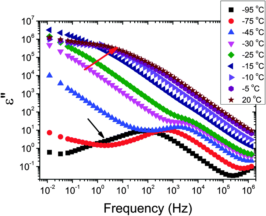 | ||
| Fig. 3 Dielectric loss data of the pure HEUR hydrogel with 25 wt% (aq) in the temperature range between −95 °C and 20 °C. For clarity, only the curve at temperatures where significant changes in the DRS data occur is shown. The black arrow indicates the shoulder at ∼3 Hz at −95 °C, and the red one indicates the flat profile of the DRS data in the low frequency range. | ||
In order to follow more closely the temperature evolution of the relaxation, we plot the ε′′ values at selected fixed frequencies, as a function of temperature, which are shown for the pure hydrogel in Fig. 4. The step at ∼−15 °C highlighted in Fig. 4 by a dashed line does not shift with frequency, meaning that in that temperature range a phase transition in the sample occurs. Looking at the DSC curve in Fig. 2(a), we observe that this temperature corresponds to the onset of the water melting (indicated by red lines in Fig. 2(a)). This means that the water melting in the gel is reflected in the dielectric loss spectra as a steep increase of the conductivity, as indicated by the high value of ε′′ (∼106) at low frequencies (ωmax ∼ 1 Hz) (indicated by the green arrow in Fig. 4). The high values of ε′ (∼106) (Fig. S2 of the ESI†) at low frequencies at temperatures above −25 °C are a sign of the electrode polarization process.42 Therefore, the dielectric data between −25 °C and 25 °C will not be discussed in detail here. By comparing the dielectric loss data of the pure HEUR hydrogel with the ones containing MNPs, as done in Fig. 5, it is possible to observe the influence of the MNP on the dielectric loss profile.
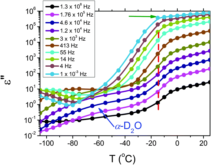 | ||
| Fig. 4 Isochronal plot of the pure HEUR hydrogel 25 wt% (aq). The red dashed line indicates the position of the step at ∼15 °C, indicating the phase transition observed in the DSC data. | ||
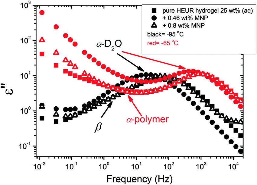 | ||
| Fig. 5 Dielectric loss data at −95 °C (black symbols) and at −65 °C (red symbols) for all the investigated composites and the pure HEUR hydrogel. The black arrows indicate the β-process and the α-process related to D2O at −95 °C. The red arrows indicate the α-process of the polymer and the α-process related to D2O at −65 °C. | ||
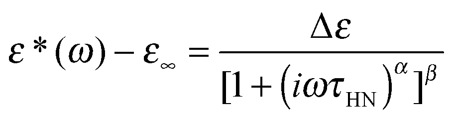
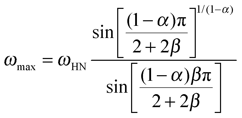
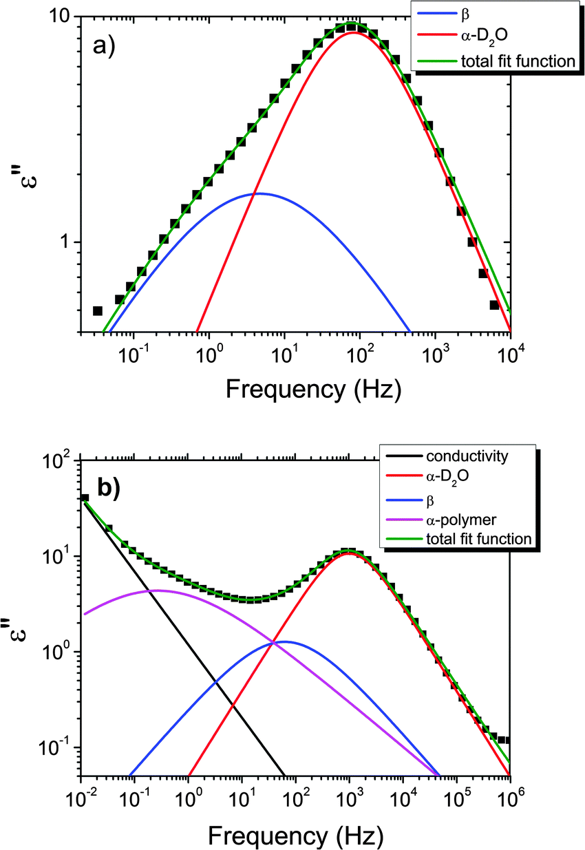
We now focus on the effect of the MNPs on the α-relaxation of water. This relaxation is visible in a rather wide temperature range. In Fig. 5, the corresponding ε′′ peak is shown at two temperatures namely −95 °C and −65 °C. Interestingly, for the pure HEUR hydrogel and the hydrogel with 0.80 wt% MNP content, we observe only a very weak shoulder at ωmax ∼ 3 Hz (indicated by an arrow marked β in Fig. 5) at T = −95 °C. This peak is attributed to the β-process. According to the frequency-temperature range, to the assignment done by Pathnathan and Johari for poly(HEMA) hydrogels35 and to the relaxation process found by Huh and Cooper in polyurethane block polymers,43 this process is related to the motion of the dipolar segments –OH and –CO along the C–O axis. The most prominent peak at −95 °C occurring at ωmax ∼ 100 Hz for the pure HEUR hydrogel and the one with 0.80 wt% MNP content is shifted to ωmax ∼ 20 Hz for the HEUR hydrogel with 0.46 wt% MNPs. A similar shift is also observed at −65 °C. This shift is not well understood. In order to quantify our results in terms of time scales as a function of temperature, we performed a fitting procedure. The dielectric loss data were fitted by a sum of Havriliak–Negami (HN) model function terms of the form:
 | (1) |
 | (2) |
| τ = τ0eB/(T−T0) | (3) |
| τ = τ0eEA/RT | (4) |
O along the C–O axis, namely the β-process. In our system, because of the presence of water, H-bonds are present between the water molecules and the hydroxyl (–OH) and carbonyl (–CO) groups of the polymer chains. Thus, the activation energy of the β-process is determined by the breaking and reforming of the H-bonds in the hydrogel network. As seen in Table 1, the activation energy EA decreases with increasing MNP content. This means that the rotation of the –OH and –CO groups becomes “easier” in terms of energy barrier. This effect might be explained considering the blob model adopted for star polymers by Halperin.46 According to this model, the polymer chain can be described in terms of “blobs’’, i.e. spherical regions occupied by segments of the polymer chain. The polymer concentration is higher nearby the branch point of the star polymer, which, in our case, is replaced by the hydrophobic domain. When the MNPs are added to the hydrogels, they interact mainly with the hydrophobic domains, being embedded into them. The increase of the hydrophobic domain size, due to the presence of the MNP clusters, leads to a “dilution” of the polymer concentration nearby the “branching point”. Therefore, the “blobs” feel less constrains, and as a consequence also the rotation of the polar groups –OH and CO becomes easier. The activation energies EA of the β-process are shown in Table 1.
 | ||
| Fig. 6 Example of the fitting of the dielectric loss data of the pure HEUR gel 25 wt% (aq) at (a) −100 °C and at (b) −65 °C. Details are explained in the text. | ||
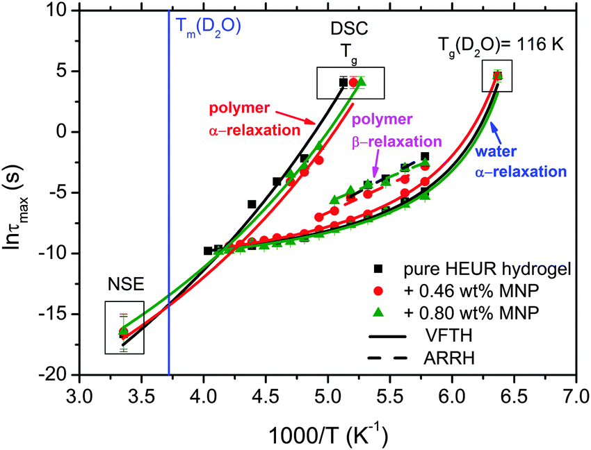 | ||
| Fig. 7 Arrhenius map showing: the α-process related to the polymer chain including the NSE relaxation time at q = 0.05 Å−1 and the relaxation time at the Tg (100 s) (the green arrow indicates the increase of the curvature at 0.80 wt% MNPs), and the β-process and the α-process related to the supercooled water (α-water). The lines are VFTH fits and the dashed ones are Arrhenius fits. The vertical blue line indicates the melting of D2O detected by DSC. | ||
| Sample | T g,diel (α-D2O) (°C) | T g (α-D2O) (°C) | T g (α-polymer) (°C) (DSC) | E A (β) (kJ mol−1) |
|---|---|---|---|---|
| Pure HEUR hydrogel | −119.3 ± 2.3 | −116 | −78 | 45.5 ± 1.8 |
| +0.46 wt% MNPs | −115.1 ± 2.2 | −116 | −81 | 39.2 ± 2.4 |
| +0.80 wt% MNPs | −124.5 ± 5.2 | −116 | −84 | 34.6 ± 3.2 |
With increasing temperature, we observe an additional process in the temperature range between −70 °C and −50 °C for the hydrogels with 0.46 wt% and 0.80 wt% MNP content, and between −65 °C and −35 °C for the pure HEUR hydrogel (25 wt% (aq)), which is partially hidden by the conductivity and the α-water process. It is shown in one fit example in Fig. 6(b) (magenta curve). The relaxation time was measurable only at three temperatures and therefore it is not clear whether its trace in the activation plot (Fig. 7) is an Arrhenius or a VFTH one. Note however, that assuming a VFTH behavior, it corresponds well to the points related to the glass transition of the polymer as observed by DSC. Hence, we assign it to the α-relaxation of the HEUR polymer, in particular to the PEO portion of the polymer chain.47,48 Further evidence for this assignment will be given upon the presentation of the results regarding segmental dynamics as observed by neutron spin echo. For the time being, we would like to point out that DSC shows a systematic acceleration of dynamics with MNP content (decrease of Tg) while DRS shows that the higher loading nanocomposite has slightly faster dynamics than its low loading counterpart. We will come back to this point later. By extrapolating the fitted VTFH lines to the time τ = 100 s, we get a measure of the glass transition temperature related to the supercooled water, namely the dielectric glass transition temperature Tg,diel. The obtained values are shown in Table 1. These values are in agreement with the experimental Tg values obtained by DSC.
The observed decrease of the Tg with increasing MNP concentration (Fig. 2(b)) indicates an acceleration of the dynamics at T ∼ Tg, therefore at long relaxation times τ. This fact can be related to the change of the curvatures of the VFTH traces (Fig. 7). This curvature is often expressed in terms of the fragility index, which is a measure of the cooperativity of the dynamics, which reads:
 | (5) |
3.3 Conductivity data
In order gain insights into the correlation between the charge transport mechanism and the segmental relaxation (α-relaxation), the conductivity data collected in the DRS experiments turn to be useful. In Fig. 8, the real part of the conductivity σ′ is plotted as a function of frequency at −55 °C. The plateau in the conductivity at ∼10−1 Hz increases when MNPs are added to the pure HEUR hydrogel. However, for the intermediate MNP concentration (0.46 wt%), the plateau is higher than that for the composite having the highest MNP concentration (0.80 wt%). This suggests that the difference in the conductivity might be related to the difference in the polymer mobility (i.e. segmental motion) and not exclusively to the conductive nature of the MNPs.50 Indeed, according to the classical theory51 ionic conductivity in a polymer is inversely proportional to its segmental relaxation time τα. This means that ion motions are possible only when polymer segments undergo large amplitude rearrangements. In order to test this relation we compare the α-relaxation process and the conductivity of all samples. We plot the plateau value of σ′ as a function of the relaxation times of the α-relaxation, τα, for all samples (Fig. 9). The lines of the pure HEUR hydrogel and the nanocomposites do not coincide, meaning that a different relationship subsists between the conductivity and the α-relaxation for the pure hydrogel and for the nanocomposites. On the other hand, the traces of the nanocomposite gels in Fig. 9 coincide. This means that the α-relaxation of the polymer and the conductivity of the nanocomposites are directly coupled and they can be compared. Therefore, we can attribute the decrease of the conductivity observed for the nanocomposite with 0.80 wt% MNPs to a decrease of the segmental mobility of the polymer.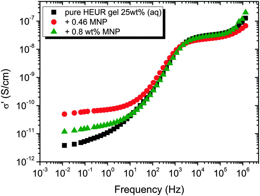 | ||
| Fig. 8 Real part of the conductivity, σ′ (S cm−1), as a function of the frequency at −55 °C for the HEUR gels (25 wt% (aq)) for increasing MNP concentration. | ||
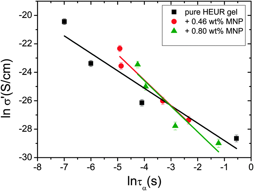 | ||
| Fig. 9 Double logarithmic plot of the real part of the conductivity, σ′ (S cm−1), as a function of the relaxation times of the α-process, τα (s), for all the investigated gels. | ||
3.4 Neutron spin echo (NSE) measurements
In the NSE experiments the intermediate scattering function S(q,t), which is the Fourier transform of the spectral function S(q,ω), is measured. In terms of the atomic coordinate expression, it reads like: | (6) |
 | (7) |
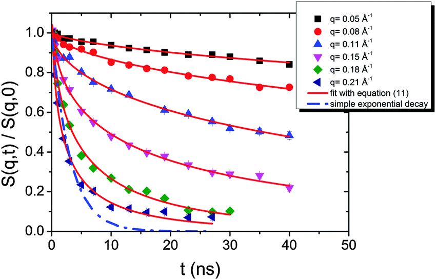 | ||
| Fig. 10 Intermediate scattering functions of the pure HEUR hydrogel 25 wt% (aq). The red lines are the fitting curves (eqn (11)) while the dashed line represents a simple exponential decay at q = 0.21 Å−1. | ||
The intermediate scattering functions of the pure HEUR hydrogel (25 wt% (aq)) decay exponentially with time in the q range between 0.05 Å−1 and 0.15 Å−1, while for q = 0.18 Å−1 and q = 0.21 Å−1 they do not decay exponentially for longer Fourier times, as seen when comparing the data with a simple exponential decay (dashed line in Fig. 10).
The same result is found for the HEUR hydrogels containing MNPs (data shown in Fig. S3 of the ESI†). For a better understanding the intermediate scattering functions at q = 0.21 Å−1 are compared in Fig. 11 for all investigated samples. It is observed that the time decay is slightly slowed down for the hydrogel with 0.80 wt% MNPs, i.e. the intermediate scattering function tends to zero more slowly than the one of the pure HEUR hydrogel with 25 wt% (aq). Detailed differences in the dynamic processes occurring in the investigated hydrogels in the nanosecond time-scale can be investigated by fitting the intermediate scattering function with an appropriate dynamic model.
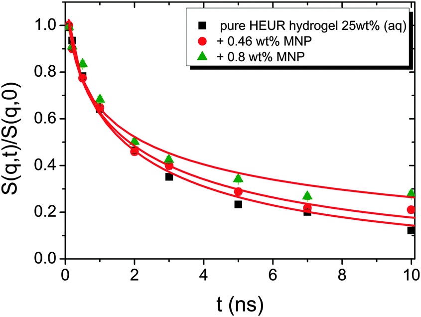 | ||
| Fig. 11 Intermediate scattering functions of the pure HEUR hydrogel 25 wt% (aq) (black squares), with 0.46 wt% MNP content (red circles) and with 0.80 wt% MNP content (green triangles) in the time range between 0 and 10 ns at q = 0.21 Å−1. | ||
From Fig. 10, it is possible to observe that the intermediate scattering functions for q > 0.08 Å−1 clearly decay exponentially up to Fourier times of t ∼ 20 ns. In contrast, for longer Fourier times the decay is strongly delayed, and at q = 0.18 Å−1 and q = 0.21 Å−1. The origin of this effect arises from the gel structure. In fact, the dynamics probed by NSE is dominated by the segmental mobility of the polymer chain. However, in a gel-like network, cross-links and entanglements constrain the local segmental mobility of the chain, leading to a non-decaying intermediate scattering function. The scattering from these inhomogeneities such as crosslinks, entanglements and regions with different polymer densities gives an elastic contribution to the intermediate scattering function. This contribution was generally observed in polymer gels52 and in our previous SANS investigation on the HEUR hydrogels with embedded MNPs20 as an excess scattering, i.e. very high scattering intensity in the low-q region of I(q).53 According to earlier studies on the mesoscopic structure of charged gels,52 the scattering intensity in the low q-region of highly concentrated gels arises from solid-like density fluctuations, coming from an inhomogeneous distribution of crosslinks of the polymer network.53 The scattering from these so-called “static inhomogeneities” can be described by an additional term included in the scattering function, which, according to the Debye–Bueche formalism, reads:54
 | (8) |
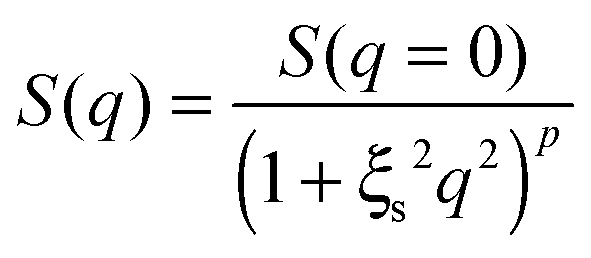
According to our scenario, this extra-scattering term arising from the static inhomogeneity was taken into account in the intermediate scattering function expression, in terms of a fraction of a non-decaying component P(q). Therefore, the intermediate scattering function expression reads:
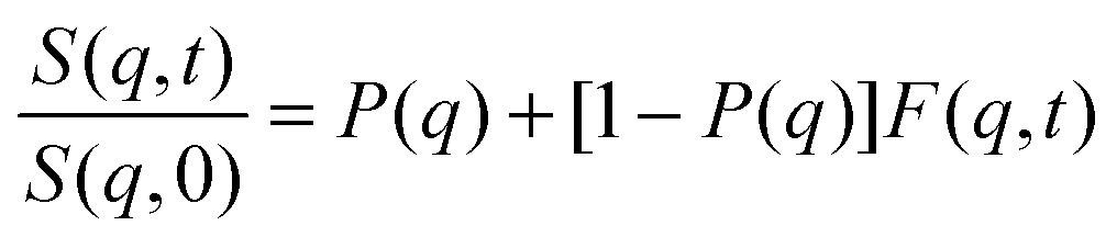 | (9) |
The generalized decay function F(q,t) shown in eqn (9) is generally expressed in terms of the long-time behavior of the normalized intermediate scattering function, which is approximately described by the so-called stretched exponential function:
| F(q,t) ∼ exp[−(Γt)β] | (10) |
In the case of the investigated HEUR hydrogels, the intermediate scattering functions shown in Fig. 10 are well fitted using the Zimm model for the segmental dynamics of polymers in solution. It describes the dynamics of a Gaussian chain in terms of a bead spring model, and includes the hydrodynamic interaction between the chain segments.55 In particular, since we observed a time-decay up to Fourier-times of t ∼ 20 ns we used the limit of the short-time scale of the Zimm model, with β = 0.85.56,57 Therefore, taking into account the contribution of the “static inhomogeneities” to the intermediate scattering function time-decay, the total expression of the intermediate scattering function used to fit our data reads:
 | (11) |
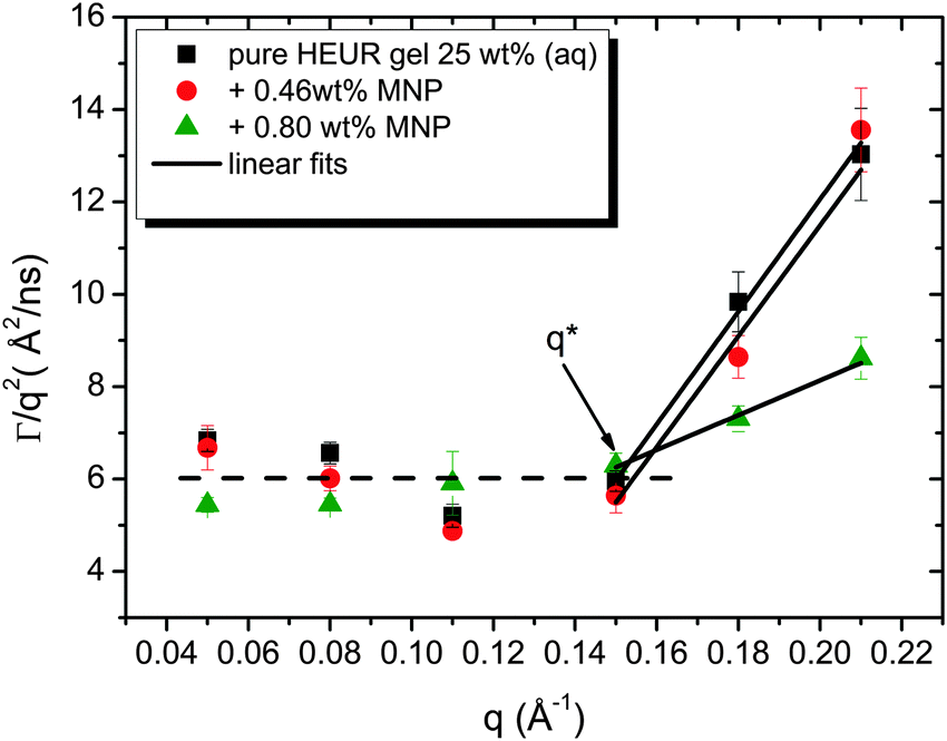 | ||
| Fig. 12 Diffusion coefficients Γ/q2 of the pure HEUR hydrogel (black squares), with 0.46 wt% MNPs (red circles) and with 0.80 wt% MNPs as a function of the q vector. The black lines are linear fits. q* indicates the crossover between the simple diffusion and the segmental dynamics regimes. | ||
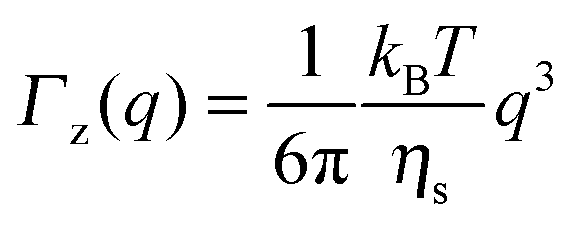
As observed from the plot in Fig. 12, all investigated hydrogels exhibit two regimes: a diffusive region where Γ ∝ q2 in the q range between 0.05 Å−1 and 0.11 Å−1 where the diffusion coefficient is a constant and a Zimm-like internal dynamic regime where Γ ∝ q3, in the q range between 0.15 Å−1 and 0.21 Å−1.58 Indeed, the relaxation rate ΓZ calculated in the Zimm model is given by:
 | (12) |
 | (13) |
 | (14) |
Indeed, the total scattering intensity of a gel measured by SANS is given as an incoherent sum of the scattering from the static inhomogeneities, Sst(q) and the scattering due to the thermal concentration fluctuations Sth(q) in the gel61,62
| S(q) = Sst(q) + Sth(q) | (15) |
| Sst(q) = P(q) × S(q) | (16) |
 | (17) |
 | ||
| Fig. 13 SANS intensities of (a) the pure HEUR hydrogel and (b) the one containing 0.46 wt% MNPs. The green points represent the static scattering contribution Sst(q) to the total scattering intensity S(q) (black squares). The red lines represent the Teubner–Strey fits. | ||
We focus now on the pure HEUR hydrogel, and analyze the correlation length calculated from the bare SANS intensities and that of the deducted static scattering contribution. The correlation length determined in the analysis of the overall SANS scattering is ξSANS = (17.2 ± 0.3) Å whereas the correlation length of the frozen density fluctuations is ξNSE = (43 ± 5) Å. In turn, this means that the system comes to a more structured state by the relaxation process. This suggests that the static scattering contribution Sst(q) arises from a more ordered system than the one which gives the total scattering intensity S(q), and it is therefore characterized by a longer correlation length ξNSE. The TS fits on the main correlation peak at qmax ∼ 0.062 Å−1 cannot be performed for the static scattering contribution of the hydrogels containing MNPs, due to the interference of the second correlation peak of S(q) at q = 0.1 Å−1 arising from the MNP clusters (Fig. 13(b)). This means that for the HEUR hydrogels containing MNPs, the MNP clusters contribute to the “frozen” inhomogeneities which cause the retardation in the time decay of the intermediate scattering function.
3.5 Comparison between the DRS and NSE results on the polymer segmental relaxation
The neutron spin echo (NSE) and the dielectric relaxation spectroscopy (DRS) probe the same type of dynamics, although at different time scales. Therefore it is should be possible to compare the NSE and the DRS results on the segmental dynamics of the HEUR polymer for all the investigated hydrogels. The NSE results are summarized in Fig. 12, where the relaxation rate is plotted as a function of q2. At q > 0.15 Å−1 we observe a decrease of the relaxation rate Γ for the sample with 0.80 wt% MNP concentration compared to the pure HEUR hydrogel. This we addressed to the change of the biggest blob size in the system upon adding considerable MNPs to the system.From the activation energies of the beta relaxation (Arrhenius, Fig. 7 and Table 1) we see the similar trend of changing blob sizes – just from the smallest blobs that act on the polymer segments in terms of differing monomer density. So the evidence of the blob field as a function of MNP concentration is given.
Quite astonishing was the conductivity, which increased strongly for the middle concentration of MNP, and dropped down for the highest MNP concentration. Apart from the blob interpretation we saw initial trends of interpretation from the conductivity/relaxation time plot (Fig. 9) that displayed different mechanisms for the system without and with MNPs. Following this plot (Fig. 9) on the fast relaxation times, and reading the relaxation times from the NSE data at higher Q (Fig. 12), one would expect two steps: from 0 to 0.46% MNPs the relaxation time does not change, but the mechanism of conductivity changes, which leads to a considerable increase of conductivity. From 0.46% to 0.80% of MNP, the relaxation time increases, but the mechanism is identical, which leads to a moderately decreased conductivity. So, two competing trends finally can explain the conductivity dependence of our system.
4. Summary and conclusions
The dynamics of nanocomposite hydrogels composed of HEUR polymers and MNPs was investigated by DRS and NSE. From the DRS results, we detected three relaxation processes in the temperature range between −100 °C and −25 °C:(1) The so-called α-water relaxation, associated with the glass transition of the super-cooled water inside the hydrogels. This relaxation is not affected by the MNPs. We have extracted the glass transition of the super-cooled water, listed in Table 1.
(2) The segmental polymer relaxation, the α-relaxation, related to the glass transition of the polymer. In calorimetry, we observe that the Tg is decreased by ∼4 °C with increasing MNP concentration (values of the Tg shown in Table 1), indicating an acceleration of the segmental dynamics at long time scales (τ ∼ 100 s).
(3) The β-relaxation, which we relate to the rotation of dipolar segments like CO and O–H, forming H-bonds with the water. We observe a decrease of the activation energy EA associated with this process, with increasing MNP concentration. This result suggests that the MNP clusters lead to an increase of the sizes of the hydrophobic domains, which results in a dilution of the polymer blobs near the hydrophobic domain. As a consequence, the mobility of the smallest blobs is higher. In contrast, the smallest blobs of the pure HEUR hydrogel freeze stepwise at low temperatures and effectively shorten the mobile connecting arms. This results in a more mobile network with suppressed collective motions.
In general, thanks to three different techniques, i.e. DSC, DRS and NSE, we can observe the different effects of the MNPs on the segmental dynamics of the polymer at different time and length scales. In particular, we observed:
(i) At long time scales (τ ∼ 100 s), probed by DSC: an acceleration of the segmental dynamics.
(ii) At intermediate time scales (τ ∼ 10 ms), probed by DRS: cross-over region, where the α-relaxation times of the different nanocomposites overlap.
(iii) At short time scales (τ ∼ 10 ns), probed by NSE: a deceleration of the segmental dynamics.
We explain this difference with the change of the curvature of VFTH traces, which is related to the cooperativity of the α-relaxation. We find an increase of the cooperativity with increasing MNP concentration. Therefore, the present systems qualify as absorbers for electromagnetic fields,10 since decreased energies or slowing down facilitates the energy dissipation. The addition of MNPs is a way to decrease the glass transition of the polymer, and therefore to modify the viscoelastic properties of the material.
Magnetic relaxation measurements could be an interesting investigation for the HEUR-MNP hydrogel systems, since they would give information about the relaxation of the dispersed nanoparticles and allow to distinguish between physically trapped and mobile nanoparticles.68 Moreover, NSE measurements carried out in paramagnetic mode would be of some interest in order to have additional insights into the dynamics of the MNP.69 However, both types of measurements are beyond the scope of the present study.
Acknowledgements
Prof. Müller-Buschbaum acknowledges financial support from the International Research Training Groups 2022 Alberta/Technical University of Munich International Graduate School for Environmentally Responsible Functional Hybrid Materials (ATUMS). We thank Prof. Hiroshi Watanabe (ICR Kyoto University) for the helpful discussion about the DRS data. We also thank Dr Ana Rita Brás (Department Chemie, Universität zu Köln, Germany) for the experimental support in performing the DRS measurements.Notes and references
- P. Schexnailder and G. Schmidt, Colloid Polym. Sci., 2009, 287, 1–11 CAS.
- P. M. XuLu, G. Filipscei and M. Zrinyl, Macromolecules, 2000, 33, 1716–1719 CrossRef CAS.
- B. Luo, X.-J. Song, F. Zhang, A. Xia, W.-L. Yang, J.-H. Hu and C.-C. Wang, Langmuir, 2010, 26(3), 1674–1679 CrossRef CAS PubMed.
- C. Paquet, H. W. de Haan, D. M. Leek, H.-Y. Lin, B. Xiang, G. Tian, A. Kell and B. Simard, ACS Nano, 2011, 5(4), 3104–3112 CrossRef CAS PubMed.
- N. Zhang, J. Lock, A. Sallee and H. Liu, ACS Appl. Mater. Interfaces, 2015, 7(37), 20987–20998 CAS.
- Y. Yao, E. Metwalli, B. Su, V. Körstgens, D. Moseguí González, A. Miasnikova, A. Laschewsky, M. Opel, G. Santoro, S. V. Roth and P. Müller-Buschbaum, ACS Appl. Mater. Interfaces, 2015, 7, 13080–13091 CAS.
- S. Kurzhals, R. Zirbs and E. Reimhult, ACS Appl. Mater. Interfaces, 2015, 7(34), 19342–19352 CAS.
- C. J. Sunderland, M. Steiert, J. E. Talmadge, A. M. Derfus and S. E. Barry, Drug Dev. Res., 2006, 67, 70–93 CrossRef CAS.
- R. V. Ramanujan and L. L. Lao, Smart Mater. Struct., 2006, 15, 952–956 CrossRef.
- V. B. Bregar, IEEE Trans. Magn., 2004, 40(3), 1679–1684 CrossRef CAS.
- Y. Zhang, C. Pilapong, Y. Guo, Z. Ling, O. Cespedes, P. Quirke and D. Zhou, Anal. Chem., 2013, 85(19), 9238–9244 CrossRef CAS PubMed.
- S. B. Darling, N. A. Yufa, A. L. Cisse, S. D. Bader and S. J. Sibener, Adv. Mater., 2005, 17, 2446–2450 CrossRef CAS.
- S. B. Darling and S. D. Bader, J. Mater. Chem., 2005, 15, 4189–4195 RSC.
- C.-T. Lo and W. T. Lin, J. Phys. Chem. B, 2013, 117, 5261–5270 CrossRef CAS PubMed.
- V. Lauter-Pasyuk, H. Lauter, D. Ausserre, Y. Gallot, V. Cabuil, E. Kornilov and B. Hamdoun, Phys. B, 1998, 241–243, 1092–1094 Search PubMed.
- Y. Yao, E. Metwalli, J. F. Moulin, B. Su, M. Opel and P. Müller-Buschbaum, ACS Appl. Mater. Interfaces, 2014, 6, 18152–18162 CAS.
- M. M. Abul Kashem, J. Perlich, A. Diethert, W. Wang, M. Memesa, J. S. Gutmann, E. Majkova, I. C. Capek, S. V. Roth, W. Petry and P. Müller-Buschbaum, Macromolecules, 2009, 42, 6202–6208 CrossRef CAS.
- M. M. Abul Kashem, J. Perlich, L. Schulz, S. Roth, W. Petry and P. Müller-Buschbaum, Macromolecules, 2007, 40, 5075–5083 CrossRef.
- Y. Yao, E. Metwalli, M. A. Niedermeier, M. Opel, C. Lin, J. Ning, J. Perlich, S. V. Roth and P. Müller-Buschbaum, ACS Appl. Mater. Interfaces, 2014, 6, 5244–5254 CAS.
- A. Campanella, Z. Di, A. Luchini, L. Paduano, A. Klapper, M. Herlitschke, O. Petracic, M. S. Appavou, P. Müller-Buschbaum, H. Frielingaus and D. Richter, Polymer, 2015, 60, 176–185 CrossRef CAS.
- A. N. Semenov, J. F. Joanny and R. Khokhlov, Macromolecules, 1995, 28, 1066–1075 CrossRef CAS.
- A. N. Semenov, I. A. Nyrkova and M. E. Cates, Macromolecules, 1995, 28, 7879–7885 CrossRef CAS.
- K. W. Paeng, B.-S. Kim, E.-R. Kim and D. Sohn, Bull. Korean Chem. Soc., 2000, 21, 623–627 CAS.
- K. C. Tom, R. D. Jenkins, M. A. Winnik and D. R. Bassett, Macromolecules, 1998, 13, 4149–4159 CrossRef.
- S. Suzuki, T. Uneyama and H. Watanabe, Macromolecules, 2013, 46, 3497–3504 CrossRef CAS.
- D. Richter, A. Arbe, J. Colmenero, M. Monkenbusch, B. Farago and R. Faust, Macromolecules, 1998, 31, 1133 CrossRef CAS.
- A. Faivre, C. Levelut, D. Durand, S. Longeville and G. Ehlers, J. Non-Cryst. Solids, 2002, 712, 307–310 Search PubMed.
- L. Wang, J. Luo, Q. Fan, M. Suzuki, I. S. Suzuki, M. H. Engelhard, Y. Lin, N. Kim, J. Q. Wang and C. J. Zhong, J. Phys. Chem. B, 2005, 109, 21593–21601 CrossRef CAS PubMed.
- O. Holderer, M. Monkenbusch, R. Schätzler, H. Kleines, W. Westerhausen and D. Richter, Meas. Sci. Technol., 2008, 19, 034022 CrossRef.
- M. Tanaka, T. Motomura, I. Naoki, S. Kenichi, O. Makoto, M. Akira and H. Tatsuko, Polym. Int., 2000, 49, 1709–1713 CrossRef CAS.
- T. Hatakeymaa, H. Kasuga, M. Tanaka and H. Hatakeyamad, Thermochim. Acta, 2007, 465, 59–66 CrossRef.
- H. Yoshida, T. Hatakeyama and H. Hakateyama, Polymer, 1990, 31, 693–698 CrossRef CAS.
- P.G. Hill, R.D. MacMillan, V. Lee, INIS Report, 1981, 14.
- Shimadzu, 2015, Retrieved from http://www.shimadzu.com/an/industry/electronicselectronic/fc160306010.htm.
- K. Pathnathan and G. P. Johari, Colloid Polym. Sci., 1990, 28, 675–689 Search PubMed.
- S. Cerveny, G. A. Schwartz, R. Bergman and J. Swenson, Phys. Rev. Lett., 2004, 93, 245701 CrossRef PubMed.
- N. Shinyashiki, W. Yamamoto, A. Yokoyama and T. Yoshinari, J. Phys. Chem. B, 2009, 113, 14448–14456 CrossRef CAS PubMed.
- X. Jin, S. Zhang and J. Runt, Macromolecules, 2003, 36, 8033–8039 CrossRef CAS.
- R. P. Auty and R. H. Cole, J. Chem. Phys., 1957, 20, 1304–1309 Search PubMed.
- G. P. Johari and E. Whalley, J. Chem. Phys., 1981, 75, 1333–1340 CrossRef CAS.
- A. von Hippel, IEEE Trans. Electr. Insul., 1988, 231, 801–816 CrossRef.
- A. Serghei, M. Tress, J. R. Sangoro and F. Kremer, Phys. Rev. B: Condens. Matter Mater. Phys., 2009, 80, 184301 CrossRef.
- D. S. Huh and S. L. Cooper, Polym. Eng. Sci., 1971, 11, 369–375 CAS.
- F. Kremer, J. Non-Cryst. Solids, 2002, 305, 1–9 CrossRef CAS.
- E. J. Donth, Relaxation and Thermodynamics in Polymers: Glass Transition, Akademie-Verlag, Berlin, 1992 Search PubMed.
- A. Halperin, Macromolecules, 1987, 20, 2943–2946 CrossRef CAS.
- X. Jin, S. Zhang and J. Runt, Polymer, 2002, 43, 6247–6254 CrossRef CAS.
- J. J. Fontanella, M. C. Wintersgill, P. J. Welcher and J. P. Calame, IEEE Trans. Electr. Insul., 1985, 6, 943–946 CrossRef.
- R. Böhmer, K. L. Ngai, C. A. Angell and D. J. Plazek, J. Chem. Phys., 1993, 99, 4201–4209 CrossRef.
- A. Killis, J. LeNest, H. Cheradame and A. Gandini, Makromol. Chem., 1982, 183, 2835 CrossRef CAS.
- M. A. Ratner and D. F. Shriver, Chem. Rev., 1988, 88, 109 CrossRef CAS.
- M. Sugiyama, M. Annaka, K. Hara, M. E. Vigild and G. D. Wignall, J. Phys. Chem. B, 2003, 107, 6300–6308 CrossRef CAS.
- A. M. Hecht, F. Horkay, P. Schleger and E. Geissler, Macromolecules, 2002, 35, 8552–8555 CrossRef CAS.
- P. Debye and A. M. Beuche, J. Appl. Phys., 1949, 20, 518–525 CrossRef CAS.
- M. Rubistein and R. H. Colby, Polymer Physics, Oxford University Press, New York, 2003 Search PubMed.
- B. Ewen and D. Richter, Neutron Spin Echo Investigations on the Segmental Dynamics of Polymers in Melts, Networks and Solutions, Advances in Polymer Science, Springer-Verlag, Berlin, 1987, pp. 1–129 Search PubMed.
- M. Doi and S. F. Edwards, The theory of polymer dynamics, International Series of Monographs on Physics, Oxford University Press, Oxford, 1994 Search PubMed.
- D. Richter, J. Colmenero, M. Monkenbusch and A. Arbe, Neutron Spin Echo in Polymer Systems, Advances in Polymer Science, Springer-Verlag, Berlin, Heidelberg, 2005, pp. 1–221 Search PubMed.
- L. Leibler, M. Rubinstein and R. H. Colby, Macromolecules, 1991, 24, 4701–4707 CrossRef CAS.
- T. Gregory Dewey, Fractals in Molecular Biophysics, Oxford University Press, New York, 1997 Search PubMed.
- S. Panyukov and Y. Rabin, Macromolecules, 1996, 29, 7960 CrossRef CAS.
- A. Onuki, J. Phys. II, 1992, 2, 45–61 CrossRef CAS.
- S. Koizumi, M. Monkenbusch, D. Richter, D. Schwahn and B. Farago, J. Chem. Phys., 2004, 12721–12731 CrossRef CAS PubMed.
- S. Koizumi, M. Monkenbusch, D. Richter, D. Schwahn, B. Farago and M. Annaka, J. Neutron Res., 2002, 10, 155–162 CrossRef CAS.
- S. Koizumi, M. Monkenbusch, D. Richter, D. Schwahn and M. Annaka, J. Phys. Soc. Jpn. Suppl. A, 2001, 320 Search PubMed.
- C. Frank, H. Frielinghaus and J. Allgaier, Langmuir, 2007, 23, 6526–6535 CrossRef CAS PubMed.
- M. Teubner and R. Strey, J. Chem. Phys., 1987, 87, 3195–3200 CrossRef CAS.
- R. Kötitz, W. L. Trahms, W. Brewer and W. Semmler, J. Magn. Magn. Mater., 1999, 194, 62–68 CrossRef.
- H. Casalta, P. Schleger, C. Bellouard, M. Hennion, I. Mirebeau, G. Ehlers, B. Farago, J. L. Dorman, M. Kelsch, M. Linde and F. Phillipp, Phys. Rev. Lett., 1999, 82, 1301–1304 CrossRef CAS.
Footnote |
| † Electronic supplementary information (ESI) available. See DOI: 10.1039/c6sm00074f |
| This journal is © The Royal Society of Chemistry 2016 |