Absolute isotope ratios of carbon dioxide – a feasibility study†
Received
10th July 2020
, Accepted 19th August 2020
First published on 9th September 2020
Abstract
One way of obtaining isotope ratios, traceable to the International System of Units, is the gravimetric isotope mixtures method. Adapting this method to carbon dioxide is challenging since measuring all twelve isotopologues at once with a gas mass spectrometer is currently not possible. The calculation of the mass bias correction factors is no straightforward task due to the fact that the isotopic equilibrium has to be considered. This publication demonstrates a potential way of adapting this method to carbon dioxide while considering isotope equilibrium. We also show how we prepared binary blends from enriched/depleted carbon dioxide parent gases and how equilibrating the different gases by heating affects the measurements. Furthermore, we reveal mathematical limitations of our approach when the gases are not in isotope equilibrium and which issues occur due to measurement limitations. In a simulation, using authentic data, we asses our approach in terms of achievable uncertainties and discuss further improvements, like using atomic spectroscopy methods.
1 Introduction
Absolute isotope ratios R are not directly available through mass spectrometry, only biased measured ion intensity ratios Rm are. The difference between R and Rm is commonly known as the mass bias. The mass bias is a collective term embracing all kinds of intrinsic effects in a mass spectrometer which occur during measurements and alter the measured ratios. The term instrumental isotopic fractionation1 (IFF) would be more precise, but the term mass bias is more common in the isotope ratio community, therefore we use it here as well. Such effects are, for example, amplifier gain, different ionization probabilities or space charge effects. These intrinsic effects alter the measured ratios and, unfortunately, cannot be completely avoided. In order to correct measured ion intensities for the mass bias, a well-characterized certified isotopic reference material (iRM) traceable to the International System of Units (SI) is needed. Knowing the absolute isotope ratios Ri of a reference material enables the user to correct for the mass bias and also obtain SI-traceable isotope ratios of the sample. The unknown sample and the reference material are measured in a bracketing scheme, and afterwards the measured ion intensities of the reference material are compared to its absolute values. This comparison is done as shown in eqn (1).| |  | (1) |
| |  | (2) |
In eqn (1), Ri/1 is the ratio of the amount of substance of the ith isotope/isotopologue to the amount of substance of the abundant isotope/isotopologue n1, and Ix are the corresponding measured ion intensities. By dividing the absolute ratio Ri/1 of the reference material by the measured ratio Rmi/1 of the reference material, the so-called mass bias correction factor Ki for this particular ratio is obtained. Since both the reference material and the unknown sample were measured in quick succession, the mass bias correction factors (K-factors) can also be used to correct the measured intensity ratios of the unknown sample. This approach only works if two things are provided. First, there must be a certified reference material, and second, the mass bias must be the same for both the reference and the sample. The latter should be guaranteed by the design of the measurement.
In such cases when there is no certified reference material, isotopic variations are often reported as δ values, see eqn (2) (δ values are mostly small numbers, and therefore multiplied by 1000‰ and reported in the ‰ notation). One big advantage of this approach is that relatively high precision can be achieved. Another advantage is that all kinds of corrections are cancelled out and therefore no reference material with known absolute ratios is needed. However, an artefact, a zero point material of the scale needs to be agreed on. As always with artefact-based scales, the loss of the zero point material endangers the whole scale, which is a big disadvantage of this method. The case of carbon dioxide is a perfect example of how a δ scale, not traceable to the SI, can be endangered. The isotope ratios R13 = n(13C)/n(12C) and R18 = n(18O)/n(16O) are reported as δ values on the VPDB scale (Vienna Pee Dee Belemnite2) in the case of 13C and on the VPDB-CO2 scale in the case of 18O. This scale is based on an artefact. The original Pee Dee Belemnite material is exhausted, and also some homogeneity issues occurred. Therefore, a replacement was established: NBS19. This material was prepared by Friedman.3 NBS19 is not the new zero point. It is rather an anchor with fixed δ values versus the virtual VPDB material given without an associated uncertainty. These values are δ13CVPDB = 1.95‰ (ref. 3–5) and δ18OVPDB-CO2 = −2.2‰ (ref. 6) (the original value of −2.19‰ (ref. 7) was slightly adapted and accepted). In many international intercomparisons it showed again and again that due to various effects (e.g. cross contamination8) a ‰ difference is usually not measured exactly as 1‰ (but usually somewhat less). Therefore, it was decided to define a second anchor with isotope ratios that were on the opposite side of the range of natural abundances. This indeed improved inter-laboratory agreement considerably, first for water, and later also for carbon dioxide. For the latter, the lithium carbonate LSVEC (which has been prepared by Svec et al.9) was used.10 Its agreed on δ13C value is exactly −46.6‰.10 LSVEC was found to be unstable,11,12 and therefore its use is not recommended any more.13 Several laboratories have tried to redetermine the absolute carbon isotope ratio R13/12 of VPDB.14–22 Malinovsky et al.22 gave an overview of reported values. Currently, the recommended value of R13/12,VPDB (ref. 15) is 0.011 18(28) mol mol−1 (k = 1). However, the uncertainty associated with this absolute isotope ratio is not sufficiently small to be able to maintain a robust δ scale basing on VPDB. A relative uncertainty of 0.01‰ or better would be required.23
NBS19 has now been exhausted. Therefore, the International Atomic Energy Agency (IAEA) in Vienna has managed, with much effort, to prepare a new reference material, IAEA-603,24 realizing the VPDB scale. After much discussion, it was decided that uncertainties will be associated with the delta values of IAEA-603 (the alternative would have been to define a new scale, and assign an uncertainty to the difference between the new and old scale). δ13C of IAEA-603 is 2.46(1)‰ and its δ18O value is −2.37(4)‰, with k = 1 in both cases. Even in the case of this very elaborate reference material, it was not the intention to achieve SI-traceability.
Currently, many laboratories worldwide depend on JRAS (Jena Reference Air Set)25 as a VPDB-CO2 scale anchor. JRAS is prepared by Max Planck Institute for Biogeochemistry (Jena, Germany) and in 2011 it became the recommanded scale anchor for isotope measurements of carbon dioxide in air.26 JRAS is prepared by releasing CO2 from two calcites (with slightly different isotopic compositions) using phosphoric acid and afterwards mixing the CO2 into CO2-free air. This procedure is laborious and costly. Besides this practical issue, which limits the produced amount and also makes upscaling nearly impossible, it is also very critical to rely with the preparation of the scale anchor on only one laboratory. Additionally, a primary scale, being not traceable to the SI, is vulnerable to drift and if the value assignment of the anchor is revised scale factors are needed.27 Since the δ scale is not linear determining these scale factors is not trivial and the rescaling leads to an increasing associated uncertainty. These drawbacks can be eliminated by making the scale traceable to the SI, requiring an uncertainty low enough to achieve δ13C values with uncertainties of 0.01‰ or lower.23 The issues which arose with the use of NBS19 and LSVEC (or any other not SI-traceable anchor) illustrate clearly why a method of obtaining SI-traceable isotope ratios of carbon dioxide is highly desirable. One potential way of achieving this is the so-called gravimetric isotope mixture approach, which has been developed by Nier.28 That method has been used in the work presented here. Other methods of obtaining absolute isotope ratios are listed and discussed in the overview of Yang et al.29
The main idea of the gravimetric mixture approach is to use isotopically altered parent materials and to prepare binary blends from them. With the knowledge of the masses of the parent materials and the measured ion intensities, the needed K-factors can be calculated.30,31 The procedure is explained briefly later in ESI† accompanying this publication. This method has been successfully used to obtain absolute isotope ratios, for example, in the Avogadro project32 in order to determine the molar mass of a 28Si enriched sphere and to develop new potential isotope reference materials for magnesium.33,34 Also, in the case of carbon dioxide, this approach has already been tested at the Institute for Reference Materials and Measurements (IRMM), Geel, Belgium, to calibrate a mass spectrometer with gravimetrically prepared mixtures.17,35–41
This publication presents a potential approach showing how the gravimetric mixture method can be adapted for carbon dioxide and how the isotopic equilibrium is considered in the calculation of the K-factors. The first experiments testing our new approach, preparing binary mixtures from isotopically enriched parent materials, are presented. Additionally, the mathematics behind our approach is shown and a simulation is presented investigating the performance of our method in terms of achievable uncertainties.
2 The gravimetric mixture method
The gravimetric mixture approach is a method for deriving the mass bias calibration factors Ki. By applying eqn (1) absolute ratios can also be obtained. Since the obtained K-factors are traceable to the SI, the corrected ratios are also traceable to the SI. A comprehensive explanation of this method can be found in the ESI,† or the literature.31,42 If we adapt this approach to carbon dioxide with its twelve isotopologues, see Table 1, four obstacles may be encountered. First, to straightforwardly adapt the described procedure, it would be necessary to measure all twelve isotopologues at once. This would require a gas mass spectrometer with a very high resolution. For instance, resolving 17O12C18O+ from 16O13C18O+ would require a resolution M/ΔM of roughly 54![[thin space (1/6-em)]](https://www.rsc.org/images/entities/char_2009.gif) 000. In Table 1, all isotopologues of CO2 are listed in increasing order of their molar mass. The natural abundances have been taken from the HITRAN2016 database.43 The molar masses and their associated expanded uncertainties (k = 2) were calculated using the atomic weights of the corresponding isotopes44,45 and the resolutions needed were calculated using these molar masses, whereas the resolutions needed were rounded to the nearest integer. Currently, there is no gas mass spectrometer available with such a high resolution. The second obstacle is that, due to the small natural abundance of 17O, 18O and 13C, isotopologues built from these three isotopes are quite rare, which makes detection – especially of 17O213C+ ions – rather difficult, see the abundances in Table 1. The third obstacle is that – at least at the moment – starting materials enriched particularly in one isotopologue are not available. The fourth obstacle is that the binary blends must be in isotopic equilibrium, meaning that the carbon and oxygen isotopes are statistically distributed over all the isotopologues. If the equilibrium has not been reached previous to the measurement, isotope exchange reactions will take place on the hot surfaces of the ion source, altering the measured ratios constantly and sometimes in an unpredictable way during the measurement.39–41,46 Additionally, if the gas is not in isotopical equilibrium, calculating the isotope ratios (R13C/12C, R17O/16O and R18O/16O) from the isotopologue ratios will fail. But if the equilibrium has been reached, the mathematics behind the gravimetric mixture method may not work any more.
000. In Table 1, all isotopologues of CO2 are listed in increasing order of their molar mass. The natural abundances have been taken from the HITRAN2016 database.43 The molar masses and their associated expanded uncertainties (k = 2) were calculated using the atomic weights of the corresponding isotopes44,45 and the resolutions needed were calculated using these molar masses, whereas the resolutions needed were rounded to the nearest integer. Currently, there is no gas mass spectrometer available with such a high resolution. The second obstacle is that, due to the small natural abundance of 17O, 18O and 13C, isotopologues built from these three isotopes are quite rare, which makes detection – especially of 17O213C+ ions – rather difficult, see the abundances in Table 1. The third obstacle is that – at least at the moment – starting materials enriched particularly in one isotopologue are not available. The fourth obstacle is that the binary blends must be in isotopic equilibrium, meaning that the carbon and oxygen isotopes are statistically distributed over all the isotopologues. If the equilibrium has not been reached previous to the measurement, isotope exchange reactions will take place on the hot surfaces of the ion source, altering the measured ratios constantly and sometimes in an unpredictable way during the measurement.39–41,46 Additionally, if the gas is not in isotopical equilibrium, calculating the isotope ratios (R13C/12C, R17O/16O and R18O/16O) from the isotopologue ratios will fail. But if the equilibrium has been reached, the mathematics behind the gravimetric mixture method may not work any more.
Table 1 List of all twelve isotopologues of carbon dioxide; only the stable isotopes were considered. The abundances were taken from the HITRAN2016 (ref. 43) database. The molar masses were calculated from the atomic masses of the specific isotopes.44 The given uncertainties are expanded with k = 2. The resolution needed has been calculated from the molar masses and rounded to the nearest integer. The resolution is printed between the species to be distinguished
In the ESI† accompanying this publication, we show that the isotopic equilibrium influences the K-factors. In the EXCEL® file titled ‘Isotope-equilibrium-CO2-K-factors.xlsm’, we performed a simple simulation. In this simulation, it is assumed that there is a mass spectrometer that is capable of detecting and resolving all twelve isotopologues at once. In a previous publication,31 we already used this made-up data set for demonstrating how K-factors can be calculated for a system with more than four isotopes, but we neglected the influence of isotope equilibrium. All of the mathematics behind this simulation can be traced using the mentioned EXCEL® file and the given formulas. These biased intensity ratios were then entered into our tool called GIMiCK.31 Since the initial set of K-factors is known, the comparison of the initial set and the set obtained from the new isotopologue ratios is a good way of investigating, whether scrambling influences the calculation. In Table 2 the initial and the new sets are compared. The deviation from the initial set shows that, by scrambling the isotopes, the mathematical background is not valid any more. The K-factors derived after scrambling are very different, and in two cases even negative, which would lead to a negative isotope ratio with no physical meaning. This simulation shows that the classical gravimetric isotope mixture approach based on the assumption shown in eqn (3), cannot be simply adapted to systems of isotopologues like carbon dioxide when the isotope equilibrium has been reached (partially or totally). The linear combination coefficients, cA and cB, appearing in eqn (3) are basically the amount-of substance fractions of the corresponding parent materials in the blend. A possible solution to this problem could be to reformulate the initial equations of the classical approach. These equations of the classical approach form a linear equation system that can be solved for the K-factors wanted. The issue with this approach is that it is based on the assumption that the K-factors are functions of the measured isotopologue ratios, the molar masses and the masses of the parent materials, see eqn (4a). To consider the isotope equilibrium, these functions need to be reformulated. Therefore, in the end the K-factors can be calculated from the amount-of-substance fractions of the isotopes (rather than the isotopologues), the molar masses and the masses of the parent materials and the measured ion intensity ratios, see eqn (4b). The problem with this approach is that the initial equations are not linear any more. Therefore, analytically solving them is no straightforward task.
| | | Ri,AB = cA × Ri,A + cB × Ri,B | (3) |
| | | Ky = f(M1,…,Mx, mAB,…,mXA, Rm2,A,…,Rmy,AX) | (4a) |
| | | Ky = f(M1,…,M4, mAB,…,mDA, xA(13C),…,xAX(18O)) | (4b) |
Table 2 Comparison of theoretical K-factors for correcting all eleven isotopologue ratios of CO2. The left column lists the K-factors with a non-statistical isotope distribution. The right column lists all K-factors, but this time – prior to their calculation – all isotopes have been ‘scrambled’ so that the distribution is statistical. The last column shows that the K-factors obtained with a statistical distribution sometimes differ significantly from the original values
|
K-Factor |
Initial value in (mol mol−1) (A A−1)−1 |
After scrambling in (mol mol−1) (A A−1)−1 |
Deviation in % |
|
K
2
|
0.95300 |
0.93234 |
2 |
|
K
3
|
0.95296 |
−0.04594 |
105 |
|
K
4
|
0.90928 |
−0.09231 |
110 |
|
K
5
|
0.90914 |
0.33982 |
63 |
|
K
6
|
0.90910 |
0.92050 |
1 |
|
K
7
|
0.86834 |
0.32138 |
63 |
|
K
8
|
0.86831 |
0.81033 |
7 |
|
K
9
|
0.86818 |
0.97070 |
12 |
|
K
10
|
0.83015 |
0.89462 |
8 |
|
K
11
|
0.83002 |
1.05736 |
27 |
|
K
12
|
0.79428 |
0.94203 |
19 |
3 Adapting the gravimetric mixture method
Above, it was shown that scrambling the isotopes over all isotopologues leads to wrong K-factors when they are calculated in the usual way. However, a statistical isotope distribution is needed to derive the isotope ratios from the isotopologue ratios. If the distribution is not statistical, the wrong isotope ratios will be derived. This section shows a different mathematical approach describing how absolute isotope ratios can be calculated using only two different parent materials (A and B) and one binary mixture (AB). This approach assumes that the isotope distribution in the two parent materials (A and B) and in the mixture (AB) is statistical. If so, then the following equations can be set up. Note that eqn (5a) to (5c) are generic and must be adapted for A, B and AB (y denotes the corresponding material).| | | 0 = K45 × Rm45,y − (R13,y + 2 × R17,y) | (5a) |
| | | 0 = K46 × Rm46,y − (2 × R18,y + 2 × R17,y × R13,y + R217,y) | (5b) |
| | | 0 = K47 × Rm47,y − (2 × R18,y × R17,y + 2 × R18,y × R13,y + R217,y × R13,y) | (5c) |
By considering the isotopic equilibrium (expressing the isotopologue ratios as a product of the corresponding isotope ratios), the twelve isotopologue problem can be reduced to a problem of two isotopes and a problem of three isotopes. Since these two problems are joined, they can be solved simultaneously, as we show later. Please note that in the eqn (5a) to (5c), the measured ion intensity ratios Rm45,y to Rm47,y appear, which are the ratios of ions of the specific cardinal mass to 12C16O+2. Therefore, no high resolution is needed. These nine equations form a system of non-linear equations with, in total, twelve unknowns. In order to solve the system of equations, reduction of the number of unknowns is needed. This can be done by considering the following relations. The isotope ratios of blend AB can be expressed as:
| |  | (6a) |
| |  | (6b) |
| |  | (6c) |
Moreover, the amount-of-substance fractions (xa,b, a ∈ {13,17,18} and b ∈ {A,B}) occurring in eqn (6a) to (6c) can be substituted by expressions containing only isotope ratios, whereas these equations must be adapted for the specific material (parent A or B). The introduced quantities are as follows: nA being the amount of substance of material A used to prepare AB (nB is defined analogously), and xi,A being the amount-of-substance fraction of the ith isotope in material A.
| | | x12,y = 1/(1 + R13,y) | (7a) |
| | | x16,y = 1/(1 + R17,y + R18,y) | (7b) |
The amounts of substance can be expressed as:
whereas
X stands for A or B. The molar mass of the corresponding material can be expressed as:
| | | MX = M(12C) × xX(12C) + M(13C) × xX(13C) + 2 × (M(16O) × xX(16O) + M(17O) × xX(17O) + M(18O) × xX(18O)) | (9) |
The occurring amount-of-substance fractions must be expressed in terms of the isotope ratios:
| | | x16 = 1/(1 + R17 + R18) | (10c) |
| | | x17 = R17/(1 + R17 + R18) | (10d) |
| | | x18 = R18/(1 + R17 + R18) | (10e) |
Taking all these relations into account, the total number of unknowns can be reduced to nine. These unknowns are the three K-factors K45, K46 and K47, and the six absolute isotope ratios R13,y, R17,y and R18,y, where y stands for A or B. At this point, it should be stressed that it is quite remarkable that – with this approach – absolute isotope ratios of the parent materials are directly available without the detours via the K-factors. As these kinds of equations can become very long and unwieldy, they are given in the Appendix (eqn (15a) to (19)). As the system of equations is non-linear, solving them analytically for the wanted quantities is no easy task. Even with the help of computer algebra systems, we did not succeed in finding an analytical solution. We thus prepared a Mathematica®47 notebook, containing this system of non-linear equations. These equations are then solved iteratively for the nine unknowns using the so-called Newton–Raphson method. The notebook can be found in the ESI.† For the iterative approach, initial guesses of the unknowns are needed. Our code sets the three K-factors to one in the first iterative step. The initial values of the isotope ratios of parent material A and B are obtained by solving eqn (5a) to (5c) for R17, whereas all K-factors are assumed to be one. This leads to the following eqn (11), which also needs to be solved iteratively for the initial value of R17.
| | | Rm47 = (Rm45 − 2 × Rinitial17) × (Rm46 − 2 × Rinitial17 × Rm45 + 3 × (Rinitial17)2) + Rinitial17 × (Rm46 − 2 × Rinitial17 × Rm45 + 3 × (Rinitial17)2) + (Rinitial17)2 × (Rm45 − 2 × Rinitial17) | (11) |
The initial values of R13 and R18 can then be calculated using the following two equations.
| | | Rinitial13 = Rm45 − 2 × Rinitial17 | (12a) |
| | | Rinitial18 = (Rm46 − 2 × Rinitial17 × Rm45 + 3 × (Rinitial17)2)/2 | (12b) |
By repeating this approach and changing each input quantity according to its associated uncertainty and probability density function (PDF), also the uncertainty associated with the absolute isotope ratios (or K-factors) and their PDFs can be calculated in a very similar way as has already been demonstrated.42 At this point it should be stressed that, depending on the isotopic composition of the two parent materials (A and B), it is also possible to use another collection of measured ratios, for instance, Rm45, Rm46 and Rm48. If the equilibrium has been established, all possible combinations must lead to the same absolute isotope ratios. Since there are, in total, ten different combinations/options listed in Table 3, there are also several different ways of calculating the first guesses. This is done in analogous ways and therefore not shown here. All equations needed for setting up the system of equations of any other selection are given in a second Mathematica® file. Which option is the best (in terms of the lowest uncertainty associated with the corresponding isotope ratio) for a given situation strongly depends on the enrichment of the parent materials and how these were mixed. It therefore cannot generally be predicted. Testing this approach is shown later in this publication.
Table 3 Summary of all possible combinations/options to calculate the wanted K-factors from three measured ion intensities of a binary blend and its two parent materials
| Option |
Measured ion intensity ratios |
| 01 |
R
m45, Rm46, Rm47 |
| 02 |
R
m45, Rm46, Rm48 |
| 03 |
R
m45, Rm46, Rm49 |
| 04 |
R
m45, Rm47, Rm48 |
| 05 |
R
m45, Rm47, Rm49 |
| 06 |
R
m45, Rm48, Rm49 |
| 07 |
R
m46, Rm47, Rm48 |
| 08 |
R
m46, Rm47, Rm49 |
| 09 |
R
m46, Rm48, Rm49 |
| 10 |
R
m47, Rm48, Rm49 |
4 Experimental
4.1 Preparation of binary blends
This section describes how the binary blends from the isotopically enriched parent materials were prepared. In Table 4, the parent materials used for the mixing are listed together with their chemical and isotopical purity. If not stated otherwise, the values of amount-of-substance fractions and chemical purity stem from the certificate given by the corresponding supplier. Since the associated uncertainties were not given, we estimated them following the rules from ref. 48. From these enriched parent materials, binary blends, b1 and b2, have been prepared. The composition of the blends is summarized in Table 5. Here, Req45/44 is defined as the theoretical isotopologue ratio of cardinal mass 45 (including 13C16O2 and 16O12C17O) to mass 44 (being 12C16O2), where the distribution of all carbon and oxygen isotopes is assumed to be statistical. Rneq45/44 is also defined as the theoretical ratio, but in this case, only the isotopic distributions of the two parent materials are assumed to be statistical. Rneq46/44 and Req46/44 are defined in the same way. The theoretical ratios can be calculated from the masses of the parent materials and their corresponding isotopic composition. The formulas needed for the calculation are given in the ESI.† The preparation of the binary mixtures was done under gravimetric control, and therefore, a gas-mixing device was set up at PTB. A detailed description of this gas-mixing device is given in the ESI.† For the actual mixing, custom-made gas spheres (V ≈ 800 mL, mtare ≈ 800 g) were used, since the vessel needed to fit into the mechanical balance. The spheres were made from electropolished stainless steel (EN 1.4462). On the top of the sphere, a bellows sealed valve, part number SS-4H-VCR from Swagelok, was attached. Before the spheres could be filled, they needed to be evacuated and heated to remove water and other contaminations sticking to the inner surface. The spheres were heated at roughly 200 °C for 24 h or until the pressure dropped to 3 × 10⁻⁵ Pa. The preparation of the binary blends was done in the following consecutive steps.
Table 4 Isotopical composition of the enriched starting materials (A and B) used for the mixing. A is depleted in 13C, and therefore enriched in 12C, and B is enriched in 13C (and slightly co-enriched in 17O and 18O). Stated amount fractions were taken from the corresponding certificate provided by the supplier. Values marked with † have been calculated from the other values, since they were not provided by the suppliers. The stated uncertainties are standard uncertainties with k = 1
| Parent |
A |
B |
|
x(12C) (mol mol−1) |
0.999800(58) |
0.00700(58)† |
|
x(13C) (mol mol−1) |
0.000200(58)† |
0.99300(58) |
|
x(16O) (mol mol−1) |
0.99800(58) |
0.98200(82)† |
|
x(17O) (mol mol−1) |
0.000300(29) |
0.001700(58) |
|
x(18O) (mol mol−1) |
0.001700(58) |
0.01600(56) |
| Chemical purity (g g−1) |
0.99900(58) |
0.99900(58) |
| Supplier |
Sigma-Aldrich Chemie GmbH |
Cambridge Isotope Laboratories, Inc. |
| LOT number |
CC0325 |
16-47/FE0145207 |
Table 5 The two first columns show from which parent material which blend was made. In the following four columns, the theoretical isotope ratios R45/44 and R46/44 for all three blends are given. The superscript indicates whether a statistical distribution (Req) or a non-statistical distribution was assumed (Rneq). In the last two columns, the masses of the two parents used for each blend are listed. All stated uncertainties are expanded with k = 2
|
|
Parents |
R
eq45/44 (mol mol−1) |
R
neq45/44 (mol mol−1) |
R
eq46/44 (mol mol−1) |
R
neq46/44 (mol mol−1) |
m
A (g) |
m
B (g) |
| b1 |
A + B |
0.9094(29) |
0.8791(39) |
0.0193(15) |
0.0072(21) |
0.81312(24) |
0.76526(24) |
| b2 |
A + B |
1.4689(50) |
1.4207(67) |
0.0247(25) |
0.0095(33) |
0.92496(40) |
1.41242(31) |
(1) Weighing target sphere against reference sphere at time t0.
(2) Adding first parent gas.
(3) Weighing target sphere against reference sphere at time t1.
(4) Adding second parent gas.
(5) Weighing target against reference sphere at time t2.
First, the weighing procedure will be explained. To receive the buoyancy-corrected masses of the two parent materials (mA and mB) a weighing cycle with an r–s–s–r pattern (r = reference, s = sample), has been applied. This cycle has been repeated five times. The procedure has been applied at three different times. The first time is t0. At this time, both spheres (r and s) are evacuated. The second time is t1. This time r is still evacuated, and s contains the first component (gas A). The last time is t2. This time r is still evacuated, and s now contains gas A and gas B. At every time tx, it is important to record the ambient conditions, air pressure p, air humidity φ and air temperature ϑ. The masses of the two parent gases were then calculated using eqn (13a) and (13b), respectively.49,50 In these two equations, ρair,y is the air density at time ty,  is the scale reading of the target sphere s at time zero (sphere is evacuated),
  is the scale reading of the target sphere at t1 (only containing the first parent gas), and
  is the scale reading of target sphere s at t2 (containing both parent gases). The scale readings of the reference sphere r (
 ,
,  and
and  ) are defined analogously, but during all these procedures, r stays evacuated. ρcal is the density of the calibration weight used for calibrating the balance. This weighing procedure and the mathematics developed allow us to determine the buoyancy-corrected masses of the two parent materials without knowing the density of a closed gas vessel (no matter whether it contains gas or is evacuated). For the uncertainty calculation of the two gas masses eqn (13a) and (13b) are the model equations and, additionally, the correlation between all balance readings recorded at the same time must be considered. The correlated quantities are summarized in Table 6. The correlation coefficients can be calculated using the usual formulas.48 Before each weighing cycle, the two spheres were cleaned with ethanol to remove fingerprints, dust and other residues. After cleaning, the spheres were placed near to the balance to equilibrate them to room temperature. This took roughly 24 h. To record the ambient conditions, an OPUS 20 THIP (Lufft, Fellbach, Germany) was used. Prior to each weighing, the corresponding sphere standing on a grounded plate was sprayed with a nitrogen ring ionizer/blow-out gun to remove electrostatic charges. Moreover, the influence of electrostatic charges was reduced by using a mechanical balance (H315, Mettler, Columbus, United States of America), which is conformity checked annually. The standard uncertainty, 0.0005 g, of the H315 can be estimated from the upper tolerance levels of repeatability and linearity. To place the spheres on the pan a polytetrafluoroethylene ring (inner diameter 40 mm, outer diameter 60 mm, height 5 mm) doped with carbon was used. The doping makes the ring conductible, reducing electrostatic effects.
| |  | (13a) |
| |  | (13b) |
Table 6 List of correlated quantities. The correlation between these must be considered for the uncertainty evaluation of the parent masses
| Time |
Correlated pair of quantities |
|
t
0
|

|
|
t
1
|

|
|
t
2
|

|
For the actual mixing, the target sphere and a lecture bottle of the parent gas were connected to the gas-mixing device. The whole system was evacuated till p < 1 × 10⁻⁴ Pa. Subsequently the whole system was flushed once with the parent gas. In the following step, the whole system was evacuated again till p < 1 × 10⁻⁴ Pa was reached. Then the parent gas was filled into the target sphere. The parent bottle and the target sphere were allowed to equilibrate for five minutes. If the second gas was filled into the target sphere, only a section of the tubing was allowed to equilibrate with the parent bottle and the gas in this part was subsequently cryogenically trapped in the target sphere using liquid nitrogen. Afterwards, the target sphere was detached from the mixing device, and after each mixing, the mixing device was flushed with argon (purity of 0.999990 mol mol−1) five times, heated and evacuated again till the pressure dropped to p < 5 × 10⁻⁵ Pa.
4.2 Measurement of ion intensities
For the approach with gravimetric mixtures, absolute measurements of the isotopologue ratios are necessary instead of δ values. Therefore, the use of a dual inlet system needs to be changed a little. In this study, an MAT 253 (Thermo Fisher, Bremen, Germany) was used. The MAT 253 software (Isodat 3.0) can be programmed to use just one of the two bellows as a reference and as a sample simultaneously. This can be selected in the settings of a method. This procedure is related to zero-enrichment measurements, but, as already stated, with only one of the two bellows in use. The use of one of the bellows has the advantage that the pressure, and therefore the gas flow, can be adjusted so that – for every measurement – the gas flow and pressure are about the same. This should lead to a reproducible influence stemming from the gas flow. Since the gases used in this study are very different in their isotopic composition, the selection of the amplifier resistors needed to be adjusted for each gas, see Table 7. The most important method settings are listed in Table 8. It must however be added that the pressure adjustment (signal intensity of 6000 mV) was only undertaken before the first measurement and that for the 12C enriched material (A), the mass 44 signal, and for the 13C enriched material, the mass 45 signal was adjusted.
Table 7 Selection of amplifier resistors for the different parent gases and blends
| Mass |
44 |
45 |
46 |
| Cup |
1 |
3 |
5 |
| Gas |
R/Ω |
R/Ω |
R/Ω |
| A |
3 × 10⁸ |
3 × 10¹⁰ |
1 × 10¹¹ |
| B |
1 × 10¹¹ |
3 × 10⁸ |
1 × 10¹¹ |
| b1 + b2 |
1 × 10¹¹ |
3 × 10⁸ |
1 × 10¹¹ |
Table 8 Method settings for all measurements conducted in this study
| Parameter |
Setting |
| Number of cycles |
10 |
| Integration time |
10 s |
| Background pre-delay |
120 s |
| Pressure adjust |
6000 mV |
| Idle time |
0 s |
| Emission |
1 mA |
| Sulphur window |
Completely opened |
Prior to all the 31 measurements a peak centre (mass 45) and a background measurement, were conducted. The ion source and the acceleration voltage were turned on at least 8 h prior to a measurement, allowing the instrument to stabilize. Before a measurement was performed, the inlet system was flushed once with the corresponding gas followed by the actual filling of the bellows.
5 Results and discussion
5.1 Measurement results
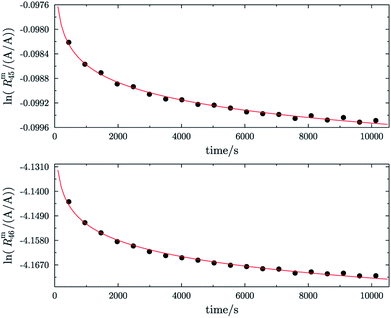
Fig. 1 shows one of the first measurements of blend b1 plotted as the natural logarithms of the ratios Rm45 (top) and Rm46 (bottom) against the time during the measurement. Time zero t0 is the time when the valve separating the bellows from the inlet system opens and the gas starts to effuse into the ionization chamber. In the case of both ratios, it can be seen that the logarithm of the ratios changes in a non-linear way. It has been shown that, in the case of a true molecular gas flow into the ionization chamber, the logarithm of the two ratios Rm45 and Rm46 should linearly increase over time during the measurement.35,37–40,46,51 This is due to the kinetic gas theory, which explains this with the faster effusion of the lighter CO2 species of mass 44. Therefore, the gas remaining in the gas reservoir becomes enriched in the heavier species, so that the measured ratios also increase. In such a case, a linear regression curve can be fitted to the data, and by extrapolation to time t0, the best guess of the measured ratio can be obtained. Before time t0, the gas can be assumed to be well mixed and it can be assumed that no mass-dependent fractionation has occurred so far. A molecular gas flow should actually not be the case for the MAT 253 with its viscous gas flow inlet system and, therefore, no mass depended fractionation should occur. However, it is known that, on the ionization source side, the gas flow necessarily becomes partly molecular and, therefore, a mass-dependent fractionation occurs.52–54 We thus expected to see a linear trend, but not as perfectly linear as with a true molecular leak since the gas flow into the ionization chamber must be assumed to be a hybrid between a viscous and a molecular flow. The deviation from the linear behaviour can also stem from a non-statistical distribution of the carbon and oxygen isotopes. If the gas is not in isotopic equilibrium (meaning a statistical isotope distribution), isotope exchange (see for example eqn (14)) reactions additionally change the measured ratio over time and, in the end, lead to non-linear behaviour. These kinds of exchange reactions are accelerated by hot surfaces like the filament of the ion source and its surroundings.35,37–40,46,51| | | 16O12C16O + 18O13C18O ⇌ 18O12C16O + 16O13C18O | (14) |
 |
| | Fig. 1 Plot of ln(Rm45) against time (top) and ln(Rm46) against time (bottom) in case of blend b1. The black dots are the measured ratios, the red lines are fits using the generic equation ln(Rmx) = a1 × ln(t) + a0. Both graphs show that the ln of both ratios does not linearly increase over time. | |
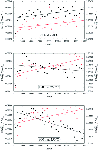
In order to obtain the isotope equilibrium, blend b1 was heated. First, moderate temperatures were used to equilibrate the parent gases and the blends, since it was unclear whether the custom-made gas spheres or the valves could resist higher temperatures. The heating temperature was set to 250 °C. After heating the blend for 72 h and letting the sphere cool down to room temperature, the isotopologue ratios were measured again. In Fig. 2, ln(Rm45) and ln(Rm46) versus time are plotted after heating blend b1 for 72 h (top subfigure), black circles and red triangles, respectively. The left y-axis is for ln(Rm45) and the right y-axis is for ln(Rm46). The red and the black lines are the corresponding linear regression fits. An increasing trend could be witnessed for both ratios, but as the deviation to a straight linear trend was quite big, the heating was continued, since we assumed that the isotopic equilibrium had not been reached. After heating the blend for in total 180 h (Fig. 2 centre), none of the two ratios showed a linear trend. ln(Rm46) hardly increased and ln(Rm45) first increased and then, after roughly 2000 s, even decreased. Since even heating for 600 h (Fig. 2 bottom) did not lead to the desired effect, the heating temperature was increased to roughly 1800 °C using a Bunsen burner. After heating blend b1 for 20 min and letting the sphere cool down to room temperature again, the measurement was repeated. The results of this measurement are shown in Fig. 3a. Again, the logarithm of the two ratios is plotted against the time. The change of ln(Rm45) over time already looks quite linear and, when compared to the first measurements without heating, it has totally changed. The change of ln(Rm46) over time, on the other hand, does not look that close to linear, but also here an improvement could be recognized. Therefore, the blend was heated longer. Fig. 3b and c show ln(Rm45) and ln(Rm46) after heating blend b1 for 84 min (1.4 h) and 270 min (4.5 h), respectively. These two figures show that, by further heating, the trend can be improved slightly to be more linear. There is still a discrepancy from the theoretically predicted linear trend. This could be explained by the fact that a linear trend is only the case when a true molecular gas flow is achieved, and also the isotopic distribution is statistical. Nevertheless, in both cases extrapolation yields values which are quite close to the theoretical values when a statistical distribution is assumed. The extrapolated values and the theoretical values are summarized in Table 9. In the first row, the two theoretical ratios are listed. In the following three rows, we see the values obtained by extrapolation to time zero, after heating the blend for 20 min (Fig. 3a), 1.4 h (Fig. 3b) and 4.5 h (Fig. 3c). In the ESI,† a script written in Isodat Scrip Language (ISL) is presented, which allows us to determine time t0. Also, a function written in Visual Basics for Applications (VBA) is added, which can be used for the extrapolation of intensity ratios at time zero as well as for the calculation of the associated uncertainties. All the ratios obtained by extrapolation are quite close to the theoretical values. A possible explanation for the deviation from the theoretical values is that no mass bias correction could be applied. The fact that the three extrapolated ratios do not fully agree with each other may be caused by the fact that mass bias changes from day to day. It is also noticeable that the extrapolated values Rm45,0 are systematically higher than Req45 (roughly 0.50%) and extrapolated values Rm46,0 are systematically lower than Req46 (roughly −0.84%).
 |
| | Fig. 2 Heating history of blend b1. Top: ln(Rm45) (black dots) and ln(Rm46) (red triangles) against time after heating at 250 °C for 72 h. Centre: ln(Rm45) and ln(Rm46) against time after heating at 250 °C for 180 h. Bottom: ln(Rm45) and ln(Rm46) against time after heating at 250 °C for 600 h. Mind the different scales. | |
 |
| | Fig. 3 ln(Rm45) and ln(Rm46) against time, after heating b1 for different amounts of time. | |
Table 9 Comparison of the theoretical ratios R45 and R46 of blend b1 and values obtained by extrapolation to time zero. Before each measurement, the blend was heated for different amounts of time (20 min, 84 min and 270 min) at ϑ ≈ 1800 °C. To calculate the theoretical values, a perfect statistical distribution of the isotopes was assumed. Stated uncertainties are expanded with k = 2
| Theoretical |
R
45 (mol mol−1) |
R
46 (mol mol−1) |
|
|
0.9094(29) |
0.0193(15) |
| Time (min) |
R
m45,0 (A/A) |
R
m46,0 (A/A) |
| 20 |
0.914081(15) |
0.0191447(26) |
| 84 |
0.913995(16) |
0.0191394(23) |
| 270 |
0.913850(18) |
0.0191292(37) |
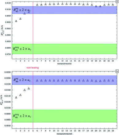
At this point, it should be mentioned that Valkiers et al.37 have developed a mathematical tool (the so-called ‘isotope equilibrium surface’) to assess the progress of the isotope equilibrium. For this tool, it is necessary to measure at least three ion intensity ratios (Valkiers et al. measured Rm45 to Rm47), otherwise not enough information about the isotopic composition is given, and the system of equations describing it cannot be solved. Since the mass spectrometer used in this study is not capable of measuring more than three ion intensities simultaneously, this handy tool could not be used. Nevertheless, it can be noted that heating does improve the repeatability as shown in Fig. 4. In this figure, Rm45,0 and Rm46,0 (both obtained by linear extrapolation to time zero) are shown for different measurements; between each measurement, blend b1 has been heated. The green areas represent the theoretical values of Rneq45 ± 2 × uc and Rneq46 ± 2 × uc, where no statistical distribution is assumed. The blue areas represent Req45 ± 2 × uc and Req46 ± 2 × uc, but this time a statistical isotope distribution is assumed. The red line indicates when heating the blend has started. The first four measurements were performed without prior heating. These extrapolated values do not agree with the theoretical values Req45 and Req46, respectively. In both cases, heating decreases the difference between the extrapolated value and the equilibrium value, indicating that the isotope distribution has been shifted towards a statistical distribution. But there is still a huge scattering between the extrapolated values after heating the gas. In the case of Rm45,0, the relative standard deviation s45,rel is roughly 0.057%, and in the case of Rm46,0, s46,rel is roughly 0.052%. The scattering before the heating is much higher; s45,rel is roughly 0.11% and s46,rel is roughly 3.4%. The increase of the two ratios from measurements 1 to 4 indicates that the equilibrating also occurs slowly without heating. The scattering of the extrapolated values after the heating can be explained by the fact that these ratios have not been corrected for any mass bias. Also, the isotope equilibrium may not be reached entirely and another possible explanation could be contamination from previous measurements of gases with significantly different isotopic composition. In the case of Rm45, heating leads to an increase of the extrapolated value, so that, after heating, the values are out of the Req45 ± 2 × uc range. In the case of Rm46, heating also leads to an increase of the measured values, but in this case, they are all in the Req46 ± 2 × uc range. It must, however, be borne in mind that the relative uncertainty associated with Req46 is about twenty times as high as the relative uncertainty associated with Req45. Nevertheless, this shows that heating does decrease the discrepancy between the measured and the theoretical values of equilibrated gas.
 |
| | Fig. 4 Graph (a) shows Rm45,0 (obtained by extrapolation to time t0) of b1. Measurements 1 to 4 were done without previous heating. Starting from measurement 6, the blend was heated for different time intervals. Until measurement 20 the heating temperature was limited to 250 °C and afterwards increased to 1800 °C. The blue area represents the theoretical value of (Req45 ± 2 × uc) assuming a perfect statistical distribution of the isotopes. The green area indicates the theoretical value of Rneq45 without statistical distribution. Graph (b) is analogous to (a) but for Rm46,0. All error bars represent the expanded uncertainty with k = 2. | |
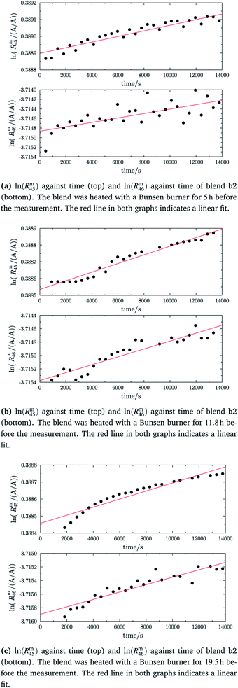
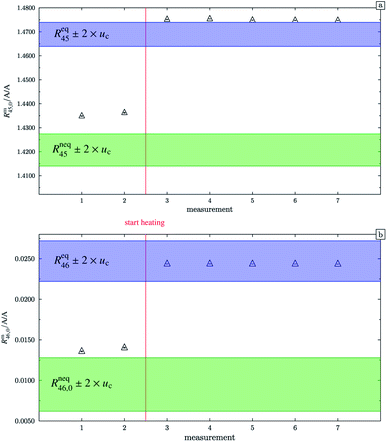
In the case of blend b2 (also prepared from A and B), similar behaviour could be witnessed. Fig. 5a–c show the logarithm of the two measured ratios plotted against time. Before the measurement, the blend was heated for 5 h, 11.8 h and 19.5 h, respectively. The values extrapolated from these measurements are compared with the theoretical values in Table 10. The comparison shows that the difference to the theoretical values is more or less the same for the three different heating times. The extrapolated values of R45 are roughly 0.41% on average higher, and the extrapolated values of R46 are roughly 1.3% on average lower than the theoretical values. This is quite similar to the situation found for blend b1. The difference for each value is of course a little different since mass bias varies from day to day. This fact, however, shows certain systematics. Since the deviation is about the same, this demonstrates that further heating does not seem to be beneficial. The deviation from the linear trend is clearly visible in all plots. The difference from the predicted behaviour can again be explained by the lack of a true molecular flow, with the possible contaminations or, despite the excessive heating, with an isotope distribution that is not truly statistical. Also drifts in the mass spectrometer, which are caused by electronic instabilities (e.g. amplifier drift, background level drift), could be possible reasons for the deviation from the linear trend. Like b1, the extrapolated values of b2 increase after heating the blend, and the difference between them and the theoretical Reqy (y ∈ {45,46}) values decreases, see Fig. 6. It is quite remarkable that after heating b2, the extrapolated values of Rm45,0 are also slightly too high and not in the Req45 ± 2 × uc range, whereas the Rm46,0 values are in the Req46 ± 2 × uc range.
 |
| | Fig. 5 ln(Rm45) and ln(Rm46) against time, after heating blend b2 for different amounts of time. | |
Table 10 Comparison of the theoretical ratios R45 and R46 of blend b2 and ratios obtained by extrapolation to time zero. Before the measurements, b2 was heated (5 h, 11.8 h and 19.5 h). For the theoretical values, a perfect statistical distribution of the isotopes was assumed
| Theoretical |
R
45 (mol mol−1) |
R
46 (mol mol−1) |
|
|
1.4689(50) |
0.0247(25) |
| Time (h) |
R
m45,0 (A/A) |
R
m46,0 (A/A) |
| 5 |
1.475354(27) |
0.0243587(32) |
| 11.8 |
1.474819(25) |
0.0243463(18) |
| 19.5 |
1.474704(39) |
0.0243337(18) |
 |
| | Fig. 6 Graph (a) shows Rm45,0 (obtained by extrapolation to time t0) of blend b2. Measurements 1 and 2 were done without previous heating. Starting from measurement 3, the blend was heated for different time intervals. The blue area represents the theoretical value of (Req45 ± 2 × uc) assuming a perfect statistical distribution of the isotopes. The green area indicates the theoretical value of Rneq45 without statistical distribution. Graph (b) is analogous to graph (a) but for Rm46,0. All error bars represent the expanded uncertainty with k = 2. | |
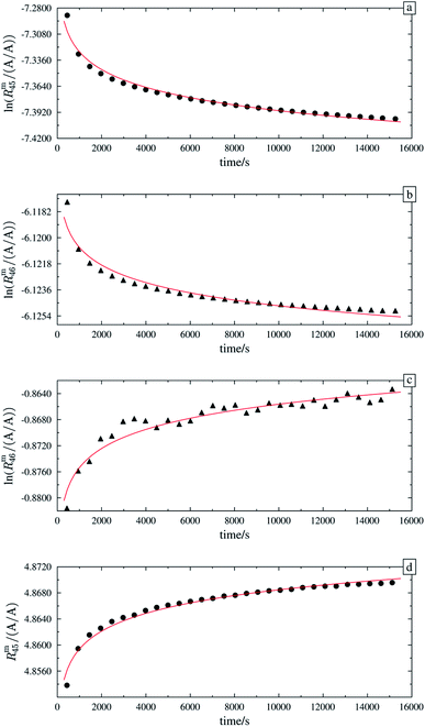
In addition, before they were equilibrated, the parent gases of b1 and b2 (A and B) showed trends which differ from the predicted linear trend, see Fig. 7. The two plots on the left show ln(Rm45) and ln(Rm46) against time of A and the corresponding fit function. The two plots on the right show ln(Rm45) and ln(Rm46) against time of B and the corresponding fit function. In both cases, the logarithm of the measured ion intensities changes in a way which can best be described by a function of the form Ry(t) = a1 × ln![[thin space (1/6-em)]](https://www.rsc.org/images/entities/char_2009.gif) t + a0. Extrapolation to t = 0 is, in such cases, not possible as ln(0) is not defined and this kind of function will not converge to a fixed value. It is also noticeable that the 12C enriched material shows a decreasing trend for both ratios, like blend b1 before heating it, and the 13C enriched material shows an increasing trend over time. It is actually not easy to tell why different trends were observed, but the deviation from the linear trend shows that the parent materials are also not equilibrated. Therefore, these two gases were heated too.
t + a0. Extrapolation to t = 0 is, in such cases, not possible as ln(0) is not defined and this kind of function will not converge to a fixed value. It is also noticeable that the 12C enriched material shows a decreasing trend for both ratios, like blend b1 before heating it, and the 13C enriched material shows an increasing trend over time. It is actually not easy to tell why different trends were observed, but the deviation from the linear trend shows that the parent materials are also not equilibrated. Therefore, these two gases were heated too.
 |
| | Fig. 7 ln(Rm45) against time and ln(Rm46) against time of the 12C enriched material A (graphs (a) and (b)). ln(Rm45) and ln(Rm46) against time of the 13C enriched material B (graphs (c) and (d)). The red lines in all four plots are fitted logarithmic curves. | |
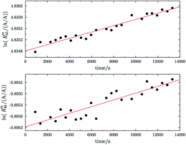
Fig. 8 shows the logarithms of Rm45 and Rm46 of B (13C enriched material) against time, after being heated for in total 13 h. Extrapolation to time t0 yielded Rm45,0 = 125.801(18) A/A and Rm46,0 = 0.480 794(16) A/A. These are quite close to the theoretical values, which are Rtheo45 = 142(24) mol mol−1 and Rtheo46 = 0.61(35) mol mol−1, respectively. The uncertainties associated with the theoretical ratios are that high as the uncertainties associated with the amount-of-substance fractions of the parent materials needed to be estimated, see Table 4. There is still a difference between the extrapolated values and the theoretical ones, which is probably caused by an insufficient statistical isotopic distribution, contamination from previous measurements of other gases and also the fact that extrapolated values have not been corrected for any mass bias, since the K-factors are still unknown. The fact that both ratios are roughly 20% lower than the theoretical values, indicates that – despite intense heating – the isotopic equilibrium has not yet been reached.55 The uncertainties associated with Rtheo45 and Rtheo43 are quite high, since we needed to estimate the uncertainties associated with amount-of-substance fractions of the isotopes, see Table 4.
 |
| | Fig. 8 Logarithms of Rm45 (top) and Rm46 (bottom) against time during the measurement of parent material B (13C enriched material). The gas was heated prior to the measurement for 13 h using a Bunsen burner (ϑ ≈ 1800 °C). | |
As already mentioned, the 12C enriched material (A) also showed non-linear behaviour in the first measurements, see Fig. 7 (left two plots). Therefore, it has also been heated. In Fig. 9a, again the logarithms of Rm45 and Rm46 against time are plotted. Both ratios show a nearly perfect linear trend, but unlike the prediction of the kinetic gas theory and in the cases of B, b1 and b2, the ratios decrease over time. A decreasing trend would mean that the remaining gas in the reservoir (bellows) becomes lighter instead of heavier due to the faster effusion of the lighter species. The decreasing linear trend most likely indicates that even after 25 h of heating the gas with a Bunsen burner, the isotopic equilibrium has not been reached completely. The extrapolated values of Rm45 and Rm46 also indicate that. The extrapolation yields Rm45,0 = 0.00061533(14) A/A and Rm46,0 = 0.002187739(67) A/A, and the theoretical values are Rtheo45 = 0.00080(16) mol mol−1 and Rtheo46 = 0.00341(23) mol mol−1, respectively. Both ratios are lower than the theoretical values, roughly 30% in the case of Rm45,0 and roughly 55% in the case of Rm46,0. This again indicates that the equilibrium has not been reached so far. One possible explanation for the different behaviour of A compared to the blends is that the gas-to-surface ratio in the lecture bottles is much smaller than in our custom-made spheres. For instance, the gas pressure in our spheres is roughly 2 bar and the volume of the spheres is approximately 800 mL; the gas pressure in the lecture bottle containing A is roughly 10 bar, and the volume is less than 500 mL. Since the isotope exchange reactions mainly occur during adsorption and desorption, a higher number of adsorption sites (larger surface) should faster lead to an equilibration. In order to improve the gas-to-surface ratio, an aliquot (roughly 1 bar) of this gas was filled in one of the gas spheres. This aliquot was subsequently heated for another 48 h with a Bunsen burner (ϑ ≈ 1800 °C). In Fig. 9b, it can be seen that – despite increasing the surface and heating the gas for a longer period – the logarithm of Rm45 and Rm46 still decreases linearly instead of increasing linearly. Although the trend is still wrong, we fitted linear functions to the data and obtained Rm45,0 and Rm46,0 and compared them to the theoretical values, see Table 11. In both cases, the difference to the theoretical values is still huge, roughly 33% in the case of Rm45,0 and roughly 55% in the case of Rm46,0. These are more or less the same differences as before filling the gas into one of the spheres. This shows that only increasing the surface does not lead to the expected linear increasing trend. Nevertheless, fractionation effects originating from the filling could have changed the isotopic composition of the gas in the sphere and since these effects can hardly be avoided must also be considered for the difference of the values. It is known that the isotopic equilibrium is reached faster when a catalyst like a platinum powder or mesh is additionally used.46,56 At the beginning of this study, we avoided using a catalyst since the huge surface of a catalyst does not only enhance the exchange reactions but is also a potential source of contamination like water or carbon dioxide from ambient air. However, as heating alone was not successful in this case, we needed to reconsider. Another aliquot of A (1.8 bar) was filled in a sphere. Previous to the filling, a platinum band (m ≈ 1 g) was placed into the sphere. Since such a catalyst is a potential source of any kind of contamination, the gas sphere (containing the catalyst) was heated (ϑ ≈ 450 °C) and evacuated for 9 h, till the pressure dropped down below 1 × 10⁻⁴ Pa. In the following step, the sphere was heated again using a Bunsen burner for 39.5 h, and afterwards the measurement was repeated. In Fig. 9c, the logarithms of Rm45 (top) and Rm46 (bottom) are plotted against time during the measurement. Additionally for orientation, a linear fit is plotted (in the case of Rm45 only the first 6000 s were considered). It is quite obvious that both ratios do not change over time as expected by theory. In the first 6000 s, ln(Rm45) behaves quite linearly, if the first two data points are neglected. After this time, the trend changes to be slowly decreasing. The logarithm of Rm46, on the other hand, shows a decreasing trend right from the start of the measurement, which can hardly be described with a linear function. Nevertheless, in Table 11, Rm45,0 and Rm46,0, both obtained via linear extrapolation to t0, are compared to the theoretical values. Moreover, as in the previous experiments, where we heated the gas in the lecture bottle and in one of our spheres, the difference to the theoretical values is quite huge (compared to what could be obtained in the cases of b1 and b2). With roughly 34% (Rm45,0) and 52% (Rm46,0), nearly the same difference to the theoretical values was obtained again. For b1 and b2, simple heating seems to be sufficient. In the case of the 12C enriched material, none of our approaches (heating, heating and increasing the gas-to-surface ratio, using a catalyst) led to the desired behaviour. This gives rise to the question of why 12C enriched gas behaves differently. We assume that in the case of a highly 12C enriched (and therefore very light) gas, other effects like the viscosity η, which controls the viscous gas flow,53 are enhanced. The viscosity, on the other hand, depends on the composition of the gas in an unforeseeable way.53 Therefore, it might be worth testing a true molecular leak. The reasons for the different behaviour of A need to be investigated further.
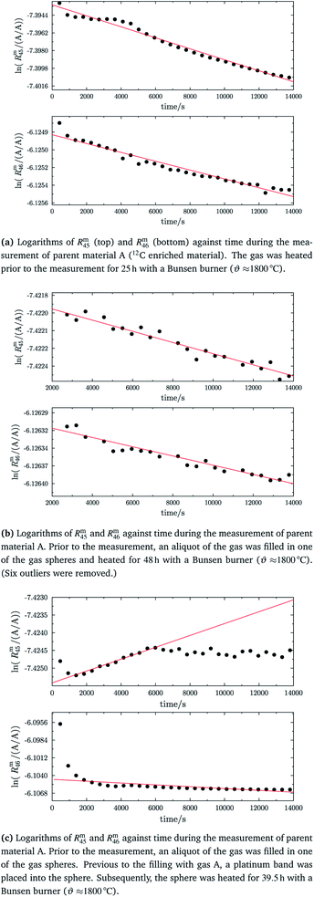 |
| | Fig. 9 ln(Rm45) and ln(Rm46) against time, after heating parent material A for different amounts of time. | |
Table 11 Comparison of the theoretical ratios R45 and R46 and ratios obtained by extrapolation to the time zero obtained using parent material A. Previous to the measurements, material A was heated (25 h, 48 h in sphere and 39.5 h in sphere in the presence of a Pt catalyst). For the theoretical values, a perfect statistical distribution of the isotopes was assumed. All stated uncertainties are expanded with k = 2
| Theo. |
R
45 (mol mol−1) |
R
46 (mol mol−1) |
|
|
0.00080(16) |
0.00341(23) |
| Time (h) |
R
m45,0 (A/A) |
R
m46,0 (A/A) |
Comment |
| 25 |
0.00061533(14) |
0.002187739(67) |
Lecture bottle |
| 48 |
0.000598048(23) |
0.002184654(18) |
Sphere |
| 39.5 |
0.000596193(84) |
0.0022326(10) |
Sphere + Pt |
Thus, we also filled an aliquot (roughly 1 bar) of a CO2 with natural isotopic composition (δVPDB13C = (−17.526 ± 0.016)‰ and δCO218O = (−10.118 ± 0.0119)‰, with k = 1 in both cases) in one of our spheres and heated it (30 min at 1800 °C). Afterwards, we measured it just like the parent materials or blends. Also in this case, we could observe that the logarithm of the two measured ratios decreased linearly over time, the plot can be found in the ESI.† Also the natural, and therefore also very light, CO2 shows this behaviour, this could be a hint that in the case of light gases the flow has a bigger influence on the measured ratios over time.
Nevertheless, it is worth trying to use the data set of blend b1 and the two parent materials to investigate whether our approach works. The procedure is described in the following section.
5.2 Simulation
The new approach shown above of calculating the wanted K-factors needs to be tested. But first, an obstacle had to be overcome. As mentioned already, the mass spectrometer used in this study is not capable of measuring four cardinal masses of CO2 simultaneously. Therefore, we needed to calculate the measured ratio Rm47 from Rm45 and Rm46. This procedure is shown in the ESI.†
With these simulated values of Rm47,y (y ∈ {A, B, AB}), we were able to conduct our simulation testing of the approach described above. For this simulation, we used the data set shown in Table 12, whereas the values of R45 and R46 were obtained by extrapolation (measurements of A, B, and b1) and the values of R47 were simulated as mentioned above (we therefore marked them with an ‘*’). The atomic masses of the two stable carbon and three stable oxygen isotopes used in this simulation are not listed here. They were taken from Wang.44 The masses of A and B stem from the preparation of b1. These values were entered in the Mathematica® notebook. The K-factors and absolute isotope ratios obtained are listed in Table 13. The results clearly show that no reasonable K-factors can be calculated with the data used. K45 seems to be reasonable, since it is close to one, but the two other K-factors are much too high. Possible reasons for these strange results could be that at least parent material A is not in isotope equilibrium and/or, for the calculation of R47, we used K and λ as recommended by Brand.57 Actually, setting the value of λ to 0.528 is only strictly appropriate for natural CO2, where the oxygen mainly stems from the global water pool, which has a λ of 0.528.58–60 It might be doubtful that this value of λ is also valid for the gases in this study, but as there is no alternative, we decided to use it anyway. The number of unknowns could otherwise not be reduced so that the equations could be solved. As no useful values were obtained, the calculation of the uncertainties was omitted. This simulation neither proves nor disproves our approach, but clearly shows its limitations. The gases really need to be in isotopic equilibrium and, also, at least three ion intensity ratios must be measured.
Table 12 Input of the first simulation with real numbers obtained from measurements of the two parent materials A and B and the binary blend b1. Material A was heated for 25 h, material B for 13 h, and blend b1 for 4.5 h, all at ϑ ≈ 1800 °C. The values of Rm45 and Rm46 were obtained from extrapolation;  was calculated as shown above
|
|
A |
B |
b1 |
|
R
m45 (A/A) |
0.00061533 |
125.8005162 |
0.913849839 |
|
R
m46 (A/A) |
0.002187739 |
0.407936972 |
0.019129236 |

|
0.000000735 |
6.058849574 |
0.016065393 |
|
m
X (g) |
0.813116 |
0.765261 |
|
Table 13 Results obtained from the input shown in Table 12
|
K
45 (mol mol−1) (A A−1)−1 |
0.991111 |
|
K
46 (mol mol−1) (A A−1)−1 |
29.4996 |
|
K
47 (mol mol−1) (A A−1)−1 |
29.8689 |
| Absolute ratios |
A |
B |
|
R
13,y (mol mol−1) |
0.000070479 |
124.597 |
|
R
17,y (mol mol−1) |
0.000269691 |
0.0424648 |
|
R
18,y (mol mol−1) |
0.0322686 |
0.725074 |
Table 14 Initial values of the isotope ratios R13,y, R17,y and R18,y (y is A′, B′ or AB′). These values need to be calculated
| Initial K-factors (mol mol−1) (A A−1)−1 |
|
K
45
|
0.9530 |
|
K
46
|
0.8301 |
|
K
47
|
0.7943 |
|
|
A′ |
B′ |
AB′ |
|
R
13,y (A/A) |
0.0108157 |
79.6451613 |
0.981306781 |
|
R
17,y (A/A) |
0.0003809 |
0.0099800 |
0.005092367 |
|
R
18,y (A/A) |
0.0020550 |
0.0136138 |
0.007728291 |
In order to test our approach we tried it with a made-up data set, which allowed us to avoid the issues described above. Please note that the nomenclature was changed in order to separate the made-up simulation data clearly from the real life data set, A → A′. The amount-of-substance fractions (x(13C) to x(18O)) of material A′ were chosen to be the IUPAC values,61 so that it can be regarded as a ‘natural’ material, which could be used as a new reference material. From the absolute isotope ratios, we calculated the isotopologue ratios (R45, R46 and R47), and finally the measured ratios using eqn (1). The whole data set was entered into our Mathematica® notebook, and the calculation was repeated. The input is listed in the ESI, Table S1.† For this simulation, also the uncertainties associated with the isotope ratios and the K-factors, respectively, were calculated. This was done via a Monte Carlo simulation, with 105 trials. The relative uncertainties stem from our real measurements and, therefore, should be adequate for this performance test. The results are shown in Table 15. The obtained PDFs and histograms can be seen in the ESI.† Please note, the absolute isotope ratios of blend AB′ are not a direct result of our approach and, therefore, not listed here, but they can easily be calculated using the K-factors obtained. It is commonly agreed that for a robust δ scale, the absolute ratio R13C/12C of the zero point (VPDB) must be known with a relative uncertainty of 0.01‰ or lower.23 This means that also the relative uncertainty associated with the absolute isotope ratio of material A′ must be less than 0.01‰.
Table 15 Results obtained from the made-up input shown in Table 14. All uncertainties are standard uncertainties (k = 1)
|
K-Factors |
|
u
rel (%) |
|
K
45 (mol mol−1) (A A−1)−1 |
0.95298(34) |
0.036 |
|
K
46 (mol mol−1) (A A−1)−1 |
0.830(11) |
1.34 |
|
K
47 (mol mol−1) (A A−1)−1 |
0.794(12) |
1.50 |
| Absolute ratios |
A′ |
|
|
R
13 (mol mol−1) |
0.010815(38) |
0.35 |
|
R
17 (mol mol−1) |
0.000381(18) |
4.74 |
|
R
18 (mol mol−1) |
0.002055(28) |
1.35 |
| Absolute ratios |
B′ |
|
|
R
13 (mol mol−1) |
79.645(28) |
0.036 |
|
R
17 (mol mol−1) |
0.00998(13) |
1.31 |
|
R
18 (mol mol−1) |
0.01362(20) |
1.49 |
In Table 15, also the relative uncertainties are given. For the assessment of the performance in terms of achievable uncertainties, only material A′ is considered, since it could be a reference material candidate. The uncertainties associated with the absolute isotope ratios of material A′ are quite high. urel(R13C/12C) is more than two orders of magnitude higher than the upper limit defined by the requirement stated earlier. In order to clarify which quantity contributes the most to the uncertainties of the absolute ratios of material A′, the budgets of u(R13,A′), u(R17,A′) and u(R18,A′) were also calculated. This was done by all Monte Carlo simulations.62,63 The three budgets are given in Table 16, where only the uncertainty contribution ui of every input xi and the relative contribution (rel. ui), which is ui2/uc2, are listed. The three budgets reveal that the contributions of the ratios Rm47,A′, Rm47,B′ and Rm47,AB′ especially dominate the uncertainty budgets of the three absolute ratios. In all three cases, the sum of these three contributions is more than 75%. Normally, the uncertainty contribution stemming from the masses is the highest part for absolute ratios obtained by gravimetric mixtures. One possible reason for the very high contributions of the three Rm47,Y ratios is that the relative uncertainties associated with them stem from our first simulation. In this simulation, Rm47,Y needed to be derived from the corresponding Rm45,Y and Rm46,Y and therefore u(Rm45,Y) and u(Rm46,Y) contribute to u(Rm47,Y) and probably increase it artificially. The achievable u(Rm47,Y) stemming from real measurements are probably much smaller, which will reduce the combined uncertainty associated with the absolute ratios. Also, with this simulation, using a made-up data set, the performance of our approach cannot yet be finally assessed.
Table 16 Uncertainty budget of the three absolute ratios of material A′ obtained by applying our approach
|
x
i
|
R
13,A′
|
R
17,A′
|
R
18,A′
|
|
u
i
(mol mol−1) |
Rel. ui (%) |
u
i
(mol mol−1) |
Rel. ui (%) |
u
i
(mol mol−1) |
Rel. ui (%) |
|
M(13C) |
1.5 × 10⁻¹³ |
1.5 × 10⁻¹⁵ |
3.9 × 10⁻¹⁴ |
4.7 × 10⁻¹⁶ |
2.0 × 10⁻¹³ |
5.3 × 10⁻¹⁵ |
|
M(16O) |
9.9 × 10⁻¹⁵ |
6.8 × 10⁻¹⁸ |
3.9 × 10⁻¹⁴ |
4.7 × 10⁻¹⁶ |
1.3 × 10⁻¹⁴ |
2.4 × 10⁻¹⁷ |
|
M(17O) |
1.0 × 10⁻¹⁴ |
7.4 × 10⁻¹⁸ |
2.7 × 10⁻⁹ |
2.3 × 10⁻¹⁸ |
1.4 × 10⁻¹⁴ |
2.6 × 10⁻¹⁷ |
|
M(18O) |
8.6 × 10⁻¹⁵ |
5.1 × 10⁻¹⁸ |
2.3 × 10⁻¹⁵ |
1.6 × 10⁻¹⁸ |
1.2 × 10⁻¹⁴ |
1.8 × 10⁻¹⁷ |
|
m
A′
|
5.7 × 10⁻⁶ |
2.2 × 100 |
1.5 × 10⁻⁶ |
6.9 × 10⁻¹ |
7.7 × 10⁻⁶ |
7.7 × 100 |
|
m
B′
|
5.6 × 10⁻⁶ |
2.2 × 100 |
1.5 × 10⁻⁶ |
6.9 × 10⁻¹ |
7.7 × 10⁻⁶ |
7.7 × 100 |
|
R
m45,A′
|
4.2 × 10⁻⁶ |
1.2 × 100 |
2.8 × 10⁻⁶ |
2.4 × 100 |
2.6 × 10⁻⁶ |
8.6 × 10⁻¹ |
|
R
m46,A′
|
5.4 × 10⁻⁷ |
2.0 × 10⁻² |
2.7 × 10⁻⁷ |
2.3 × 10⁻² |
5.0 × 10⁻⁷ |
3.3 × 10⁻² |
|
R
m47,A′
|
9.8 × 10⁻⁶ |
6.7 × 100 |
5.0 × 10⁻⁶ |
7.5 × 100 |
4.6 × 10⁻⁶ |
2.7 × 100 |
|
R
m45,B′
|
2.3 × 10⁻⁶ |
3.8 × 10⁻¹ |
2.8 × 10⁻⁶ |
2.4 × 100 |
2.6 × 10⁻⁶ |
8.6 × 10⁻¹ |
|
R
m46,B′
|
4.7 × 10⁻⁶ |
1.5 × 100 |
2.4 × 10⁻⁶ |
21.8 × 100 |
3.9 × 10⁻⁶ |
2.0 × 100 |
|
R
m47,B′
|
2.4 × 10⁻⁵ |
4.2 × 101 |
1.2 × 10⁻⁵ |
4.1 × 101 |
2.2 × 10⁻⁵ |
6.3 × 101 |
|
R
m45,AB′
|
7.9 × 10⁻⁷ |
4.3 × 10⁻² |
4.3 × 10⁻⁷ |
5.7 × 10⁻² |
5.0 × 10⁻⁴ |
3.2 × 10⁻² |
|
R
m46,AB′
|
5.9 × 10⁻⁶ |
2.4 × 100 |
3.0 × 10⁻⁶ |
2.8 × 100 |
5.3 × 10⁻⁶ |
3.7 × 100 |
|
R
m47,AB′
|
2.5 × 10⁻⁵ |
4.2 × 101 |
1.2 × 10⁻⁵ |
4.3 × 101 |
8.7 × 10⁻⁶ |
9.9 × 100 |
6 Conclusion and outlook
In this publication, we have shown that the gravimetric mixture approach for calculating K-factors according to ref. 31 for a system consisting of several isotopologues does not work since the isotopic equilibrium is not considered in the original approach. Not considering the isotopic equilibrium leads to wrong K-factors and, in the end, to incorrectly determined isotope ratios. We presented an alternative mathematical ansatz which considers the isotopic equilibrium. Applying this approach, only two parent materials and one binary blend are necessary, and only three intensity ratios per gas must be measured. This is an immense reduction of the blends needed and ratios measured compared to the classical approach. For the calculation of the wanted K-factors, it is necessary to solve a system of non-linear equations. In the ESI† of this publication, a Mathematica® notebook is presented which allows the calculation of the K-factors, the absolute isotope ratios of the two parent materials and the uncertainties associated with them. In addition to the theoretical work, we showed the first attempts of applying our new approach by preparing binary mixtures from isotopically enriched parent materials. Two different blends from enriched parent materials were prepared.
For our approach, the parent materials and the blend must be equilibrated. In the cases of our two blends, we showed that heating them with a Bunsen burner (even without the use of a catalyst) seems to be the right way to equilibrate the gas. Unfortunately, equilibrating the 12C enriched parent material was not successful, and further investigations into the reasons are necessary. Nevertheless, with a simulation that was as real as possible, we showed that our approach in principal works, but the achieved uncertainties were not sufficient to fulfil the metrological requirements for establishing a robust and SI-traceable δ scale. It has to be stressed that some of the uncertainties used were conservative (due to measurement limitations), and therefore, it is likely that, with measurements including more than two intensity ratios, the performance of our approach will be improved.
At this point it is worth to compare the previous work of Valkiers36 and Varlam,35 both conducted at the IRMM, with ours. First, it must be mentioned that they used a completely different type of gas mass spectrometer. The Avogadro II amount comparator (a modified MAT271) at IRMM can measure four ion intensities sequentially and therefore they did not need to make any assumptions for the calculation of the K-factors. Additionally, the Avogadro II amount comparator had a molecular inlet system. The MAT253 (a true δ machine) can hardly be compared with the mass spectrometer used at IRMM. This fact could be an explanation for the issues we encountered. Also their mathematical approach is slightly different, because we solve a system of non-linear equations, where the number of unknowns equals the number of given equations. This is a good basis for analytical solutions for the K-factors, which is a further task that needs to be tackled, since this would eliminate the risk of convergence issues. The mathematical approach of Valkiers can only be solved iteratively, which can lead to convergence issues or local minima, resulting in incorrect K-factors. Furthermore, in our approach the calculation of the associated uncertainties is done via a Monte Carlo simulation, which leads to more reliable values of the best estimates and their associated uncertainties. Also, our improved buoyancy49,50 correction is completely different.
Our approach bears some advantages which justify further efforts to improve it. Firstly, our approach considers the isotope equilibrium, secondly, the number of needed binary mixtures is reduced in comparison to the classical approach, and last but not least, it is not necessary to resolve all isotopologues. Therefore, we are convinced that further investigations will pay off.
Analogous to the works of Santamaria-Fernandez,64,65 Dunn20,21 and Malinovsky,19,22 it could be beneficial to test our approach using atomic spectrometry methods, like inductively coupled plasma mass spectrometry (ICP-MS). In these studies the ion intensity ratio 13C+/12C+ were measured directly. The advantage of such an approach would be that isotope exchange reactions during the measurement should not influence the result and memory effects in the ion source are not that critical. Since 13C+/12C+ can be measured directly, the calculation of the K-factor (and its associated uncertainty) can be simplified tremendously – useful tools were published.31,42 Also no assumptions for the 17O corrections are needed. Furthermore, with the latest advances in the field of high resolution ICP-MS and 1013 Ω amplifier resistors maybe it is even possible to measure also 18O+/16O+. These advantages and the technological progress may lead to lower achievable uncertainties, making the atomic spectrometry methods also a promising option.
7 Appendix
7.1 System of non-linear equations
The nine equations of option 01 must be solved for the unknown K-factors and the absolute isotope ratios of the two parent materials. In the ESI† a Mathematica® notebook containing a solving routine, is given. Solving the analogous equations of the nine other options can in principle be done in the same way.
Equations for parent material A.
| | | 0 = K45 × Rm45,A − (2 × R17,A + R13,A) | (15a) |
| | | 0 = K46 × Rm46,A − (2 × R18,A + R17,A2 + 2 × R13,A × R17,A) | (15b) |
| | | 0 = K47 × Rm47,A − (2 × R17,A × R18,A + 2 × R13,A × R18,A + R13,A × R17,A2) | (15c) |
Equations for parent material B.
| | | 0 = K45 × Rm45,B − (2 × R17,B + R13,B) | (16a) |
| | | 0 = K46 × Rm46,B − (2 × R18,B + R17,B2 + 2 × R13,B × R17,B) | (16b) |
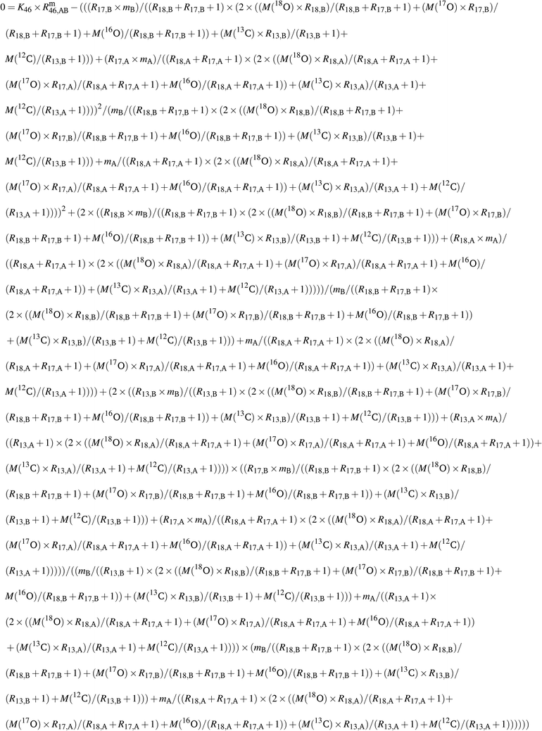
| | | 0 = K47 × Rm47,B − (2 × R17,B × R18,B + 2 × R13,B × R18,B + R13,B × R17,B2) | (16c) |
Equations for binary blend AB. Unfortunately further simplification, even using a computer algebra system, did not reduce the length of these equations, and therefore, we were forced to show them like that.
| |  | (17) |
| |  | (18) |
| |  | (19) |
Conflicts of interest
There are no conflicts to declare.
Acknowledgements
We gratefully acknowledge the support of the Braunschweig International Graduate School of Metrology (B-IGSM). The EMPIR initiative is co-funded by the European Union's Horizon 2020 Research and Innovation Programme and the EMPIR Participating States.
Notes and references
-
J. Irrgeher and T. Prohaska, in Sector Field Mass Spectrometry for Elemental and Isotopic Analysis, The Royal Society of Chemistry, 2015, pp. 107–120 Search PubMed.
- H. C. Urey, H. A. Lowenstam, S. Epstein and C. R. McKinney, Geol. Soc. Am. Bull., 1951, 62, 399 CrossRef CAS.
- I. Friedman, J. O'Neil and G. Cebula, Geostand. Geoanal. Res., 1982, 6, 11–12 CrossRef CAS.
- R. Gonfiantini, Chem. Geol., 1984, 46, 85 CrossRef.
-
G. Hut, Consultants' group meeting on stable isotope reference samples for geochemical and hydrological investigations, 1987 Search PubMed.
-
R. Gonfiantini, W. Stichler and K. Rozanski, Standards and intercomparison materials distributed by the International Atomic Energy Agency for stable isotope measurements, 1995 Search PubMed.
- T. B. Coplen, C. Kendall and J. Hopple, Nature, 1983, 302, 236–238 CrossRef CAS.
- H. Meijer, R. Neubert and G. Visser, Int. J. Mass Spectrom., 2000, 198, 45–61 CrossRef CAS.
- G. D. Flesch, A. R. Anderson and H. J. Svec, Int. J. Mass Spectrom. Ion Phys., 1973, 12, 265–272 CrossRef CAS.
- T. B. Coplen, W. A. Brand, M. Gehre, M. Gröning, H. A. J. Meijer, B. Toman and R. M. Verkouteren, Anal. Chem., 2006, 78, 2439–2441 CrossRef CAS.
-
18th WMO/IAEA Meeting on Carbon Dioxide, Other Greenhouse Gases and Related Measurement Techniques (GGMT-2015), 2015 Search PubMed.
- H. Qi, T. B. Coplen, S. J. Mroczkowski, W. A. Brand, L. Brandes, H. Geilmann and A. Schimmelmann, Rapid Commun. Mass Spectrom., 2016, 30, 859–866 CrossRef CAS.
-
Standard Atomic Weights of 14 Chemical Elements Revised, 2018, https://www.degruyter.com/view/j/ci.2018.40.issue-4/ci-2018-0409/ci-2018-0409.xml Search PubMed.
- H. Craig, Geochim. Cosmochim. Acta, 1957, 12, 133–149 CrossRef CAS.
- Q. L. Zhang, T. L. Chang and W. J. LI, Chin. Sci. Bull., 1990, 35, 290–296 CAS.
-
J. Nørgaard, H. Kipphardt, S. Valkiers and P. Taylor, Certification report EUR 19061 EN, 1999 Search PubMed.
- K. Ruße, S. Valkiers and P. Taylor, Int. J. Mass Spectrom., 2004, 235, 255–262 CrossRef.
- J. Kaiser, Geochim. Cosmochim. Acta, 2008, 72, 1312–1334 CrossRef CAS.
- D. Malinovsky, P. J. H. Dunn and H. Goenaga-Infante, J. Anal. At. Spectrom., 2013, 28, 1760 RSC.
- P. J. Dunn, M. Bilsel, A. Şimşek, A. C. Gören, M. Tunç, N. Ogrinc, M. Horvat and H. Goenaga-Infante, Rapid Commun. Mass Spectrom., 2019, 33, 1122–1136 CrossRef CAS.
- P. J. H. Dunn, D. Malinovsky and H. Goenaga-Infante, Anal. Bioanal. Chem., 2015, 407, 3169–3180 CrossRef CAS.
- D. Malinovsky, P. J. H. Dunn, G. Holcombe, S. Cowen and H. Goenaga-Infante, J. Anal. At. Spectrom., 2019, 34, 147–159 RSC.
- P. J. Brewer, J. S. Kim, S. Lee, O. A. Tarasova, J. Viallon, E. Flores, R. I. Wielgosz, T. Shimosaka, S. Assonov, C. E. Allison, A. M. H. van der Veen, B. Hall, A. M. Crotwell, G. C. Rhoderick, J. T. Hodges, J. Mohn, C. Zellweger, H. Moossen, V. Ebert and D. W. T. Griffith, Metrologia, 2019, 56, 034006 CrossRef CAS.
-
IAEA, Reference Sheet for IAEA-603, International Atomic Energy Agency technical report, 2016 Search PubMed.
- M. Wendeberg, J. Richter, M. Rothe and W. A. Brand, Atmos. Meas. Tech., 2013, 6, 817–822 CrossRef CAS.
-
Expert Group Recommendations, 16th WMO/IAEA Meeting on Carbon Dioxide, other Greenhouse Gases, and Related Measurement Techniques (GGMT-2011) (Wellington, New Zealand, 25 to 28 October 2011), ed. G. Brailsford, WMO, Geneva, 2012 Search PubMed.
- P. J. Brewer, R. J. Brown, O. A. Tarasova, B. Hall, G. C. Rhoderick and R. I. Wielgosz, Metrologia, 2018, 55, S174 CrossRef CAS.
- A. O. Nier, Phys. Rev., 1950, 77, 789–793 CrossRef CAS.
- L. Yang, S. Tong, L. Zhou, Z. Hu, Z. Mester and J. Meija, J. Anal. At. Spectrom., 2018, 1849–1861 RSC.
- G. Mana and O. Rienitz, Int. J. Mass Spectrom., 2010, 291, 55–60 CrossRef CAS.
- A. Stoll-Werian, L. Flierl, O. Rienitz, J. Noordmann, R. Kessel and A. Pramann, Spectrochim. Acta, Part B, 2019, 76–83 CrossRef CAS.
- B. Güttler, H. Bettin, R. J. C. Brown, R. S. Davis, Z. Mester, M. J. T. Milton, A. Pramann, O. Rienitz, R. D. Vocke and R. I. Wielgosz, Metrologia, 2019, 56, 044002 CrossRef.
- B. Brandt, J. Vogl, J. Noordmann, A. Kaltenbach and O. Rienitz, J. Anal. At. Spectrom., 2016, 31, 179–196 RSC.
- J. Vogl, B. Brandt, J. Noordmann, O. Rienitz and D. Malinovskiy, J. Anal. At. Spectrom., 2016, 31, 1440–1458 RSC.
- M. Varlam, S. Valkiers, M. Berglund, P. Taylor, R. Gonfiantini and P. D. Bièvre, Int. J. Mass Spectrom., 2008, 269, 78–84 CrossRef CAS.
- S. Valkiers, M. Varlam, K. Ruße, M. Berglund, P. Taylor, J. Wang, M. Milton and P. D. Bièvre, Int. J. Mass Spectrom., 2007, 264, 10–21 CrossRef CAS.
- S. Valkiers, M. Varlam, K. Ruße, M. Berglund, P. Taylor, J. Wang, M. Milton and P. D. Bièvre, Int. J. Mass Spectrom., 2007, 263, 195–203 CrossRef CAS.
- S. Valkiers, M. Varlam, M. Berglund, P. Taylor, R. Gonfiantini and P. D. Bièvre, Int. J. Mass Spectrom., 2008, 269, 71–77 CrossRef CAS.
- R. Gonfiantini, S. Valkiers, P. D. Taylor and P. De Bièvre, Int. J. Mass Spectrom. Ion Processes, 1997, 171, 231–242 CrossRef CAS.
- R. Gonfiantini, S. Valkiers, P. D. Taylor and P. D. Bièvre, Int. J. Mass Spectrom. Ion Processes, 1997, 163, 207–219 CrossRef CAS.
- R. Gonfiantini, S. Valkiers, P. D. Taylor and P. D. Bièvre, Int. J. Mass Spectrom. Ion Processes, 1997, 161, 15–26 CrossRef CAS.
- L. Flierl, A. Pramann, J. Noordmann, A. Röthke and O. Rienitz, Spectrochim. Acta, Part B, 2020, 168, 105866 CrossRef CAS.
- L. Gordon, L. Rothman, C. Hill, R. Kochanov, Y. Tan, P. Bernath, M. Birk, V. Boudon, A. Campargue, K. Chance, B. Drouin, J.-M. Flaud, R. Gamache, J. Hodges, D. Jacquemart, V. Perevalov, A. Perrin, K. Shine, M.-A. Smith, J. Tennyson, G. Toon, H. Tran, V. Tyuterev, A. Barbe, A. Császár, V. Devi, T. Furtenbacher, J. Harrison, J.-M. Hartmann, A. Jolly, T. Johnson, T. Karman, I. Kleiner, A. Kyuberis, J. Loos, O. Lyulin, S. Massie, S. Mikhailenko, N. Moazzen-Ahmadi, H. Müller, O. Naumenko, A. Nikitin, O. Polyansky, M. Rey, M. Rotger, S. Sharpe, K. Sung, E. Starikova, S. Tashkun, J. V. Auwera, G. Wagner, J. Wilzewski, P. Wcisło, S. Yu and E. Zak, J. Quant. Spectrosc. Radiat. Transfer, 2017, 203, 3–69 CrossRef.
- M. Wang, G. Audi, F. Kondev, W. Huang, S. Naimi and X. Xu, Chin. Phys. C, 2017, 41, 030003 CrossRef.
-
Commission on Isotopic Abundances and Atomic Weights, Current atomic masses, https://www.ciaaw.org/atomic-masses.htm Search PubMed.
- R. Gonfiantini, S. Valkiers, P. D. P. Taylor and P. De Bièvre, Int. J. Mass Spectrom. Ion Processes, 1997, 161, 15–26 CrossRef CAS.
-
Wolfram Research Inc., Mathematica, Version 12.0, Champaign, IL, 2019, 2019, https://www.wolfram.com/mathematica Search PubMed.
-
Joint Committee for Guides in Metrology, JCGM 100: Evaluation of Measurement Data – Guide to the Expression of Uncertainty in Measurement, JCGM technical report, 2008 Search PubMed.
- L. Flierl, O. Rienitz and A. Pramann, Anal. Bioanal. Chem., 2020, 412, 1–3 CrossRef CAS.
- L. Flierl, O. Rienitz and A. Pramann, Anal. Bioanal. Chem., 2020, 412, 3957–3959 CrossRef CAS.
- R. Gonfiantini, P. de Bièvre, S. Valkiers and P. D. P. Taylor, IEEE Trans. Instrum. Meas., 1997, 46, 566–571 CrossRef CAS.
- R. E. Honig, J. Appl. Phys., 1945, 16, 646–654 CrossRef CAS.
-
J. Roboz, Introduction to mass spectrometry; instrumentation and techniques, Interscience Publishers, 1968 Search PubMed.
-
P. J. Potts, A Handbook of Silicate Rock Analysis, Springer Netherlands, 1987 Search PubMed.
- R. Gonfiantini, P. de Bievre, S. Valkiers and P. D. P. Taylor, IEEE Trans. Instrum. Meas., 1997, 46, 566–571 CrossRef CAS.
- S. Valkiers, M. Varlam, K. Ruße, M. Berglund, P. Taylor, J. Wang, M. Milton and P. D. Bièvre, Int. J. Mass Spectrom., 2007, 263, 195–203 CrossRef CAS.
- W. A. Brand, S. S. Assonov and T. B. Coplen, Pure Appl. Chem., 2010, 82, 1719–1733 CAS.
- H. A. J. Meijer and W. J. Li, Isot. Environ. Health Stud., 1998, 34, 349–369 CrossRef CAS.
- E. Barkan and B. Luz, Rapid Commun. Mass Spectrom., 2005, 19, 3737–3742 CrossRef CAS.
- A. Landais, E. Barkan and B. Luz, Geophys. Res. Lett., 2008, 35, L02709 Search PubMed.
- J. R. de Laeter, J. K. Böhlke, P. D. Bièvre, H. Hidaka, H. S. Peiser, K. J. R. Rosman and P. D. P. Taylor, Pure Appl. Chem., 2003, 75, 683–800 CAS.
-
M. G. Cox and P. M. Harris, NPL Report DEM-ES-011, 2006, p. 175 Search PubMed.
-
BIPM, IEC, IFCC, ILAC, ISO, IUPAC, IUPAP and OIML, Supplement 1 to the ‘Guide to the expression of uncertainty in measurement’—propagation of distributions using a Monte Carlo method, JCGM 101: 2008, 2008 Search PubMed.
- R. Santamaria-Fernandez, Anal. Bioanal. Chem., 2010, 397, 973–978 CrossRef CAS.
- R. Santamaria-Fernandez, D. Carter and R. Hearn, Anal. Chem., 2008, 80, 5963–5969 CrossRef CAS.
Footnote |
| † Electronic supplementary information (ESI) available. See DOI: 10.1039/d0ja00318b |
|
| This journal is © The Royal Society of Chemistry 2020 |
 Open Access Article
 *a,
Olaf
Rienitz
 a,
Paul J.
Brewer
 b,
Harro A. J.
Meijer
 c and
Farilde M.
Steur
c


![[thin space (1/6-em)]](https://www.rsc.org/images/entities/char_2009.gif) 000. In Table 1, all isotopologues of CO2 are listed in increasing order of their molar mass. The natural abundances have been taken from the HITRAN2016 database.43 The molar masses and their associated expanded uncertainties (k = 2) were calculated using the atomic weights of the corresponding isotopes44,45 and the resolutions needed were calculated using these molar masses, whereas the resolutions needed were rounded to the nearest integer. Currently, there is no gas mass spectrometer available with such a high resolution. The second obstacle is that, due to the small natural abundance of 17O, 18O and 13C, isotopologues built from these three isotopes are quite rare, which makes detection – especially of 17O213C+ ions – rather difficult, see the abundances in Table 1. The third obstacle is that – at least at the moment – starting materials enriched particularly in one isotopologue are not available. The fourth obstacle is that the binary blends must be in isotopic equilibrium, meaning that the carbon and oxygen isotopes are statistically distributed over all the isotopologues. If the equilibrium has not been reached previous to the measurement, isotope exchange reactions will take place on the hot surfaces of the ion source, altering the measured ratios constantly and sometimes in an unpredictable way during the measurement.39–41,46 Additionally, if the gas is not in isotopical equilibrium, calculating the isotope ratios (R13C/12C, R17O/16O and R18O/16O) from the isotopologue ratios will fail. But if the equilibrium has been reached, the mathematics behind the gravimetric mixture method may not work any more.
000. In Table 1, all isotopologues of CO2 are listed in increasing order of their molar mass. The natural abundances have been taken from the HITRAN2016 database.43 The molar masses and their associated expanded uncertainties (k = 2) were calculated using the atomic weights of the corresponding isotopes44,45 and the resolutions needed were calculated using these molar masses, whereas the resolutions needed were rounded to the nearest integer. Currently, there is no gas mass spectrometer available with such a high resolution. The second obstacle is that, due to the small natural abundance of 17O, 18O and 13C, isotopologues built from these three isotopes are quite rare, which makes detection – especially of 17O213C+ ions – rather difficult, see the abundances in Table 1. The third obstacle is that – at least at the moment – starting materials enriched particularly in one isotopologue are not available. The fourth obstacle is that the binary blends must be in isotopic equilibrium, meaning that the carbon and oxygen isotopes are statistically distributed over all the isotopologues. If the equilibrium has not been reached previous to the measurement, isotope exchange reactions will take place on the hot surfaces of the ion source, altering the measured ratios constantly and sometimes in an unpredictable way during the measurement.39–41,46 Additionally, if the gas is not in isotopical equilibrium, calculating the isotope ratios (R13C/12C, R17O/16O and R18O/16O) from the isotopologue ratios will fail. But if the equilibrium has been reached, the mathematics behind the gravimetric mixture method may not work any more.
![[thin space (1/6-em)]](https://www.rsc.org/images/entities/char_2009.gif) 179
179![[thin space (1/6-em)]](https://www.rsc.org/images/entities/char_2009.gif) 824
824![[thin space (1/6-em)]](https://www.rsc.org/images/entities/char_2009.gif) 342
342![[thin space (1/6-em)]](https://www.rsc.org/images/entities/char_2009.gif) 502
502![[thin space (1/6-em)]](https://www.rsc.org/images/entities/char_2009.gif) 126
126![[thin space (1/6-em)]](https://www.rsc.org/images/entities/char_2009.gif) 426
426


 is the scale reading of the target sphere s at time zero (sphere is evacuated),
  is the scale reading of the target sphere at t1 (only containing the first parent gas), and
  is the scale reading of target sphere s at t2 (containing both parent gases). The scale readings of the reference sphere r (
 ,
,  and
and  ) are defined analogously, but during all these procedures, r stays evacuated. ρcal is the density of the calibration weight used for calibrating the balance. This weighing procedure and the mathematics developed allow us to determine the buoyancy-corrected masses of the two parent materials without knowing the density of a closed gas vessel (no matter whether it contains gas or is evacuated). For the uncertainty calculation of the two gas masses eqn (13a) and (13b) are the model equations and, additionally, the correlation between all balance readings recorded at the same time must be considered. The correlated quantities are summarized in Table 6. The correlation coefficients can be calculated using the usual formulas.48 Before each weighing cycle, the two spheres were cleaned with ethanol to remove fingerprints, dust and other residues. After cleaning, the spheres were placed near to the balance to equilibrate them to room temperature. This took roughly 24 h. To record the ambient conditions, an OPUS 20 THIP (Lufft, Fellbach, Germany) was used. Prior to each weighing, the corresponding sphere standing on a grounded plate was sprayed with a nitrogen ring ionizer/blow-out gun to remove electrostatic charges. Moreover, the influence of electrostatic charges was reduced by using a mechanical balance (H315, Mettler, Columbus, United States of America), which is conformity checked annually. The standard uncertainty, 0.0005 g, of the H315 can be estimated from the upper tolerance levels of repeatability and linearity. To place the spheres on the pan a polytetrafluoroethylene ring (inner diameter 40 mm, outer diameter 60 mm, height 5 mm) doped with carbon was used. The doping makes the ring conductible, reducing electrostatic effects.

![[thin space (1/6-em)]](https://www.rsc.org/images/entities/char_2009.gif) t + a0. Extrapolation to t = 0 is, in such cases, not possible as ln(0) is not defined and this kind of function will not converge to a fixed value. It is also noticeable that the 12C enriched material shows a decreasing trend for both ratios, like blend b1 before heating it, and the 13C enriched material shows an increasing trend over time. It is actually not easy to tell why different trends were observed, but the deviation from the linear trend shows that the parent materials are also not equilibrated. Therefore, these two gases were heated too.
t + a0. Extrapolation to t = 0 is, in such cases, not possible as ln(0) is not defined and this kind of function will not converge to a fixed value. It is also noticeable that the 12C enriched material shows a decreasing trend for both ratios, like blend b1 before heating it, and the 13C enriched material shows an increasing trend over time. It is actually not easy to tell why different trends were observed, but the deviation from the linear trend shows that the parent materials are also not equilibrated. Therefore, these two gases were heated too.
 was calculated as shown above

