 Open Access Article
 This Open Access Article is licensed under a Creative Commons Attribution-Non Commercial 3.0 Unported Licence
Spiers Memorial Lecture: Astrochemistry at high resolution
Cecilia
Ceccarelli

Univ. Grenoble Alpes, CNRS, IPAG, 38000 Grenoble, France. E-mail: Cecilia.Ceccarelli@univ-grenoble-alpes.fr
First published on 1st June 2023
Abstract
Astrochemistry is the science that studies the chemistry in the Universe, namely the combination of two fields: astronomy and chemistry. It started about fifty years ago and it has progressed in leaps and bounds, often triggered by the advent of new telescopes. From the collection of new interstellar molecule detections, astrochemistry has evolved more and more in the quest to understand how they are formed and thrive in the harsh conditions of the interstellar medium. Collaboration between astronomers and chemists has never been more necessary than today, when new powerful astronomical facilities provide us with ever sharper images of the regions where interstellar molecules are present. This review focuses on the special case of interstellar complex organic molecules (iCOMs), one the most debated astrochemical fields and where the astronomers–chemists collaboration and synergy is indispensable. The review will go through the various phases of the formation of planetary system similar to the solar system, providing the most recent observational picture at each step. The current scenarios of the iCOMs formation will be laid down and the critical chemical processes and quantities involved in each of them will be discussed. The major goal of this review is not only to present the progress but, more importantly, to highlight the many areas of uncertainty. A few specific cases will be discussed to give practical examples of why the huge challenge that represents the formation of iCOMs can only be won if chemists and astronomers work together.
1 Introduction
Why do we need a Faraday Discussion on astrochemistry at high resolution? The images reported in Fig. 1 say more than a thousand words: high resolution observations at different wavelengths obtained in the last decade have added so many details that astrochemistry now faces new challenges, adding to the old ones, to explain them. The figure shows only one of the numerous examples that could have been given. It shows the famous solar-type protostar NGC1333 IRAS4, a protobinary system composed of two objects, A1 and A2, separated by about 1′′.8 in the sky, equivalent to about 550 au. The figure shows methanol emission maps obtained with three different interferometers: SMA in the submillimeter (submm),1 NOEMA in the millimeter (mm),2 and VLA in the radio range.3 In the submm image methanol is not detected at the systemic velocity of the source and only marginally at red-shifted ones; in the mm it is detected towards A2 only; in the radio, methanol is clearly detected in both objects, A1 and A2. There are various conclusions from these images, the two most important of which are: both the spatial resolution and the wavelength of observations matter. Based on the first image, Jorgensen and collaborators concluded that methanol emission is associated with the outflow emanating from A2;1 based on the second image, Taquet and collaborators and, later, López-Sepulcre and collaborators, concluded that only A2 possesses a hot corino;2,4 finally, De Simone and collaborators found that, actually, both A1 and A2 possess hot corinos with similar abundance3 (we will discuss later in this review the reason for these differences). Evidently, where methanol is present is crucial information for any theory of its formation and destruction, i.e., for astrochemical theories. Needless to say, this applies to any of the almost 300 molecules detected so far in the interstellar medium (ISM).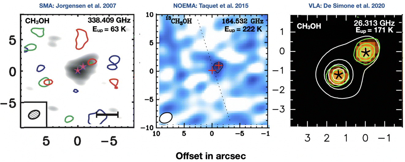 | ||
| Fig. 1 Images of the methanol line emission towards the solar-type protostar NGC1333 IRAS4A, obtained with three interferometers at different wavelengths. Left panel: SMA map in the submillimeter range (the gray image is the continuum emission, whereas the green contours show the CH3OH emission at the systemic velocity, and the red and blue contours at red-shifted and blue-shifted velocities, respectively).1Central panel: NOEMA map in the millimeter range (the image and contours show the CH3OH emission).2Right panel: VLA map in the radio range (the color image is the continuum emission whereas the white contours show the CH3OH emission).3 IRAS4A is a binary system whose two objects, A1 and A2, are indicated by stars (left panel), crosses (central panel) and asterisks (right panel). | ||
In this review, I will try to lay down the observational scenario of the early stages of the solar-type star formation, focusing in particular on the class of species called interstellar complex organic molecules, here called interstellar complex organic molecules (iCOMs),5,6 and the challenges that they represent to our current knowledge. Since their formation and destruction strongly depend on the formation of the ices that envelope the interstellar grains during the star and planet formation, the review will also briefly cover this aspect. Of course, this is only one part of the astrochemistry field. I chose to restrict this review because trying to discuss everything would end in discussing nothing in sufficient detail, so I decided to focus on something precise, choosing one of the currently most active fields of astrochemistry. Even with such a restriction, this review will be far from exhaustive so I will try to emphasize the most recent advances and challenges on the subject. I forward the interested reader to other recent reviews on the subject of astrochemistry during solar-type star and planet formation, where also different aspects and opinions are reported.7–12
Since this Faraday Discussion conference gathers together chemists and astronomers, I will try to have an interdisciplinary language understandable by the two communities, which may seem simplistic to either of the two communities at times, but I hope that in this way we understand each other on all the points discussed in this review.
Following this approach, this review will first summarise the overall framework of the solar-type formation process, with its major components and their physical and chemical characteristics (Section 2). I will then review the major observational characteristics of iCOMs during the solar-type star formation and in its different objects, with emphasis on recent high spatial resolution observations (Section 3). Third, I will discuss the major chemical processes occurring at each step and the critical quantities that regulate them, with the aim to emphasize what we do not know yet more than what we do (Section 4). In the subsequent section, I will provide some specific examples, with the goal of indicating what we can extract by comparing astronomical observations with the present astrochemical knowledge (Section 5). Finally, I will list the major conclusions and the take-home messages (Section 6).
2 From a molecular cloud to a planetary system
The process that leads the diffuse matter of a molecular cloud to form a solar-type star and its planetary formation, is long and complicated. At present, we have an overview of what we think happens, but several, even critical, passages are still obscure, as we will see in this review. That said, from a chemical point of view and for the context of this Faraday Discussion, four major phases can be identified, also corresponding to major changes and events in the physical processes and structure of the matter. Please note that previous reviews7–12 exist on the same argument by several authors and with more details, depending on the review focus, so that here I just briefly emphasize the points important to understand the chemistry. The four phases identified here are schematically shown in Fig. 2, while the physical parameters of the objects of each phase are summarised in Fig. 3. In the following sub-sections, I briefly describe them.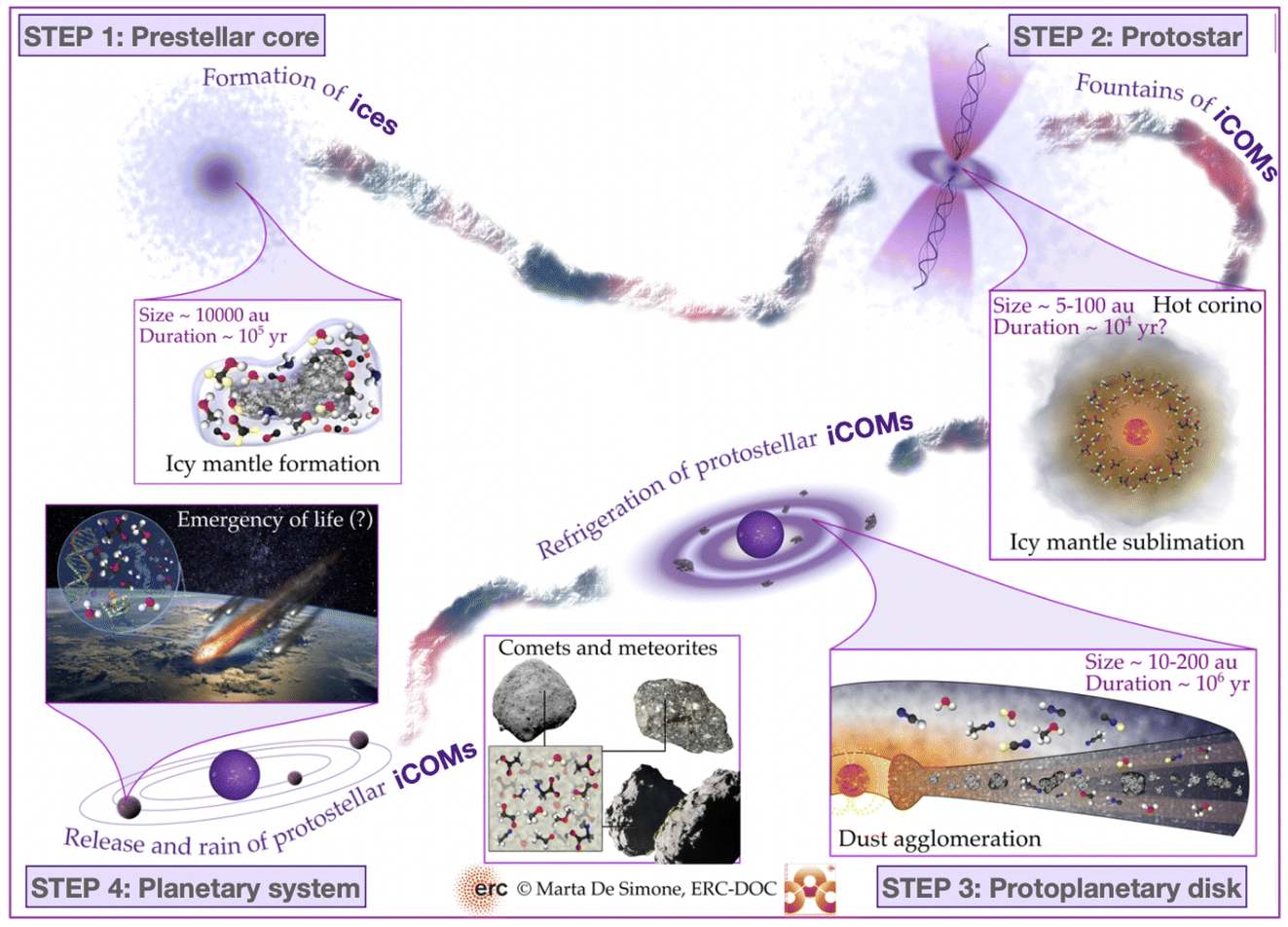 | ||
| Fig. 2 Sketch of the four major steps involved in the formation of a solar-type planetary system and its iCOMs (courtesy of M. De Simone), as described in the text. Step 1: In the cold (≤10 K) and dense (≥105 cm−3) prestellar cores, ices are formed on the surface of the interstellar grains. Step 2: In the hot corinos of and shocks surrounding, young protostars, iCOMs are observed in large quantities. Step 3: In protoplanetary disks, the hot corino iCOMs are frozen into ices enveloping the grains. Step 4: The dust grains coagulate into pebbles and larger rocks that will eventually become planets, asteroids and comets; some of the ices fabricated in steps 1 and 2 are in this way transmitted to the final planetary system. | ||
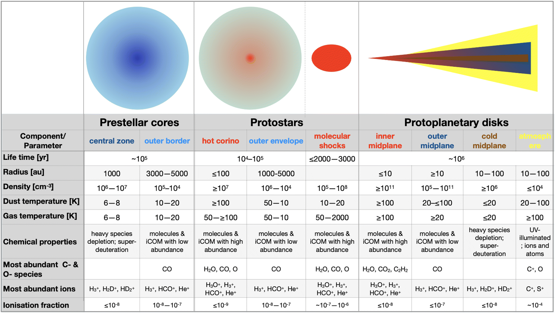 | ||
| Fig. 3 Physical and chemical properties of the objects of the first three phases of the solar-type star and planet formation, as described in the text (Section 2): prestellar cores, protostars and protoplanetary disks. The values in the table are rough estimates to provide orders of magnitude rather than precise estimates, which depend on the specific object of study. | ||
2.1 Phase 1: prestellar core phase
The story starts from a dense clump of material in a molecular cloud of the Galaxy. Under the gravitational force, which is contrasted by the hydrostatic pressure, the presence of magnetic fields and the turbulence in the gas, matter slowly accumulates towards the clump center. The clumps that have enough mass to eventually overcome all forces acting against the gravitation are called prestellar cores (PSC).Typically, PSC have a radius of ∼5000 au, a centrally condensed density structure, with the innermost part (≤1000 au in radius) flattened at a density of 106–107 cm−3, as summarised in Fig. 3. The temperature, in contrast, decreases towards the center: it is 10–20 K at the border of the PSC and decreases to 6–8 K at its center. The large density (with respect to the 104 cm−3 parental molecular cloud) and low temperature across the PSC have very important “chemical” consequences. First, the formation of thick icy mantles around the dust grains; second, the disappearance in the inner 1000 au region of gaseous CO and, more generally, any species containing elements heavier than H and D; third, an increase of the molecular deuteration of all species formed in this stage, either in the gas or on the grain surfaces.
2.2 Phase 2: protostellar phase
Once the gravitational collapse starts, a protostar is formed, consisting of one or more central objects (the future stars), their circumstellar disks (with radii of ≤100 au), a possible circumbinary disk (radius ∼100–1000 au) and an extended envelope (radius ∼300–5000 au). Since the gravitational energy of the infalling material is ultimately released at the center of the protostar, the temperature increases from 10–20 K at the envelope outer border to ≥100 K in the central (typically) ≤100 au region. Likewise, the density increases towards the center.While infalling, matter also rotates and, thus, to eventually accrete into the future star(s), it has to loose its angular momentum. This happens via the creation of the above-mentioned disks and the ejection of a substantial fraction of material, through what are known as jets and molecular outflows. On the other hand, the accretion of the matter from the rotating-infalling envelope towards the center likely proceeds in two major steps: trough large scale (∼100–1000 au) streamers of material crashing onto the disk(s) and from the disk(s) onto the central objects. Both the ejected and the streaming material create shocks when they encounter the quiescent one, in the envelope and disk(s).
From a chemical point of view, the envelope can be divided in roughly three zones. Starting from the border and going inward they are: (i) the outer border, which is similar to PSC (as it is its evolution); (ii) the lukewarm envelope, where some species such as CO and CH4 are desorbed from the grain mantles and reappear in the gas-phase; (iii) the hot envelope, where the dust temperature exceeds ∼100 K and the entire (or most of the) mantle is sublimated, releasing all the frozen species in the gas-phase. This region is called the hot corino if it contains iCOMs. Please note that Fig. 3 only summarizes the physical and chemical parameters of the hot corino and the outer envelope, for simplicity.
In shocked regions, the gas temperature and density increase with respect to the quiescent gas, by a factor that depends on the velocity of the shock. Typically, temperature increases up to a few hundred K and density to 105–108 cm−3 in molecular shocks around solar-type protostars. Despite the dust remaining cold (at about 10–20 K, as the shock is inefficient to heat it), frozen species are released into the gas-phase, either because of the sputtering or mechanical destruction of the grain mantles.
2.3 Phase 3: protoplanetary disk phase
With time, the protostellar envelope dissipates and the circumstellar disk, now also called protoplanetary disk, appears surrounding an older protostar, a pre-main-sequence (PMS) star. The disk is exposed to the photons of the central PMS star and the interstellar radiation, which has consequences on the disk structure and chemical composition. First, the disk is flared, that is, its thickness increases with the radius. The disk density in the midplane increases inwardly, reaching ≥1011 cm−3 in the inner 10 au zone, while it decreases going horizontally away from the midplane. Likewise, the temperature increases going inward and upward.From a chemical point of view, the disk can be divided in three zones: (i) the atmosphere, directly exposed to the UV, is similar to the PDRs (photo-dissociation regions) that surround the molecular clouds where atoms and ions dominate; (ii) the molecular layer, where several molecules are in the gas-phase, similar to the protostellar lukewarm envelope, but where UV photons may still have a role; (iii) the midplane, where chemistry is sort of similar to that in the protostellar envelopes: heavy-element bearing species are mostly frozen-onto the grain mantles in the outer zone (similar to the outer envelope), molecules are in the gas-phase in the intermediate zone (as in the lukewarm envelope), and mantles entirely sublimate in the inner midplane (as in the hot inner envelope). Note, however, that the icy mantles in the midplane also contain the new molecules formed in the prestellar and protostellar phases, even though it is not clear in what fraction. Mutatis mutandis, the chemistry in the circumstellar and circumbinary disks present in the protostellar phase is similar to that described here, except that these disks are surrounded by the envelope and, therefore, are less exposed to the UV photons.
That said, two important differences exist between the protostellar envelope and protoplanetary disk chemistry. First, the protoplanetary disks are thinner than the envelopes, and their chemistry is impacted more by the presence of UV photons, which are scattered across the molecular layer although not enough to photo-dissociate molecules. Second, the sizes of the dust grains hugely evolve with time: at the beginning the average grain radius is approximately ∼0.1 μm as in molecular clouds, while at the end of the protoplanetary disk evolution, dust grains become planets, asteroids and comets, as described in the next phase. In between, roughly speaking, grains in the midplane coagulate and migrate inward and outward, whereas grains out of the plane fragment and migrate vertically.
2.4 Phase 4: planetary system formation and heritage
As said, grains in the disk midplane coagulate and grow until they become the seeds of giant gaseous planets, rocky planets, asteroids and comets. This evolution is not completely understood, but obviously it happens. Currently, we think that it occurs via four major steps: (i) interstellar grain coagulation into pebbles of ∼10 cm; (ii) coagulation of pebbles into planetesimals of ∼1 km; (iii) formation and migration of giant planets; (iv) formation of rocky planets, asteroids and comets.From a chemical point of view and in the context of this Faraday Discussion, two major processes are important. First, the coagulation of the interstellar grains enveloped by the icy mantles formed during the previous three phases means that some of these ices are trapped in the interior of the pebbles and planetesimals, and so are protected. They constitute the heritage of the earliest phases of the planetary system formation. For example, water may be brought to the nascent planet by the rocky bricks that constitute it, as in the case of Earth.13–15 More in general, the trapped ices may be conserved almost intact in the interior of the most pristine bodies of the planetary system, as in the case of solar system comets.
Second, the composition of the formed giant planets depend on their position in the disk, as the major carriers of the elements (e.g. H2O, CO and CO2 for O, or N2 and N3 for N, etc.) are frozen in different zones of the disk midplane. In principle, this can be used to pinpoint where a solar and/or extra-solar giant planet has formed in the disk, despite it now being at a different position because of the planet migration.11,16 In practice, this is probably more difficult to obtain for the various uncertainties involved in the whole process,17 some of which regard chemical properties, principally the binding energies of the various species (see below).
3 Observations of iCOMs and ices in solar-type star forming regions
iCOMs are here defined as species with at least six atoms of which at least one carbon and another heavy-element, such as O, N, S and so on. iCOMs represent a special class of the almost 300 detected interstellar species, because of their potentiality of being precursors of prebiotic molecules. For this reason, since their first detection in the 70s they have aroused curiosity and interest, and, at the same time, have started a decade long quarrel on how iCOMs are synthesised in the harsh conditions of the ISM. After all these years, there is still no consensus. This is also the reason why this review focuses on iCOMs.In the following, I will summarise the observations towards the objects that represent different evolutionary stages or important components of the solar-like star formation process, emphasizing, when relevant, the high spatial resolution observations.
3.1 The cool chemistry in prestellar cores
Nowadays, we think we have understood reasonably well why this happens. In cold molecular gas, D is largely locked into HD. The most important way to “extract” D from HD and pass it to other species is via the reaction of HD with H3+, the most abundant ion (which is created by a chain of reactions started by the interaction of cosmic-rays with H2). Once every three times H2D+ is formed. Of course, H2D+ reacts back with H2 and, in the absence of peculiar conditions, the H2D+/H3+ abundance ratio is equal to 1/3 the elemental D/H. However, given the different zero point energy (∼230 K) of H2D+ and H3+, the H2D+ + H2 reaction, in cold enough gas, is much slower than the H3+ + HD one. This causes the H2D+/H3+ abundance ratio to be enhanced with respect to the elemental D/H. Then, the species formed from H2D+ and H3+ will inherit the D/H enhancement. This is the case for H2CO and its D-isotopologues (see later).
We have already seen that the temperature is very low in PSC, which is the first reason why the observed D2CO/H2CO abundance ratio in PSC is high. In addition, given the PSC low temperatures and large densities, CO, the most abundant gaseous neutral species in molecular clouds, freezes onto the dust grain surfaces disappearing from the gas-phase. Since CO is a major route of destruction of H3+, its disappearance from the gas-phase makes the destruction route of H3+ towards H2D+ increase, further enhancing the H2D+/H3+ abundance ratio.
In summary, any large molecular deuteration has origin in the prestellar phase. As we will see later in more detail, some iCOMs (and other molecules) in warm environments, such as hot corinos and shocks, are observed to have high D/H ratios. Since the temperature in these objects is too high for the deuteration to be a present day product, their high D/H ratio is indeed inherited, in one way or another, from the PSC phase.
While now there is no doubt on the presence of iCOMs in PSC, it is important to pin down where their line emission comes from, both for correctly estimating their abundance and understanding their formation mechanism. Vastel and collaborators, based on a non-LTE radiative transfer analysis, argued that the bulk of the methanol line emission in L1544, the most studied PSC, originates in the cold (∼10 K) and less dense (∼2 × 104 cm−3) gas at the border (∼8000 au from the center) of the condensation.24 Methanol line emission maps towards the same source confirmed that it does not come from the core itself but rather from the outer part of the L1544 condensation, less dense and exposed to weak UV illumination.25,29 This analysis has been done for methanol only, but it is more than likely that the other iCOMs also originate in the skin of the PSC, a hypothesis strengthened by the observations of other iCOMs in the methanol peak of L1544.26
The location of the detected iCOMs means that it is very difficult to estimate their absolute abundance, as the H2 column density is usually evaluated from the dust continuum emission, which only gives the integral towards the line of sight. Thus, if iCOMs are located in only a part of the line of sight probed by the dust emission, the derived abundance is a lower limit. Therefore, the most reliable quantity is the abundance ratio with respect to another species which emits in the same region. Usually, methanol, which is the most abundant iCOM, is taken as reference. Then, the survey of methanol and acetaldehyde carried out by Scibelli and Shirley,28 of more than two dozen PSC in the Taurus Molecular Cloud, the largest PSC sample so far, indicates that [CH3OH]/[CH3CHO] abundance ratio is about 10, within a factor of 5 (Fig. 4) (see also ref. 30). The measurements of L1689B estimate an abundance of methyl formate similar to that of acetaldehyde and about three times larger than dimethyl formate.20 As an indication, in L1544, Vastel and collaborators suggest a methanol abundance (with respect to H2) of ∼6 × 10−9.24Table 1 summarises the estimated abundances, with respect to methanol, of the iCOMs so far detected in PSC.
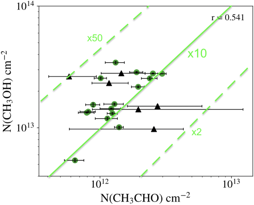 | ||
| Fig. 4 Column density of methanol (y-axis) and acetaldehyde (x-axis) measured in prestellar cores (black circles with their error bars).28 The green lines show the ratio [CH3OH]/[CH3CHO] equal to 10 (solid line) and multiplied and divided by a factor of 5 (dashed lines). | ||
| Name | Formula | [X]/[CH3OH] | |
|---|---|---|---|
| Prestellar cores | Hot corinos | ||
| Methanol | CH3OH | 1 | 1 |
| Acetaldehyde | CH3CHO | ∼0.1 | ∼0.1 |
| Ethanol | CH3CH2OH | — | 0.01–0.1 |
| Glycolaldehyde | HCO(CH2)OH | — | 0.001–0.01 |
| Methyl formate | HCOOCH3 | ∼0.01 | 0.01–0.3 |
| Dimethyl ether | CH3OCH3 | ∼0.003 | 0.003–0.1 |
| Formamide | NH2CHO | — | ∼0.01 |
| Methyl cyanide | CH3CN | 0.001–0.1 | 0.003–0.03 |
3.2 Chemical richness of the hot corinos in young protostars
| Source | Cloud (distance) (pc) | L bol (L⊙) | Class | First detection references |
|---|---|---|---|---|
| IRAS 19347 + 0727 (B335) | Barnard 335 (∼100) | ∼1 | 0 | 31 |
| IRAS16293-2422 A | ρ-Ophiuchus (∼140) | ∼20 | 0 | 32–34 |
| IRAS16293-2422 B | ρ-Ophiuchus (∼140) | ∼20 | 0 | 32–34 |
| L1551-IRS5 | Taurus (∼140) | ∼35 | I | 35 |
| BHR71-IRS1 | Coalsack (∼200) | ∼13 | 0 | 36 |
| IRAS 18148-0440 (L483) | Aquila Rift (∼200) | ∼13 | 0 | 37 |
| Barnard 1b-S | Perseus (∼300) | ∼0.3 | 0 | 38 |
| Barnard 1-a | Perseus (∼300) | ∼1 | I | 39 |
| Barnard 1-c | Perseus (∼300) | ∼1 | I | 36 |
| NGC1333 IRAS 1A | Perseus (∼300) | ∼3 | I | 36 |
| NGC1333 IRAS 4A1 | Perseus (∼300) | ∼6 | 0 | 40 |
| NGC1333 IRAS 4A2 | Perseus (∼300) | ∼6 | 0 | 40 |
| NGC1333 IRAS 4B | Perseus (∼300) | ∼6 | 0 | 41 |
| NGC1333 IRAS 2A1 | Perseus (∼300) | ∼16 | 0 | 41 |
| NGC1333 SVS13-A | Perseus (∼300) | ∼32 | I | 42 and 43 |
| L1455 IRS 1 | Perseus (∼300) | Unknown | I | 36 |
| IC 348 MMS A | Perseus (∼300) | Unknown | I | 36 |
| Per-emb 26 | Perseus (∼300) | Unknown | I | 36 |
| HH 212 | Orion (∼400) | ∼9 | 0 | 44 and 45 |
| HOPS-108 | Orion (∼400) | ∼38 | 0 | 46 |
| MMS6 | Orion (∼400) | ∼ | 0 | 47 |
| CSO33-b-a | Orion (∼400) | ≤23 | 0 | 48 |
| SIMBA-a | Orion (∼400) | ∼2 | 0 | 48 |
| FIR6c-a | Orion (∼400) | ∼8 | 0 | 48 |
| MMS9-a | Orion (∼400) | ∼9 | 0 | 48 |
| MMS5 | Orion (∼400) | ∼16 | 0 | 48 |
| Ser-emb 1 | Serpens (∼440) | ∼4 | 0 | 49 |
| Ser-emb 17 | Serpens (∼440) | ∼4 | I | 50 |
| Cep E-B | Cepheus (∼800) | ∼75 | 0 | 51 |
By far the best studied hot corinos are those in the protobinary system of IRAS26293-2422, where just over a dozen iCOMs have been detected.32–34,54,57–61 In contrast, just a few iCOMs have been detected in other hot corinos. Table 1 summarises the iCOMs detected in at least three hot corinos and their abundance relative to methanol.
Recent observations have also taught us that the detection of hot corinos and iCOMs can be dramatically hampered by the wavelength used for the observations and, therefore, the picture that we may derive from them. The figure shown at the beginning of this review (Fig. 1) illustrates this problem. Methanol towards the south source, IRAS4 A1, is only detected when observed in the radio range. In addition, the intensity of the methanol lines is very similar to that emitted by the north source, IRAS4 A2, the only one of the two detected in the mm, suggesting that the two hot corinos have likely similar iCOMs abundances. Therefore, restricting the observations to the mm range would have given a very different scenario: two very close siblings would have very different chemistry, a puzzle and challenge for astrochemical models…which indeed it is not. The reason for the above behavior is the absorption of the dust mixed with the gas in front of the hot corinos, which are embedded in the envelopes. Since the dust absorption efficiency decreases with increasing wavelength, it blocks the hot corino line emission in the submm and mm range, whereas it becomes transparent in the radio range. Therefore, it can be dangerous to limit the observations to the submm and mm wavelength ranges, because they may give a wrong picture and wrong iCOM abundances.
However, the dust absorption can also have a beneficial effect: to reveal the spatial stratification of the iCOM in a hot corino, even in the absence of the spatial resolution that would be required to resolve the line emission from different iCOMs. This is what has been observed so far in at least two objects, SVS13A and HH212-mm. The effect and principle is illustrated in Fig. 5.
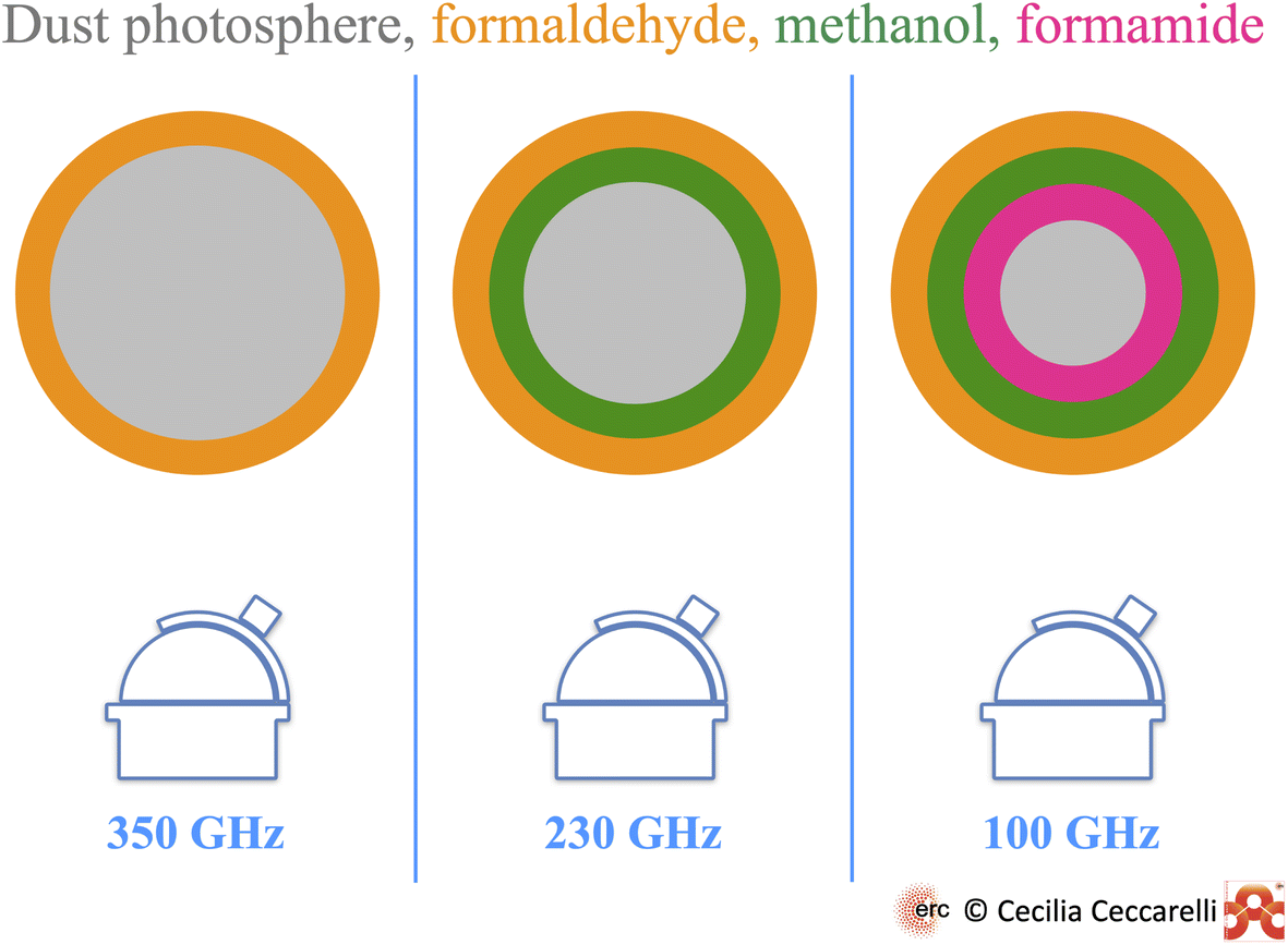 | ||
| Fig. 5 Sketch of the combined effect of dust optical depth and iCOM binding energy (BE) on the iCOM detection towards the NGC1333-SVS13A hot corino over a 45 au scale.62 Observations at 350 GHz (left panel) can only detect formaldehyde, whose BE allows it to be present over almost the entire envelope. Observations at 230 GHz (middle panel), where the dust optical depth is smaller than at 350 GHz, can also detect methanol, whose BE is larger than that of formaldehyde. Finally, observations at 100 GHz (right panel) can penetrate the most through the envelope, because the dust optical depth is the lowest and, therefore, detect formamide whose BE is the largest. | ||
Until very recent, only “simple” deuterated molecules were observed, with the most complex being methanol. These molecules are either formed in the gas phase directly via reactions with H2D+, such as DCO+ or N2D+, or indirectly. Even in species formed on the grain surfaces, such as water and methanol, the deuteration originates from the enhanced H2D+/H3+ abundance ratio, which regulates the D/H atomic abundance in the gas and, hence, landing on the grain surfaces (see Section 4.2.2).
With the advent of the high sensitivity of ALMA and the very successful survey PILS,59 deuterated iCOMs have also been detected: formamide, acetaldehyde, dimethyl ether, methyl formate, glycolaldehyde, ethanol and methyl cyanide.43,66–71 The detection and abundance determination of deuterated iCOMs is important because it has great diagnostic power to discriminate the route of formation of the species, if predictions can be obtained for the different routes of formation, as will be explained in Section 5. In general, organics show a deuterium fractionation of about 1–10%, larger than that measured in water (≤1%) towards the same sources, likely reflecting the history of the ice formation: water first, iCOMs later.8
Another application of the fact that prestellar ices are injected into the gas-phase is that their abundance can be used to constrain the prestellar core ice formation.72 It is important to emphasize that we actually do not observe ices in the prestellar cores, because, as the ice observations are from absorption in the IR wavelength, we would need a strong IR source behind the prestellar core. While JWST will provide a huge amount of data on the ices in molecular clouds, it will not be able to sample the central zones of the prestellar cores, where the ices that govern the hot corino chemistry are formed. A first study towards the IRAS4a and IRAS4B hot corinos of two major ice components, methanol and ammonia, injected into and observed in the gas-phase, seems promising.72 It suggests that the prestellar ice formation of these two objects was abruptly interrupted by the clash of an expanding bubble, coming from a distant and ancient supernova explosion, against the molecular cloud to which IRAS4a and IRAS4B belong. However, in order to extract this information, the observations have been compared with astrochemical model predictions which may or may not be reliable enough for the clash suggestion to be confirmed.
3.3 Shocks during star and planet formation
As mentioned in Section 2, the accretion process during the protostellar phase is accompanied by supersonically ejected or infalling material that crashes against quiescent matter, causing the so-called molecular shocks, where numerous and abundant molecules are observed. The shocks from outflowing matter have been known and studied for decades, and are called protostellar outflow shocks, while the discovery of streamers of material falling into the circumbinary or circumstellar disks and creating shocked regions is more recent (see also the contribution by Bianchi et al. in this volume).73–75 At the moment of writing this review, very little is observationally known about the chemistry of the shocks caused by the infalling streamers, so in the following, I will focus on those caused by the protostellar outflows.Despite the phenomenon of the outflows being known since the 80s and dozens of protostellar outflows studied in CO, in only two cases have iCOMs other than methanol been detected so far: the shocked region called L1157-B1 and the shocks caused by the outflows emanating from the IRAS4A binary system (mentioned in the Introduction). In both shocked regions, the “usual suspect” iCOMs have been detected: methanol, acetaldehyde, methyl formate, dimethyl ether, glycolaldehyde and methyl cyanide.
Fig. 6 shows an illustrative and important example, that of the deuterated formaldehyde, acetaldehyde and formamide line emission maps observed towards L1157-B1. The emission of deuterated formaldehyde clearly shows the regions where grain mantle species, previously formed in the cold phase, have been recently injected into the gas-phase. Acetaldehyde emission is overlapped, signalling a fresh release from the grain mantle too, whereas that of formamide is slightly but definitively displaced towards the south, where the dynamics of the region indicate an earlier passage of the shock. This example is illustrative because it shows that high-resolution maps of iCOMs provide the history of the shock passage and the evolution of chemistry: in particular, unless the ices are substantially different in the two regions where acetaldehyde and formamide are seen, the displacement means that formamide is a late product formed in the gas-phase from and after the injection of the ice components. It is important because this information provides an additional and precious constraint to the astrochemical models, in addition to the measured abundance and abundance ratios: how species evolve with the time. We will see later, in Section 5.2, how this information can help to constrain the formation route of formamide in this source.
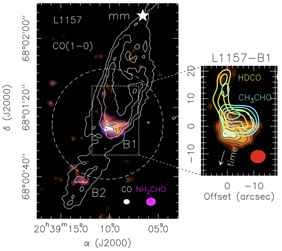 | ||
| Fig. 6 Images of deuterated formaldehyde, acetaldehyde and formamide towards the shocked region of L1157-B1, in the southern lobe emanating from L1157-mm. Left panel: map of CO (1–0) line emission (white contours)76 that shows the overall morphology of the outflow, where several clumpy cavities are excavated by the precessing jet, the brightest of which is B1. The color map shows the formamide line emission.44 The dashed circle indicates the primary beam of the NH2CHO image, namely the field of the observations. The magenta and white ellipses depict the synthesised beams of the CO (white) and formamide (magenta) observations. Right panel: map of the line emission of HDCO (yellow contours),77 acetaldehyde (cyano contours)44 and formamide (color image).44 The region where HDCO emits shows where the grain mantles were recently sputtered by a shock. The region where HDCO does not emit but molecular emission is still visible is a region where a shock hit earlier. Therefore, the displacement between acetaldehyde (region coincident with the HDCO emitting one) and formamide (south region with no HDCO and CH3CHO emission) is due to the time lapse between the two shocks. | ||
3.4 The hidden chemistry in protoplanetary disks
Observations of molecules in protoplanetary disks has been a decades long and painful hunt, where astronomers have struggled even to observe the simplest species. This is because protoplanetary disks are small in size and the molecular emission originates in the molecular layer described in Section 2.3, which has a relatively low column density. The advent of ALMA has greatly improved the situation providing the first detection of iCOMs in the outer regions of the disks and the first images of snow lines.35,78–81 However, even methanol turns out to be a species difficult to detect in protoplanetary disks,82 maybe because of the large dust opacity that absorbs much of its emission83 or the relatively low temperature.84 Fortunately, the new observations of JWST are already giving plenty of information on the inner regions of the disk,85–87 an appetizer of which is also reported in this volume (e.g., van Dishoeck et al. and Kamp et al.).So far, the disk with the largest inventory of detected iCOMs is HH212-mm, a very young disk in the Orion region.45,88–90 Once again, the usual iCOMs suspects are detected: methanol, acetaldehyde, methyl formate, formamide and methyl cyanide. This is another interesting case where observations at different wavelengths reveal the stratification of iCOMs in this disk due to the difference in the species binding energies91 (Fig. 7). Actually, observations at different wavelengths could even be used to infer the succession of the binding energy of different species.
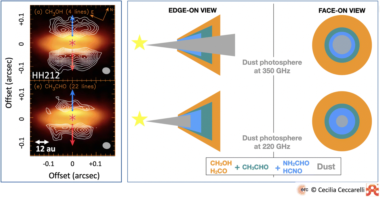 | ||
| Fig. 7 iCOMs in the disk surrounding HH212-mm. Left panel: images of the methanol (top) and acetaldehyde (bottom) line emissions (white contours) overlapping the dust continuum emission (in color).90 Note the lack of molecular line emission on the plane of the disk, which is seen almost edge-on, because of the absorption of the dust, giving it a hamburger-like shape. Right panel: sketch of the line emission from iCOMs and other species detected toward the disk: methanol, formaldehyde, acetaldehyde and fulminic acid. The regions where each species is detected at ∼350 GHz (upper panels) and ∼220 GHz (lower panels) are shown with the disk edge-on (left panels) and face-on (right panels) along with the dust photosphere. The molecular line emission depends on the combination of the wavelength at which each species is observed, and its binding energy. For example, methanol is only in the upper atmosphere if observed at 350 GHz, whereas it appears over the whole disk if observed at 220 GHz. | ||
Another very promising disk is the one in the FuOri star V883. This source has recently undergone a burst in its luminosity. The burst was first announced in 1888 (but not measured) and, later, a bolometric luminosity of ∼400 L⊙ was measured.92–94 The luminosity has been decreasing in the past years to a present value of 218 L⊙.95,96 The interesting point is that the sudden increase of the luminosity causes the heating of the dust at a larger distance from the center than in the quiescent status. In the region where the temperature exceeds that of water ice sublimation (∼120 K, which correspond to a radius of about 320 au in the case of V388), iCOMs trapped in the ice are injected into the gas-phase, like in the hot corinos (Section 3.2), and become observable along with water.97–101 Not surprisingly, the detection of methanol, acetaldehyde, methyl formate and methyl cyanide have been reported.98,99
3.5 Interstellar ices
While the discovery of ices enveloping the interstellar dust grains dates back to the 70s, the revolution in this field started with the advent of the first spatial telescope, the ESA satellite ISO (Infrared Space Observatory), which provided spectroscopic observations in the infrared (IR) of hundreds of sources. Two other space-borne telescopes followed, Spitzer and AKARI, to complete that first revolution. These observations have provided the inventory of the most abundant species present in the ices: H2O, CO, CO2, NH3, CH4 and CH3OH. Other species, such as H2CO, are less abundant and not always present. The review by Boogert and collaborators102 offers an excellent view of what has been learned so far.Important in the context of this review is when ices start to appear and with what composition. Water is the first solid species appearing already in molecular clouds with a visual extinction of ∼3 mag, meaning at a cloud depth of ∼1.6 mag (as the cloud is UV irradiated on both sides). Solid CO2 is also detected in molecular clouds starting from a visual extinction of ∼3 mag, with an abundance with respect to H2O of ∼15–40%. Solid CO appears at ∼6 mag with an abundance of ∼10–70%, followed by CH3OH at ∼18 mag with an abundance from ≤1 up to ∼12%. Ammonia and methane are not detected towards molecular clouds with upper limits of ∼5%.
In denser protostars, the abundance of solid CO2 and CO (relative to H2O) is similar to that measured in molecular clouds, whereas that of solid methanol is up to two-times larger, and methane and ammonia is only about ∼1–10%. In practice, when considering the uncertainties, only methanol seems to be more abundant in the line of sight of dense envelopes of protostars than in those of molecular clouds.
Today we are at the verge of a second revolution thanks to JWST, which has unprecedented sensitivity and spectral resolution in the IR. A first work by McClure and collaborators103 has provided a very appealing appetizer of what awaits. These authors presented observations towards two field stars, probing ices in the solar-type star forming region Chameleon I, in front of them. In addition to the most abundant and known species, the obtained spectra suggest the presence of less abundant species, notably ethanol, even though the detection is not confirmed. In addition, the high JWST sensitivity has allowed the observations of many more sources in the line of sight, which will provide a relatively high resolution map of the ice composition across the studied molecular cloud, the first ever. In the same vein, JWST observations by Yang and collaborators toward the envelope of a young protostar,104 show the presence of the usual ice components and spectroscopic features that could be attributed to ethanol and, maybe, acetaldehyde.
4 Chemical processes and quantities
As we all know, having good and reliable observations is necessary but not sufficient for progressing our knowledge, namely in understanding what happens and why. For that, we need models, in our specific case astrochemical models. One can think of models as boxes that contain processes and quantities, which make a theory, and work them out into predictions that are, finally, compared with observations. When the model predictions are able to reproduce the observations, the model and, thus, the theory are validated.In general, astrochemical models need two classes of information: one relative to the physical and chemical properties of the object to be modeled and the second to the chemical processes occurring in the ISM conditions and the quantities associated with them (Fig. 8). In the next two sections, I briefly review how the object’s physical and chemical properties are generally extracted from the observations and the chemistry of iCOMs, respectively.
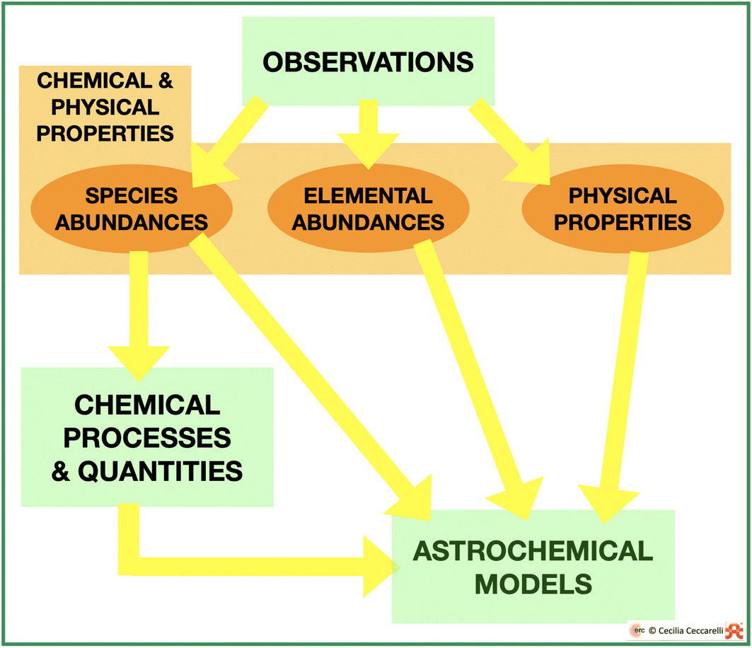 | ||
| Fig. 8 Sketch of the input of astrochemical models. Astronomical observations provide an object’s chemical and physical properties, namely the detected species and their abundance, the elemental abundances and physical parameters (density, temperature and so on). The observed species provide the input to ascertain the chemical processes and quantities. Finally, all information is combined to create the astrochemical models. | ||
4.1 Inputs of the astrochemical models
The first one is that in order to have a reliable radiative transfer model one needs the so-called collisional coefficients for the studied species. These coefficients are usually obtained via quantum mechanical (QM) computations, because experiments of the state-to-state excitation are extremely difficult and have been obtained for very few species.105–109 In the case of iCOMs, only the methanol and methyl cyanide have available collisional coefficients: methanol for collisions with H2 (ortho and para) for the first 256 levels and temperature between 10 and 200 K;,110 methyl cyanide for collisions with He only, between 20 and 140 K and for J ≤ 25.111
The second source of uncertainty is the derivation of the species abundance, which requires knowledge of the H2 column density of the same region emitting the species lines. As already mentioned in Section 3, deriving the H2 column density is extremely difficult if not impossible, because the H2 first excited level is at ∼500 K and, therefore, the ground transition, by definition, only probes ≥50–100 K gas. In addition, as the transition is at 28 μm, observations can only be obtained with a space born telescope. JWST will provide new data in this respect, but, for the moment, the H2 column density is mostly indirectly derived from the continuum observations (which have themselves uncertainties in the conversion from the dust to the gas column density, about a factor 3).
Finally, a third source of uncertainty is the inevitable approximation of the 3D structure of the studied object, because we only have 2D observations. Often, for an astronomer “the cow is a sphere”, to say that a simple (e.g. spherical) symmetry is often assumed (for disks it would be cylinder symmetry, a slab for a cloud and so on). This is important to keep in mind because the estimates of the chemical abundances from observations have an uncertainty of, at least, a factor of three to be optimistic. Abundance ratios could be more reliable, if we have strong reason to believe that the two species originate exactly in the same region, which may not be the case even when the observations show them in the same line of sight (see, e.g., the discussion in Section 3.2).
Both carbon and oxygen are contained in the refractory component of the interstellar grains and in their volatile one. Oxygen is contained in silicates, while carbon is contained in so-called grains of carbonaceous material: a very difficult to characterize and quantify component of interstellar dust.113
In dense molecular clouds in the vicinity of the Sun, the sum of the abundances of gaseous and frozen CO, frozen H2O, CO2, CH4 and CH3O, and the oxygen trapped in the silicates should give a total equal to the elemental abundance measured in the Sun. Unfortunately, this is not the case and about one third of oxygen is “missing”, i.e. we do not know where it is.114,115 Please note that CO is measured to be the most abundant C- and O-bearing gaseous molecule in dense molecular clouds, with stringent measurements and upper limits of the H2O and O2 molecules, less abundant by at least a factor of 1000. However, we do not have straightforward measurements of atomic oxygen in cold molecular clouds, because of the difficulty of observing its ground line at 63 μm with adequate spectral resolution. In practice, very few observations exist and most were obtained by ISO. The ISO observations gave puzzling results, as they suggested that a substantial fraction of atomic oxygen could be gaseous.116–118 More recent observations obtained with the airborne telescope SOFIA toward a couple of massive sources, confirm the presence of a substantial fraction of atomic oxygen (∼10−5 with respect to H-nuclei) associated with molecular gas, but not enough to account for the missing elemental oxygen.119,120 Therefore, the missing oxygen could be in refractory material difficult to observe, as O-rich carbonates or oxidized metals.115
Carbon elemental abundance is also difficult to constrain, because of the difficulty of quantifying the amount of carbon locked into the dust grains.115
Needless to say but better to do it: the choice of the oxygen and carbon elemental abundance has a huge impact on the predicted abundances of iCOMs in any model.
4.2 iCOMs chemistry
The second class of information necessary to any astrochemical model regards the chemical processes and quantities: they are the precious engine of the models. This section presents an overview of what is known so far, what is not completely clear and, finally, what is still missing in our understanding of the formation of iCOMs.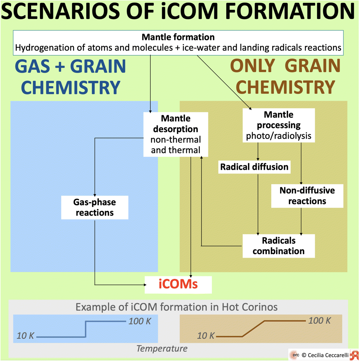 | ||
| Fig. 9 Sketch of the two major scenarios invoked in the literature for the formation of iCOMs: “Gas + grain chemistry” and “Only grain chemistry”. Both predict the formation of icy mantles enveloping the interstellar dust grains, prevalently during the cold molecular cloud and prestellar core stages. The mantle constituents are the result of the hydrogenation of atoms and simple molecules, such as CO, and the oxidation. Water and methanol, for example, are formed in this first step.121–123 In addition, after the first layers of water-ice are formed, radicals landing on the grain surfaces can react with the ice-water molecules. The iCOM ethanol, for example, can be formed in this way.124 After this first step, the two scenarios differ as follows. Left blue panel: In the “Gas + grain chemistry” scenario, the mantle components are either partially or completely injected into the gas-phase by thermal and non-thermal desorption processes, where they undergo gas-phase reactions that form iCOMs. This can occur either via mantle thermal desorption in hot corinos and inner protoplanetary disks, or via mantle non-thermal desorption in prestellar cores, outer protoplanetary disks and molecular outflows. Right brown panel: In the “Only grain chemistry” scenario, the icy mantles are processed by UV (photolysis) and CR (radiolysis) irradiation while being formed, and the radicals formed by the two processes remain trapped in the ice. When the dust temperature increases, radicals on the mantles become mobile and diffuse and, when they meet or meet some closed-shell species, they combine forming iCOMs. Alternatively, non-diffusive processes can also combine radicals into iCOMs. Likewise, some radicals are also predicted to meet and react in non-diffusive processes during the cold phase. | ||
However, the two scenarios diverge when other species are considered, especially iCOMs. Briefly, to give an illustrative example, let me consider the case of the iCOM formation in hot corinos. In the so-called “Gas + grain chemistry”, after the mantle formation, the frozen species are injected into the gas-phase when the dust grain temperature exceeds the water ice sublimation, ∼100 K. Once in the gas-phase, these species undergo a series of reactions that form iCOMs. In the other scenario, the “Only grain chemistry”, after their formation, mantles are processed by photolysis and radiolysis creating radicals that remain trapped in the ices. With the evolution of the protostar, the dust temperature gradually increases. When it reaches a temperature where the trapped radicals can migrate, the latter can encounter other radicals and combine into iCOMs, also radicals can combine with closed-shell species. Also, reactions not involving the thermal migration of radicals could also take place, most of them ending up in radical combinations of iCOMs. Finally, when the dust temperature reaches the ice sublimation, the iCOMs, synthesised on the grain surfaces, are released into the gas-phase where they are observed by submm/mm/radio telescopes.
In the following sections, I briefly review the status of our understanding of some of the processes involved in the iCOM formation along with the quantities that characterise them, following the scheme in Fig. 9.
In the following, we briefly summarise the process of formation of the firmly detected O-, C- and N-bearing ice components.
Water. We think we have a good handle on the process forming water on the ices – the hydrogenation of atomic and molecular oxygen, landing on the grain surfaces – based on experiments121 and quantum mechanics (QM) computations.125 This also agrees with water being formed very early in molecular clouds (from atomic rather than molecular oxygen).
CO2. The formation of CO2 has been studied in laboratory experiments and the community agree that it mainly occurs via the CO + OH reaction, which forms the HOCO radical (assumed to be excited) that eventually becomes CO2.126 There are no explicit QM computations that have simulated the process yet.
CO. Obviously, solid CO is due to CO formed in the gas-phase freezing onto the grain surfaces (which also implies that seeing a species on the ice mantles does not imply that it is formed there).
Methanol. Since the early 2000s, laboratory experiments have shown that methanol is formed on the water ice surfaces via addition of hydrogen atoms to frozen CO
![[thin space (1/6-em)]](https://www.rsc.org/images/entities/char_2009.gif) 122 (see also the review by Tsuge and Watanabe123). The idea is that the two steps with an activation barrier, CO + H and H2CO + H, are overcome by the H-atom tunnelling through them. Theoretical computations have been published later and confirmed the experimental results.127,128 The form of the barriers (height and width) and the consequent rate coefficient of methanol formation, differ in the studies by Rimola and collaborators127 and Song and Kästner,128 as the first refers to Eley–Rideal reactions while the second one to Langmuir–Hinshelwood. Unfortunately, most astrochemical models adopt a rectangular barrier, with the height and width derived from approximating gas-phase computations,129–132 predicting methanol formation rate coefficients more than four orders of magnitude smaller than the ones computed by Song and Kästner,128 for example.
122 (see also the review by Tsuge and Watanabe123). The idea is that the two steps with an activation barrier, CO + H and H2CO + H, are overcome by the H-atom tunnelling through them. Theoretical computations have been published later and confirmed the experimental results.127,128 The form of the barriers (height and width) and the consequent rate coefficient of methanol formation, differ in the studies by Rimola and collaborators127 and Song and Kästner,128 as the first refers to Eley–Rideal reactions while the second one to Langmuir–Hinshelwood. Unfortunately, most astrochemical models adopt a rectangular barrier, with the height and width derived from approximating gas-phase computations,129–132 predicting methanol formation rate coefficients more than four orders of magnitude smaller than the ones computed by Song and Kästner,128 for example.
Ammonia. Solid ammonia is formed by the hydrogenation of atomic nitrogen, a process that has recently been studied via QM computations.133 Later, ammonia formed in the gas-phase can also freeze-out onto the grain surfaces and enrich it further.72,134 The fact that ammonia is actually detected towards protostellar envelopes may suggest that this second route is not negligible.
Methane. For a long time it was believed that methane is formed by successive hydrogenation of atomic carbon, as also shown in a recent laboratory experiment,135 or by reactions with surface H2.136 However, recent QM studies are unanimous in showing that atomic carbon reacts with the water molecules of the ices and can not form methane.137–139 Likely, in the ISM, the H addition chain starts rather from gaseous CH landing on the ice surfaces. The methane example also shows the importance of having QM computations that describe the micro-processes occurring on the grain surfaces, to be able to include the correct processes.
Ethanol. Recent QM computations predict that ethanol can be formed on the grain surfaces by the CCH, formed in the gas-phase, which instantaneously reacts with one water molecule of the ice to form vinyl alcohol in a barrierless reaction, which can then be hydrogenated into ethanol.124
Minissale and collaborators have recently published a comprehensive review of the BE of about 20 species (including H, O and C atoms).140 Probably needless to say, the list does not contain any radicals. Also, only three iCOMs appear in the list: methanol, methyl cyanide and formamide. More recently, Ferrero and collaborators and Molpeceres and collaborators reported a joint experimental and theoretical study of the BE of acetaldehyde.51,141
An alternative means to obtain the BE of the species is via QM computations. Actually, this is probably the only way to obtain the BE of radicals. In the last few years, Ugliengo, Rimola and collaborators have carried out various QM computational studies and provided the BE of almost four dozen species, including radicals, iCOMs and S-bearing species.142,143 These BEs have been obtained using models for the ice containing 64 water molecules. In the same vein, Bovolenta, Bovino and collaborators have carried out QM computations of the BE of almost two dozen species on 22 water molecules of ice, among which are two iCOMs – methanol and formic acid.144,145 All these recent theoretical studies have highlighted an obvious point – adsorbed species do not have a single BE but a distribution of values, which depend on the species (where and in what orientation they land on the ice) and the adsorbate (e.g. crystalline or amorphous water ice, or CO-rich ice). However, this is overlooked by models with only one exception.146
In this respect, Tinacci and collaborators have obtained the most extensive QM study and complete distribution of BE, obtained for ammonia and water over a large ice grain of 250 water molecules.147,148 The example of the BE distribution of ammonia is reported in Fig. 10. The distribution is described by two Gaussian functions, which reflect the two possible H-bonds that the ammonia can form with water: the stronger the N⋯H(–OH) and the weaker N–H⋯O(H2), where the ammonia is respectively H-bond acceptor and H-bond donor.
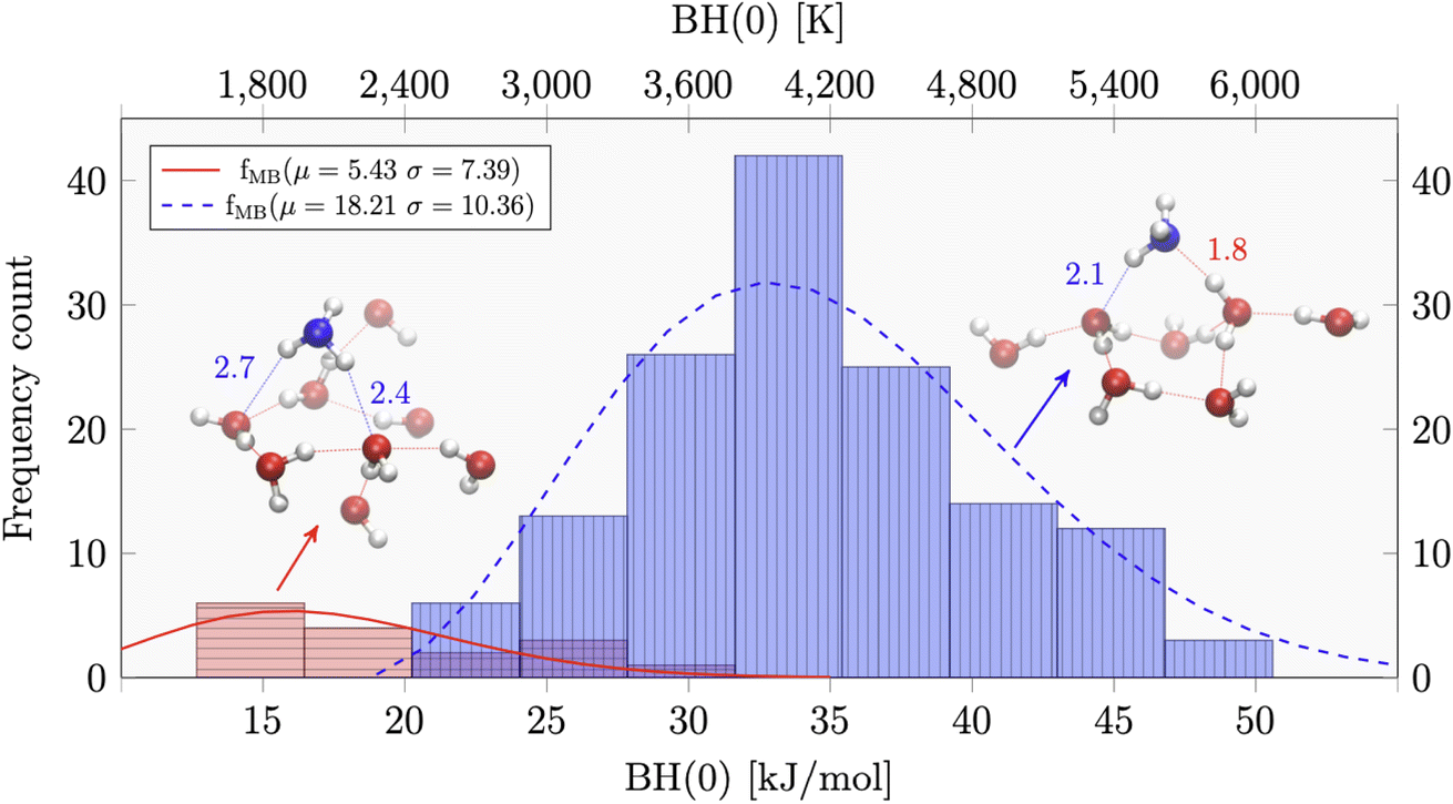 | ||
| Fig. 10 Distribution of the binding energy, which is the binding enthalpy corrected for the zero point energy BH(0), of ammonia adsorbed on amorphous water ice as derived by quantum mechanical computations.147 In these computations, the icy grain model constitutes 250 water molecules. The distribution can be fitted with two Gaussian curves, which reflect the two possible H-bonds that the ammonia can form with water: the stronger N⋯H(–OH) and the weaker N–H⋯O(H2), where the ammonia is respectively H-bond acceptor and H-bond donor, as shown in the figure. | ||
Finally, the other parameter entering in the astrochemical models to compute the sublimation temperature of a species, is the so-called pre-exponential factor. Usually, this is taken as a fixed number, ∼1012 s−1, but several studies have now emphasized the necessity to have this number coupled with the BE of the species.140,141 In other words, the ∼1012 s−1 may be very wrong for heavy molecules. For example, for acetaldehyde the pre-exponential factor is ∼1018 s−1. In this case, using ∼1012 s−1 would lead to a sublimation temperature of about 10–20 K different from the correct one.12
Present day gas-phase reaction networks contain more than 8000 reactions (more than double if D-isotopologues are taken into account) that involve about 500 (or more) species. Two major gas-phase networks are publicly available and used by several astrochemical models: KIDA†153 and UMIST.‡154 First, I would like to acknowledge the huge and heroic effort carried out by our colleagues that have first built the reaction networks on which the two above mentioned databases are based on, especially Eric Herbst and Tom Millar. That said, the KIDA and UMIST database networks suffer some problems that cannot be ignored, and which I here identify as reactions that (i) “should not be there because they are wrong” and (ii) “are missing”.
Reactions that should not be there. As indicated in the two databases, the large majority ≥80% of the included reactions has never been studied in laboratory experiments or by theoretical computations. Even in the cases of reactions that have been investigated, the experimental conditions rarely reproduce those typical of solar-type star forming regions, either regarding the temperature or the density. In the absence of laboratory data, rate coefficients and their temperature dependence are mainly estimated with some chemical intuition or by drawing analogies with similarly known processes. When the data are available outside the temperature or density range of relevance, they are used as such or are extrapolated. However, both approaches can be seriously wrong for various reasons, discussed elsewhere.12
One obvious error in writing down schemes of unknown reactions from similar arguments is that the formation enthalpy of the products may be larger than that of reactants, especially when unstable species, such as ions or radicals, or other uncommon species are involved. In this context, Tinacci and collaborators155 carried out systematic work to “clean” the gas-phase reaction network GRETOBAPE,§ which is based on the KIDA network, from the most obvious source of error: the presence of endothermic reactions not recognized as such. Using the enthalpy of formation derived by electronic structure calculations,156,157 these authors found that about 5% of the reactions in the original network resulted in endothermic reactions erroneously reported as barrierless or with too low activation energy. While on the one hand it is reassuring to know that the networks are not hugely wrong, one should not underestimate the impact of this 5% of erroneous reactions. For example, Tinacci et al. found that the overall silicon chemistry is hugely impacted by this.155
Other possible errors are the presence of reaction activation barriers which are either over- or under-estimated, wrong rate coefficients and wrong products. In these cases, dedicated experiments and/or QM computations are needed, which is extremely time consuming. The example of formamide that will be discussed later (Section 5) illustrates the difficulty of correcting the networks for relatively small, but still important in the interstellar context, activation barriers. Another example is provided by acetaldehyde, also discussed later (Section 5): about half of the acetaldehyde formation reactions listed in the KIDA database have either the wrong rate coefficient or products.158
Reactions that are missing. Despite the large dimensions of the available gas-phase reaction networks, there are no doubts that some important, and maybe also crucial, reactions are missing.
One obvious class of missing reactions are those in which neutrals react with the most abundant ions in molecular gas, namely HCO+, H3+, He+ and H+. Tinacci and colleagues reported that, out of 238 neutral species present in the GRETOBAPE network, 111 of them do not have reactions with at least one of the above-mentioned ions, and 10 not even with one ion.155
Finally, it is more than probable that important gas-phase reactions are missing. Some of them may even be present in the literature but just overlooked. One example is the formation of methyl formate from dimethyl ether which was only introduced in 2015 (ref. 159), although the chain of reactions were measured and computed since 2005. Another possibility is just that reactions were not thought of, like the case of the formation of glycolaldehyde, for which no gas-phase formation routes were present in the database or literature: ad hoc new QM computations showed that there exists at least one formation route of glycolaldehyde in the gas-phase.160
As said, both laboratory experiments and QM computations are very time consuming, so it is important that chemists and astronomers work together. It is possible that artificial intelligence (machine learning) techniques could help to reduce the burden. A recent work by Stancil and collaborators on the application of an artificial neural network to compute collisional excitation rate coefficients161 is very promising and perhaps a similar approach could be used for reactions. Another approach could also be the one recently applied by Komatsu and Suzuki,162 to automatically search for paths of formation of cytosine.
In Fig. 9, (at least) four processes are involved in the formation of iCOMs on the grain surfaces. They are briefly reviewed in the following.
Mantle processing. Once the “first generation” ice is formed (H2O, CO, CO2, NH3, CH3OH…), it is processed because of the UV illumination (photolysis) and/or cosmic-ray (radiolysis) irradiation forming radicals that remain trapped in the ice. To correctly describe the process and introduce it into astrochemical models, one needs to know what radicals are formed and at what rate. In the case of UV photolysis, models rely on the gas-phase reactions for introducing the products. While this may be correct, the possibility that the created radicals instantaneously react with the ice-water molecules and become something else, is mostly overlooked by models so far (see the cases of CN and CCH
124,164). For the radical production rates, models again use the ones from the relevant gas-phase reactions, sometimes applying adjusting factors.165 Unfortunately, while several experiments focused on the interstellar analogues photolysis, it is very difficult, if not impossible, for them to describe the microphysics process and, thus, estimate the radical production rates. One obvious reason is that the created radicals instantaneously react on the irradiated ices and, hence, experiments can only measure the final products and yields. Similar arguments apply to the cosmic-ray induced radiolysis.166,167
Radical diffusion. As said, it is difficult to experimentally measure the diffusion rate of radicals, because, by nature, they react fast. Experiments exist on a limited number of closed-shell molecules, such as CO, CO2, N2 and CH4,169–173 but none on radicals. To the best of my knowledge, QM computations exist only for the H atom174 and not for any radical.
Usually, astrochemical models treat the diffusion as described by an Arrhenius equation with two parameters, the pre-exponential factor νdif, and the diffusion energy barrier Edif, where Edif is assumed to be a fraction of the binding energy. The fraction Edif/BE, often assumed a constant value irrespective of the adsorbed species, probably depends on the species and can vary between 0.2 and 0.7, depending on the species.172 In addition, as discussed in Section 4.2.3, also the binding energy is a poorly known parameter for radicals.
As a last comment with respect to the astrochemical treatment of the radical diffusion, even assuming that νdif and Edif are known, it is important to emphasize that they would only refer to the diffusion on the ice surface and not through its bulk. A beautiful theoretical work by Ghesquière and collaborators175 has shown how the mobility of species trapped in amorphous ice dramatically depends on the ice temperature. The radicals trapped in the bulk can only migrate when the ice undergoes morphology restructuring before it sublimates.
Non-diffusive reactions. Very recently, inspired by a series of laboratory experiments carried out by Theulè, Fedoseev, Ioppolo and collaborators,176–178 Herbst and Garrod suggested surface chemistry based on non-diffusive processes.179–181 The basic idea is that reactions on the grain surfaces can also occur efficiently enough because of: (i) direct reaction from a landing species with a species (radical if the landing species is a closed-shell molecule and vice versa) on the ice, i.e. Eley–Rideal mechanism; (ii) the product of a reaction is a radical close to another radical causing another reaction (and so on); (iii) reaction triggered by an excited product of a previous reaction.130 As said, the aim of these models is to reproduce what some laboratory experiments obtain, but, unfortunately, there are no QM computations available for a detailed description of the associated processes.
Radical–radical combination. The vast majority of present astrochemical models follows the scheme introduced by Garrod and Herbst in 2006 (ref. 182 and 183) and assumes that, when radicals encounter grain surfaces, they combine in a barrierless way, as in a Lego game, and form iCOMs, drawing from the analogy with gas-phase reactions involving two radicals. However, while many experiments using UV-illumination have shown this possibility, theoretical QM computations warn that this is not always the case. First, barriers can be present because the radical has to break the bonds that keep it attached to the ice. Second, the direct combination of the two radicals can be in competition with the H abstraction from any of the radicals. For example, acetaldehyde, a system that has been extensively studied, will not be easily formed by the combination of CH3 and HCO, as one can naively think (the formation of CH4 and CO is a strong competitor).168,184,185Fig. 11 shows the computed efficiency of acetaldehyde formation on the grain surfaces as a function of the temperature reached by the warming ice before CH3 sublimates (HCO has about two-times larger binding energy). The efficiency is given for three assumed values of the diffusion-over-binding energy and it goes from unity, for values larger than 0.4, and crashes when it is 0.3, showing the dramatic dependence of the acetaldehyde formation efficiency on a parameter that is practically unknown (see above).
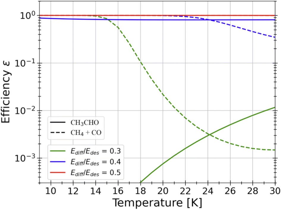 | ||
| Fig. 11 QM computations of the efficiency of the reaction CH3 + HCO leading to either CH3CHO (solid lines) or CO + CH4 (dashed lines) as a function of the temperature of the water ice.168 Three different values for Edif/BE ratios were considered in these computations: 0.3 (green), 0.4 (blue) and 0.5 (red). Depending on this value, which is practically unknown, acetaldehyde could easily form on the icy surfaces or not form at all. | ||
Finally, it is important to emphasize that, in practice, each case is peculiar and requires a dedicated study. At present about two dozen systems have been studied on the water surfaces186 and much less on CO-rich ices.187
Only one public database exists so far with a list of grain-surface reactions, posted on the KIDA website. The list is based on Garrod and collaborators’ reaction network129,183 and it is presented in a work by Ruaud and collaborators.130
5 Formation of iCOMs: observations against predictions
In this last part, I will discuss a few specific cases, trying to provide ideas rather than a precise comparison with specific models, which – as I hope I convince the reader – depend on many processes and quantities on which we do not have a full control, in my opinion.5.1 Ethanol, glycolaldehyde and acetaldehyde
Observations towards warm objects (hot cores, hot corinos and molecular shocks) show that there exists a correlation between the measured ethanol and glycolaldehyde abundances.36,188,189 In addition, the measured abundance of glycolaldehyde also correlates with acetaldehyde, as shown in Fig. 12. A simple explanation, very often assumed by several authors, is that the three species are all grain-surface chemistry products, basically following the scheme “Only grain chemistry” described in Section 4.2.5. Often, the combination of CH3 and HCO radicals are invoked for acetaldehyde formation, but as discussed in Section 4.2.5 is far from the consolidated route of acetaldehyde formation.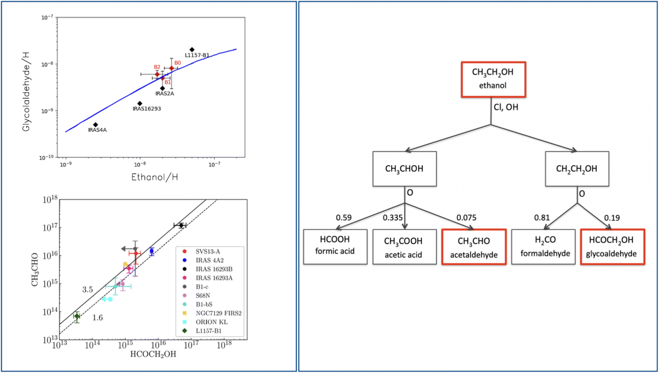 | ||
| Fig. 12 Gas-phase formation route of glycolaldehyde and acetaldehyde from ethanol. Left panel: observed correlations between the measured abundances of glycolaldehyde and ethanol (upper panel)160 and column densities of acetaldehyde and glycolaldehyde (bottom panel).158 The upper panel shows the value derived for the shocked region L1157-B1: the black diamonds show the values obtained with the single-dish IRAM-30m observations188 while the red diamonds show the values obtained in the three blobs in which the B1 region splits when observed with the interferometer NOEMA (Robuschi et al. in prep). Right panel: the proposed gas-phase chain of reactions that form acetaldehyde and glycolaldehyde starting from ethanol,160 which would be the grain-surface product.124 | ||
However, there is also the possibility that the three species are chemically linked and not all of them are a grain-surface chemistry product. Skouteris, Balucani and collaborators proposed that glycolaldehyde is actually a gas-phase product, a daughter of ethanol, following the chain of reactions shown in Fig. 12 (right panel). The same chain of reactions would also form acetaldehyde. Following up on the possibility that ethanol, now perhaps observed in the solid form by JWST, is synthesised on the grain surfaces by the CCH + H2O reaction (followed by an H addition),124 glycolaldehyde and acetaldehyde could be siblings and both gas-phase products. The QM computations of the branching ratios rate coefficients of the glycolaldehyde formation would produce model predictions that fit very well with the observations (Fig. 12 (ref. 160)). In the same vein, the acetaldehyde over glycolaldehyde abundance ratio predicted by the QM computations branching ratios fit very well with the observed one (Fig. 12 (ref. 158)).
In addition, the measured deuteration of glycolaldehyde and acetaldehyde, and their isomers, are also in good agreement with those predicted by QM computations.158,190 Unfortunately, no predictions of the deuteration for these two molecules exist in the literature. Therefore, while the gas-phase origin hypothesis has passed the possible tests so far available, the grain-surface one can not be excluded for lack of similar precise predictions from QM computations.
5.2 Formamide
This has been one of the most debated cases in the context of iCOM formation (see, for example, the exhaustive review by López-Sepulcre and collaborators191). In 2013, Kahane and collaborators suggested the possibility that NH2CHO is formed in the gas-phase via the reaction of NH2 with formaldehyde.192 Two years later, Barone and collaborators presented QM computations showing that the reaction has an embedded barrier.193 However, later QM computations by Song and Kästner194 argued that the barrier is actually larger than that predicted by Barone et al. and that, consequently, the reaction is inefficient at the ISM temperatures. The height of the barrier was successively revised by Skouteris, Vazart and collaborators, who found a larger value than that of Barone et al., but one still small enough for the reaction to be fast in warm gas (∼100 K).195,196 Specifically, Skouteris et al. predicted a rate constant at 100 K equal to 1.2 × 10⁻¹³ cm3 s−1 and, using this value, were capable of reproducing the observations of formamide towards L1157-B1, as reported in Section 3.3.Yet, the saga did not stop here. A recent experiment on the NH2 + H2CO reaction carried out by Douglas, Heard and collaborators at 34 K with a CRESU apparatus, failed to detect formamide.197 These authors put an upper limit on the rate constant equal to 6 × 10⁻¹² cm3 s−1, namely 2.5 times larger than the predicted one by Skouteris et al. at the same temperature. Douglas et al. complemented the experimental results with new QM computations, whose accuracy is essentially the same as of those by Song and Kästner,194 and insisted on the presence of an non-embedded activation barrier, which would lead to a much lower rate constant at temperatures ≤200 K.
The presence/absence of the barrier is linked to how the pre-reactant complex (PRC) is computationally treated and whether the zero-point-energy (ZPE) should be added or not to the transition state (TS) towards the formation of formamide. Barone, Skouteris and collaborators193,195,196 claimed that the ZPE, computed with the standard methods adopted by the other authors,194,197 should not be added to the PRC TS energy because the PRC has very loose modes which would not substantially alter the TS energy height. In contrast, Song, Kästner, Douglas, Heard and collaborators194,197 think the opposite and they consider the ZPE of the PRC computed in the harmonic approximation. Since the various approximations used for the computations of the standard TS very likely do not apply to the PRC, at this stage, it is impossible to affirm with certainty who is right and whether the ZPE of the PRC may lead to an activation barrier for the H2CO + NH2. New calculations with more adapted methods should be employed, or a lower upper limit in experimental works should be obtained. In summary, unfortunately the new experimental work by Douglas et al.197 does not bring new meaningful constraints when compared to the QM predictions of Barone, Skouteris and collaborators.
Astronomical observations could be used to distinguish whether the dominant route of formation of formamide is the gas-phase or grain-surface. The analysis of the displacement of acetaldehyde and formamide in L1157-B1, shown in Fig. 6, would be in favor of the gas-phase route for formamide.44 In addition, as for glycolaldehyde and acetaldehyde, it is possible to compare the theoretical predictions, based on QM computations of the gas-phase reaction NH2 + H2CO, on the deuteration of formamide and its isomers,196 with the observations towards the IRAS16293-2422 A2 hot corino observed by the PILS team.67 In this case, the predictions agree extremely well with the observed values. As for the case of glycolaldehyde and acetaldehyde, the compatibility of the predicted abundances obtained assuming the gas-phase reaction route with the observations available in the literature, are necessary but insufficient.
The formamide formation on the grain surfaces has also been a saga. The observed correlation between the abundance of formamide with that of HCNO was immediately seen as proof that NH2HCO is the result of HNCO hydrogenation.198,199 This hypothesis was ruled out by the experiment by Noble, Theule and collaborators.200 Successive similar experiments showed that there is indeed recycling between NH2HCO and HNCO, with the H atom acquired and lost on each side, with a result in favor of H abstraction from NH2HCO (and not the other way around).201 Other possibilities evoked in the literature consider the NH2 + HCO recombination on the grain surfaces129 and the formation from the CN landing on the ice surface and reacting with a water molecule.164
6 Conclusions
The progress in astrochemistry and, in particular, the study of the formation of interstellar complex organic molecules (iCOMs) has proceeded at a vertiginous speed on all fronts: observations, laboratory experiments, quantum mechanics computations and modeling. It is difficult to consider everything and cite everybody in a review of a few pages, I did my best but I am conscious that my opinions enter in my writing. That said, I hope that this review provides a correct view of the passionate and fascinating discussions around the subject, as well as the many limits to our knowledge.Progress towards a final theory on how iCOMs form and thrive during the formation of a planetary system similar to our solar system can only come from a very tight collaboration between astronomers and chemists. This is not only a curiosity, it may also be key for progressing our knowledge of the emergence of life on Earth, and maybe in other systems. After all, when one considers the major ingredients (elements) necessary for terrestrial life, they are an exact match of the most abundant elements at the moment our solar system formed: hydrogen, oxygen, carbon, nitrogen, sulphur and so on, literally reflecting the sequence of initial elemental abundances of the solar nebula. It may be a cause or a consequence: yet, life used what was available, in terms of elements. Notice, however, that once the Earth formed, the abundance of elements around for life to start was completely changed, with the most abundant ones no longer being hydrogen, oxygen, carbon and so on. It seems to me that life likely bears the chemical imprint of the first phases of solar system formation.
Finally, no doubt life used the laws that regulate the Universe, namely the physics and chemistry that we know. Whether the iCOMs formed during the infancy of the solar system had a role or not, this first chapter of our history has to be written in as much detail as possible.
Conflicts of interest
There are no conflicts to declare.Acknowledgements
I would like to warmly thank my chemist friends and collaborators Nadia Balucani, Piero Ugliengo, Albert Rimola: without their help and teaching, this review would not have existed. I also thank my astronomer friends and collaborators, especially Claudio Codella, Ana López-Sepulcre, Charlotte Vastel and Bertrand Lefloch. A final very deep thank goes to the young researchers with whom I had the luck to work, especially Eleonora Bianchi, Mathilde Bouvier, Marta De Simone, Joan Enrique-Romero, Cecile Favre, Lorenzo Tinacci and Fanny Vazart. I acknowledge the funding within the European Union’s Horizon 2020 research and innovation programme from the European Research Council (ERC) for the project “The Dawn of Organic Chemistry” (DOC), grant agreement No. 741002, and from the Marie Sklodowska-Curie for the project “Astro-Chemical Origins” (ACO), grant agreement No. 811312.Notes and references
- J. K. Jørgensen, T. L. Bourke, P. C. Myers, J. Di Francesco, E. F. van Dishoeck, C.-F. Lee, N. Ohashi, F. L. Schöier, S. Takakuwa, D. J. Wilner and Q. Zhang, Astrophys. J., 2007, 659, 479–498 CrossRef.
- V. Taquet, A. López-Sepulcre, C. Ceccarelli, R. Neri, C. Kahane and S. B. Charnley, Astrophys. J., 2015, 804, 81 CrossRef.
- M. De Simone, C. Ceccarelli, C. Codella, B. E. Svoboda, C. Chandler, M. Bouvier, S. Yamamoto, N. Sakai, P. Caselli, C. Favre, L. Loinard, B. Lefloch, H. B. Liu, A. López-Sepulcre, J. E. Pineda, V. Taquet and L. Testi, Astrophys. J., 2020, 896, L3 CrossRef CAS.
- A. López-Sepulcre, N. Sakai, R. Neri, M. Imai, Y. Oya, C. Ceccarelli, A. E. Higuchi, Y. Aikawa, S. Bottinelli, E. Caux, T. Hirota, C. Kahane, B. Lefloch, C. Vastel, Y. Watanabe and S. Yamamoto, Astron. Astrophys., 2017, 606, A121 CrossRef.
- C. Ceccarelli, P. Caselli, F. Fontani, R. Neri, A. López-Sepulcre, C. Codella, S. Feng, I. Jiménez-Serra, B. Lefloch, J. E. Pineda, C. Vastel, F. Alves, R. Bachiller, N. Balucani, E. Bianchi, L. Bizzocchi, S. Bottinelli, E. Caux, A. Chacón-Tanarro, R. Choudhury, A. Coutens, F. Dulieu, C. Favre, P. Hily-Blant, J. Holdship, C. Kahane, A. Jaber Al-Edhari, J. Laas, J. Ospina, Y. Oya, L. Podio, A. Pon, A. Punanova, D. Quenard, A. Rimola, N. Sakai, I. R. Sims, S. Spezzano, V. Taquet, L. Testi, P. Theulé, P. Ugliengo, A. I. Vasyunin, S. Viti, L. Wiesenfeld and S. Yamamoto, Astrophys. J., 2017, 850, 176 CrossRef.
- E. Herbst and E. F. van Dishoeck, Annu. Rev. Astron. Astrophys., 2009, 47, 427–480 CrossRef CAS.
- P. Caselli and C. Ceccarelli, Astron. Astrophys. Rev., 2012, 20, 56 CrossRef.
- C. Ceccarelli, P. Caselli, D. Bockelée-Morvan, O. Mousis, S. Pizzarello, F. Robert and D. Semenov, Protostars and Planets VI, 2014, pp. 859–882 Search PubMed.
- K. I. Öberg, Chem. Rev., 2016, 116, 9631 CrossRef PubMed.
- J. K. Jørgensen, A. Belloche and R. T. Garrod, Annu. Rev. Astron. Astrophys., 2020, 58, 727–778 CrossRef.
- K. I. Öberg and E. A. Bergin, Phys. Rep., 2021, 893, 1–48 CrossRef.
- C. Ceccarelli, C. Codella, N. Balucani, D. Bockelée-Morvan, E. Herbst, C. Vastel, P. Caselli, C. Favre, B. Lefloch and K. Öberg, arXiv, 2022, preprint, arXiv:2206.13270.
- A. Morbidelli, J. Chambers, J. I. Lunine, J. M. Petit, F. Robert, G. B. Valsecchi and K. E. Cyr, Elements, 2022, 18, 155 CrossRef.
- L. Piani, Y. Marrocchi, T. Rigaudier, L. G. Vacher, D. Thomassin and B. Marty, Science, 2020, 369, 1110–1113 CrossRef CAS PubMed.
- C. Ceccarelli and F. Du, Elements, 2022, 18, 155 CrossRef CAS.
- F. Ober, S. Wolf, A. L. Uribe and H. H. Klahr, Astron. Astrophys., 2015, 579, A105 CrossRef.
- P. Mollière, T. Molyarova, B. Bitsch, T. Henning, A. Schneider, L. Kreidberg, C. Eistrup, R. Burn, E. Nasedkin, D. Semenov, C. Mordasini, M. Schlecker, K. R. Schwarz, S. Lacour, M. Nowak and M. Schulik, Astrophys. J., 2022, 934, 74 CrossRef.
- J. L. Linsky, B. T. Draine, H. W. Moos, E. B. Jenkins, B. E. Wood, C. Oliveira, W. P. Blair, S. D. Friedman, C. Gry, D. Knauth, J. W. Kruk, S. Lacour, N. Lehner, S. Redfield, J. M. Shull, G. Sonneborn and G. M. Williger, Astrophys. J., 2006, 647, 1106–1124 CrossRef CAS.
- A. Bacmann, B. Lefloch, C. Ceccarelli, J. Steinacker, A. Castets and L. Loinard, Astrophys. J., 2003, 585, L55–L58 CrossRef CAS.
- A. Bacmann, V. Taquet, A. Faure, C. Kahane and C. Ceccarelli, Astron. Astrophys., 2012, 541, L12 CrossRef.
- J. Cernicharo, N. Marcelino, E. Roueff, M. Gerin, A. Jiménez-Escobar and G. M. Muñoz Caro, Astrophys. J., 2012, 759, L43 CrossRef.
- K. I. Öberg, S. Bottinelli, J. K. Jørgensen and E. F. van Dishoeck, Astrophys. J., 2010, 716, 825–834 CrossRef.
- A. A. Jaber, C. Ceccarelli, C. Kahane and E. Caux, Astrophys. J., 2014, 791, 29 CrossRef.
- C. Vastel, C. Ceccarelli, B. Lefloch and R. Bachiller, Astrophys. J., 2014, 795, L2 CrossRef.
- L. Bizzocchi, P. Caselli, S. Spezzano and E. Leonardo, Astron. Astrophys., 2014, 569, A27 CrossRef.
- I. Jiménez-Serra, A. I. Vasyunin, P. Caselli, N. Marcelino, N. Billot, S. Viti, L. Testi, C. Vastel, B. Lefloch and R. Bachiller, Astrophys. J., 2016, 830, L6 CrossRef.
- C. Vastel, J. C. Loison, V. Wakelam and B. Lefloch, Astron. Astrophys., 2019, 625, A91 CrossRef CAS.
- S. Scibelli and Y. Shirley, Astrophys. J., 2020, 891, 73 CrossRef CAS.
- S. Spezzano, L. Bizzocchi, P. Caselli, J. Harju and S. Brünken, Astron. Astrophys., 2016, 592, L11 CrossRef.
- C. Zhou, C. Vastel, J. Montillaud, C. Ceccarelli, K. Demyk, J. Harju, M. Juvela, I. Ristorcelli and T. Liu, Astron.Astrophys., 2022, 658, A131 CrossRef CAS.
- M. Imai, N. Sakai, Y. Oya, A. López-Sepulcre, Y. Watanabe, C. Ceccarelli, B. Lefloch, E. Caux, C. Vastel, C. Kahane, T. Sakai, T. Hirota, Y. Aikawa and S. Yamamoto, Astrophys. J., 2016, 830, L37 CrossRef.
- S. Cazaux, A. G. G. M. Tielens, C. Ceccarelli, A. Castets, V. Wakelam, E. Caux, B. Parise and D. Teyssier, Astrophys. J., 2003, 593, L51–L55 CrossRef CAS.
- S. Bottinelli, C. Ceccarelli, R. Neri, J. P. Williams, E. Caux, S. Cazaux, B. Lefloch, S. Maret and A. G. G. M. Tielens, Astrophys. J., 2004, 617, L69–L72 CrossRef CAS.
- Y.-J. Kuan, H.-C. Huang, S. B. Charnley, N. Hirano, S. Takakuwa, D. J. Wilner, S.-Y. Liu, N. Ohashi, T. L. Bourke, C. Qi and Q. Zhang, Astrophys. J., 2004, 616, L27–L30 CrossRef CAS.
- E. Bianchi, C. J. Chandler, C. Ceccarelli, C. Codella, N. Sakai, A. López-Sepulcre, L. T. Maud, G. Moellenbrock, B. Svoboda, Y. Watanabe, T. Sakai, F. Ménard, Y. Aikawa, F. Alves, N. Balucani, M. Bouvier, P. Caselli, E. Caux, S. Charnley, S. Choudhury, M. De Simone, F. Dulieu, A. Durán, L. Evans, C. Favre, D. Fedele, S. Feng, F. Fontani, L. Francis, T. Hama, T. Hanawa, E. Herbst, T. Hirota, M. Imai, A. Isella, I. Jiménez-Serra, D. Johnstone, C. Kahane, B. Lefloch, L. Loinard, M. J. Maureira, S. Mercimek, A. Miotello, S. Mori, R. Nakatani, H. Nomura, Y. Oba, S. Ohashi, Y. Okoda, J. Ospina-Zamudio, Y. Oya, J. Pineda, L. Podio, A. Rimola, D. S. Cox, Y. Shirley, V. Taquet, L. Testi, C. Vastel, S. Viti, N. Watanabe, A. Witzel, C. Xue, Y. Zhang, B. Zhao and S. Yamamoto, Mon. Not. R. Astron. Soc.: Lett., 2020, 498, L87–L92 CrossRef CAS.
- Y.-L. Yang, N. Sakai, Y. Zhang, N. M. Murillo, Z. E. Zhang, A. E. Higuchi, S. Zeng, A. López-Sepulcre, S. Yamamoto, B. Lefloch, M. Bouvier, C. Ceccarelli, T. Hirota, M. Imai, Y. Oya, T. Sakai and Y. Watanabe, Astrophys. J., 2021, 910, 20 CrossRef CAS.
- Y. Oya, N. Sakai, Y. Watanabe, A. E. Higuchi, T. Hirota, A. López-Sepulcre, T. Sakai, Y. Aikawa, C. Ceccarelli, B. Lefloch, E. Caux, C. Vastel, C. Kahane and S. Yamamoto, Astrophys. J., 2017, 837, 174 CrossRef.
- N. Marcelino, M. Gerin, J. Cernicharo, A. Fuente, H. A. Wootten, E. Chapillon, J. Pety, D. C. Lis, E. Roueff, B. Commerçon and A. Ciardi, Astron. Astrophys., 2018, 620, A80 CrossRef CAS PubMed.
- K. I. Öberg, T. Lauck and D. Graninger, Astrophys. J., 2014, 788, 68 CrossRef.
- S. Bottinelli, C. Ceccarelli, B. Lefloch, J. P. Williams, A. Castets, E. Caux, S. Cazaux, S. Maret, B. Parise and A. G. G. M. Tielens, Astrophys. J., 2004, 615, 354–358 CrossRef CAS.
- S. Bottinelli, C. Ceccarelli, J. P. Williams and B. Lefloch, Astron. Astrophys., 2007, 463, 601–610 CrossRef CAS.
- E. Bianchi, C. Codella, C. Ceccarelli, F. Vazart, R. Bachiller, N. Balucani, M. Bouvier, M. De Simone, J. Enrique-Romero, C. Kahane, B. Lefloch, A. López-Sepulcre, J. Ospina-Zamudio, L. Podio and V. Taquet, Mon. Not. R. Astron. Soc., 2019, 483, 1850–1861 CrossRef CAS.
- E. Bianchi, C. Ceccarelli, C. Codella, A. López-Sepulcre, S. Yamamoto, N. Balucani, P. Caselli, L. Podio, R. Neri, R. Bachiller, C. Favre, F. Fontani, B. Lefloch, N. Sakai and D. Segura-Cox, Astron. Astrophys., 2022, 662, A103 CrossRef CAS.
- C. Codella, C. Ceccarelli, P. Caselli, N. Balucani, V. Barone, F. Fontani, B. Lefloch, L. Podio, S. Viti, S. Feng, R. Bachiller, E. Bianchi, F. Dulieu, I. Jiménez-Serra, J. Holdship, R. Neri, J. E. Pineda, A. Pon, I. Sims, S. Spezzano, A. I. Vasyunin, F. Alves, L. Bizzocchi, S. Bottinelli, E. Caux, A. Chacón-Tanarro, R. Choudhury, A. Coutens, C. Favre, P. Hily-Blant, C. Kahane, A. Jaber Al-Edhari, J. Laas, A. López-Sepulcre, J. Ospina, Y. Oya, A. Punanova, C. Puzzarini, D. Quenard, A. Rimola, N. Sakai, D. Skouteris, V. Taquet, L. Testi, P. Theulé, P. Ugliengo, C. Vastel, F. Vazart, L. Wiesenfeld and S. Yamamoto, Astron. Astrophys., 2017, 605, L3 CrossRef.
- C.-F. Lee, Z.-Y. Li, P. T. P. Ho, N. Hirano, Q. Zhang and H. Shang, Astrophys. J., 2017, 843, 27 CrossRef.
- L. Chahine, A. López-Sepulcre, R. Neri, C. Ceccarelli, S. Mercimek, C. Codella, M. Bouvier, E. Bianchi, C. Favre, L. Podio, F. O. Alves, N. Sakai and S. Yamamoto, Astron. Astrophys., 2022, 657, A78 CrossRef CAS.
- S.-Y. Hsu, S.-Y. Liu, T. Liu, D. Sahu, N. Hirano, C.-F. Lee, K. Tatematsu, G. Kim, M. Juvela, P. Sanhueza, J. He, D. Johnstone, S.-L. Qin, L. Bronfman, H.-R. V. Chen, S. Dutta, D. J. Eden, K.-S. Jhan, K.-T. Kim, Y.-J. Kuan, W. Kwon, C. W. Lee, J.-E. Lee, A. Moraghan, M. G. Rawlings, H. Shang, A. Soam, M. A. Thompson, A. Traficante, Y. Wu, Y.-L. Yang and Q. Zhang, Astrophys. J., 2020, 898, 107 CrossRef CAS.
- M. Bouvier, C. Ceccarelli, A. López-Sepulcre, N. Sakai, S. Yamamoto and Y.-L. Yang, Astrophys. J., 2022, 929, 10 CrossRef.
- R. Martín-Doménech, J. B. Bergner, K. I. Öberg and J. K. Jørgensen, Astrophys. J., 2019, 880, 130 CrossRef.
- J. B. Bergner, R. Martín-Doménech, K. I. Öberg, J. K. Jørgensen, E. Artur de la Villarmois and C. Brinch, ACS Earth Space Chem., 2019, 3, 1564–1575 CrossRef CAS.
- G. Molpeceres, J. Kästner, V. J. Herrero, R. J. Peláez and B. Maté, Astron. Astrophys., 2022, 664, A169 CrossRef CAS.
- R. H. Rubin, G. W. Swenson Jr, R. C. Benson, H. L. Tigelaar and W. H. Flygare, Astrophys. J., 1971, 169, L39 CrossRef CAS.
- G. A. Blake, E. C. Sutton, C. R. Masson and T. G. Phillips, Astrophys. J., 1987, 315, 621 CrossRef CAS.
- C. Ceccarelli, L. Loinard, A. Castets, A. Faure and B. Lefloch, Astron. Astrophys., 2000, 362, 1122–1126 CAS.
- C. Ceccarelli, P. Caselli, E. Herbst, A. G. G. M. Tielens and E. Caux, Protostars and Planets V, 2007, pp. 47–62 Search PubMed.
- A. Belloche, A. J. Maury, S. Maret, S. Anderl, A. Bacmann, P. André, S. Bontemps, S. Cabrit, C. Codella, M. Gaudel, F. Gueth, C. Lefèvre, B. Lefloch, L. Podio and L. Testi, Astron. Astrophys., 2020, 635, A198 CrossRef CAS.
- C. Ceccarelli, L. Loinard, A. Castets, A. G. G. M. Tielens and E. Caux, Astron. Astrophys., 2000, 357, L9–L12 CAS.
- J. K. Jørgensen, C. Favre, S. E. Bisschop, T. L. Bourke, E. F. van Dishoeck and M. Schmalzl, Astrophys. J., 2012, 757, L4 CrossRef.
- J. K. Jørgensen, M. H. D. van der Wiel, A. Coutens, J. M. Lykke, H. S. P. Müller, E. F. van Dishoeck, H. Calcutt, P. Bjerkeli, T. L. Bourke, M. N. Drozdovskaya, C. Favre, E. C. Fayolle, R. T. Garrod, S. K. Jacobsen, K. I. Öberg, M. V. Persson and S. F. Wampfler, Astron. Astrophys., 2016, 595, A117 CrossRef.
- S. Manigand, J. K. Jørgensen, H. Calcutt, H. S. P. Müller, N. F. W. Ligterink, A. Coutens, M. N. Drozdovskaya, E. F. van Dishoeck and S. F. Wampfler, Astron. Astrophys., 2020, 635, A48 CrossRef CAS.
- S. Manigand, A. Coutens, J. C. Loison, V. Wakelam, H. Calcutt, H. S. P. Müller, J. K. Jørgensen, V. Taquet, S. F. Wampfler, T. L. Bourke, B. M. Kulterer, E. F. van Dishoeck, M. N. Drozdovskaya and N. F. W. Ligterink, Astron. Astrophys., 2021, 645, A53 CrossRef CAS.
- E. Bianchi, A. López-Sepulcre, C. Ceccarelli, C. Codella, L. Podio, M. Bouvier and J. Enrique-Romero, Astrophys. J., 2022, 928, L3 CrossRef.
- C. Ceccarelli, A. Castets, L. Loinard, E. Caux and A. G. G. M. Tielens, Astron. Astrophys., 1998, 338, L43–L46 CAS.
- B. Parise, C. Ceccarelli, A. G. G. M. Tielens, A. Castets, E. Caux, B. Lefloch and S. Maret, Astron. Astrophys., 2006, 453, 949–958 CrossRef CAS.
- B. Parise, A. Castets, E. Herbst, E. Caux, C. Ceccarelli, I. Mukhopadhyay and A. G. G. M. Tielens, Astron. Astrophys., 2004, 416, 159–163 CrossRef CAS.
- C. Richard, L. Margulès, E. Caux, C. Kahane, C. Ceccarelli, J. C. Guillemin, R. A. Motiyenko, C. Vastel and P. Groner, Astron. Astrophys., 2013, 552, A117 CrossRef.
- A. Coutens, J. K. Jørgensen, M. H. D. van der Wiel, H. S. P. Müller, J. M. Lykke, P. Bjerkeli, T. L. Bourke, H. Calcutt, M. N. Drozdovskaya, C. Favre, E. C. Fayolle, R. T. Garrod, S. K. Jacobsen, N. F. W. Ligterink, K. I. Öberg, M. V. Persson, E. F. van Dishoeck and S. F. Wampfler, Astron. Astrophys., 2016, 590, L6 CrossRef.
- J. K. Jørgensen, H. S. P. Müller, H. Calcutt, A. Coutens, M. N. Drozdovskaya, K. I. Öberg, M. V. Persson, V. Taquet, E. F. van Dishoeck and S. F. Wampfler, Astron. Astrophys., 2018, 620, A170 CrossRef.
- M. V. Persson, J. K. Jørgensen, H. S. P. Müller, A. Coutens, E. F. van Dishoeck, V. Taquet, H. Calcutt, M. H. D. van der Wiel, T. L. Bourke and S. F. Wampfler, Astron. Astrophys., 2018, 610, A54 CrossRef.
- S. Manigand, H. Calcutt, J. K. Jørgensen, V. Taquet, H. S. P. Müller, A. Coutens, S. F. Wampfler, N. F. W. Ligterink, M. N. Drozdovskaya, L. E. Kristensen, M. H. D. van der Wiel and T. L. Bourke, Astron. Astrophys., 2019, 623, A69 CrossRef CAS.
- C. Richard, J. K. Jørgensen, L. Margulès, R. A. Motiyenko, J. C. Guillemin and P. Groner, Astron. Astrophys., 2021, 651, A120 CrossRef CAS.
- M. De Simone, C. Ceccarelli, C. Codella, B. E. Svoboda, C. J. Chandler, M. Bouvier, S. Yamamoto, N. Sakai, Y.-L. Yang, P. Caselli, B. Lefloch, H. B. Liu, A. López-Sepulcre, L. Loinard, J. E. Pineda and L. Testi, Astrophys. J., 2022, 935, L14 CrossRef.
- R. Bachiller, S. Liechti, C. M. Walmsley and F. Colomer, Astron. Astrophys., 1995, 295, L51 CAS.
- R. Bachiller and M. Pérez Gutiérrez, Astrophys. J., 1997, 487, L93–L96 CrossRef CAS.
- C. Vastel, F. Alves, C. Ceccarelli, M. Bouvier, I. Jiménez-Serra, T. Sakai, P. Caselli, L. Evans, F. Fontani, R. Le Gal, C. J. Chandler, B. Svoboda, L. Maud, C. Codella, N. Sakai, A. López-Sepulcre, G. Moellenbrock, Y. Aikawa, N. Balucani, E. Bianchi, G. Busquet, E. Caux, S. Charnley, N. Cuello, M. De Simone, F. Dulieu, A. Durân, D. Fedele, S. Feng, L. Francis, T. Hama, T. Hanawa, E. Herbst, T. Hirota, M. Imai, A. Isella, D. Johnstone, B. Lefloch, L. Loinard, M. Maureira, N. M. Murillo, S. Mercimek, S. Mori, F. Menard, A. Miotello, R. Nakatani, H. Nomura, Y. Oba, S. Ohashi, Y. Okoda, J. Ospina-Zamudio, Y. Oya, J. E. Pineda, L. Podio, A. Rimola, D. Segura Cox, Y. Shirley, L. Testi, S. Viti, N. Watanabe, Y. Watanabe, A. Witzel, C. Xue, Y. Zhang, B. Zhao and S. Yamamoto, Astron. Astrophys., 2022, 664, A171 CrossRef CAS.
- F. Gueth, S. Guilloteau and R. Bachiller, Astron. Astrophys., 1996, 307, 891–897 CAS.
- F. Fontani, C. Codella, C. Ceccarelli, B. Lefloch, S. Viti and M. Benedettini, Astrophys. J., 2014, 788, L43 CrossRef.
- K. I. Öberg, V. V. Guzmán, K. Furuya, C. Qi, Y. Aikawa, S. M. Andrews, R. Loomis and D. J. Wilner, Nature, 2015, 520, 198–201 CrossRef PubMed.
- C. Favre, D. Fedele, D. Semenov, S. Parfenov, C. Codella, C. Ceccarelli, E. A. Bergin, E. Chapillon, L. Testi, F. Hersant, B. Lefloch, F. Fontani, G. A. Blake, L. I. Cleeves, C. Qi, K. R. Schwarz and V. Taquet, Astrophys. J., 2018, 862, L2 CrossRef.
- K. I. Öberg, V. V. Guzmán, C. Walsh, Y. Aikawa, E. A. Bergin, C. J. Law, R. A. Loomis, F. Alarcón, S. M. Andrews, J. Bae, J. B. Bergner, Y. Boehler, A. S. Booth, A. D. Bosman, J. K. Calahan, G. Cataldi, L. I. Cleeves, I. Czekala, K. Furuya, J. Huang, J. D. Ilee, N. T. Kurtovic, R. Le Gal, Y. Liu, F. Long, F. Ménard, H. Nomura, L. M. Pérez, C. Qi, K. R. Schwarz, A. Sierra, R. Teague, T. Tsukagoshi, Y. Yamato, M. L. R. van’t Hoff, A. R. Waggoner, D. J. Wilner and K. Zhang, Astrophys. J. Suppl., 2021, 257, 1 CrossRef.
- J. D. Ilee, C. Walsh, A. S. Booth, Y. Aikawa, S. M. Andrews, J. Bae, E. A. Bergin, J. B. Bergner, A. D. Bosman, G. Cataldi, L. I. Cleeves, I. Czekala, V. V. Guzmán, J. Huang, C. J. Law, R. Le Gal, R. A. Loomis, F. Ménard, H. Nomura, K. I. Öberg, C. Qi, K. R. Schwarz, R. Teague, T. Tsukagoshi, D. J. Wilner, Y. Yamato and K. Zhang, Astrophys. J. Suppl., 2021, 257, 9 CrossRef CAS.
- C. Walsh, R. A. Loomis, K. I. Öberg, M. Kama, M. L. R. van’t Hoff, T. J. Millar, Y. Aikawa, E. Herbst, S. L. Widicus Weaver and H. Nomura, Astrophys. J., 2016, 823, L10 CrossRef.
- P. Nazari, B. Tabone, G. P. Rosotti, M. L. van Gelder, R. Meshaka and E. F. van Dishoeck, Astron. Astrophys., 2022, 663, A58 CrossRef CAS.
- L. Podio, A. Garufi, C. Codella, D. Fedele, E. Bianchi, F. Bacciotti, C. Ceccarelli, C. Favre, S. Mercimek, K. Rygl and L. Testi, Astron. Astrophys., 2020, 642, L7 CrossRef CAS.
- L. Keyte, M. Kama, A. S. Booth, E. A. Bergin, L. I. Cleeves, E. F. van Dishoeck, M. N. Drozdovskaya, K. Furuya, J. Rawlings, O. Shorttle and C. Walsh, Nat. Astron., 2023, 7, 684 CrossRef.
- S. L. Grant, E. F. van Dishoeck, B. Tabone, D. Gasman, T. Henning, I. Kamp, M. Güdel, P.-O. Lagage, G. Bettoni, G. Perotti, V. Christiaens, M. Samland, A. M. Arabhavi, I. Argyriou, A. Abergel, O. Absil, D. Barrado, A. Boccaletti, J. Bouwman, A. C. o. Garatti, V. Geers, A. M. Glauser, R. Guadarrama, H. Jang, J. Kanwar, F. Lahuis, M. Morales-Calderón, M. Mueller, C. Nehmé, G. Olofsson, E. Pantin, N. Pawellek, T. P. Ray, D. Rodgers-Lee, S. Scheithauer, J. Schreiber, K. Schwarz, M. Temmink, B. Vandenbussche, M. Vlasblom, L. B. F. M. Waters, G. Wright, L. Colina, T. R. Greve, K. Justannont and G. Östlin, Astrophys. J., 2023, 947, L6 CrossRef.
- A. Banzatti, K. M. Pontoppidan, J. Pére Chávez, C. Salyk, L. Diehl, S. Bruderer, G. J. Herczeg, A. Carmona, I. Pascucci, S. Brittain, S. Jensen, S. Grant, E. F. van Dishoeck, I. Kamp, A. D. Bosman, K. I. Öberg, G. A. Blake, M. R. Meyer, E. Gaidos, A. Boogert, J. T. Rayner and C. Wheeler, Astron. J., 2023, 165, 72 CrossRef.
- C.-F. Lee, P. T. P. Ho, Z.-Y. Li, N. Hirano, Q. Zhang and H. Shang, Nat. Astron., 2017, 1, 0152 CrossRef.
- C. Codella, E. Bianchi, B. Tabone, C. F. Lee, S. Cabrit, C. Ceccarelli, L. Podio, F. Bacciotti, R. Bachiller, E. Chapillon, F. Gueth, A. Gusdorf, B. Lefloch, S. Leurini, G. Pineau des Forêts, K. L. J. Rygl and M. Tafalla, Astron. Astrophys., 2018, 617, A10 CrossRef.
- C.-F. Lee, C. Codella, Z.-Y. Li and S.-Y. Liu, Astrophys. J., 2019, 876, 63 CrossRef CAS.
- C.-F. Lee, C. Codella, C. Ceccarelli and A. López-Sepulcre, Astrophys. J., 2022, 937, 10 CrossRef.
- E. C. Pickering, Astron. Nachr., 1890, 124, 113 CrossRef.
- M. S. Connelley and B. Reipurth, Astrophys. J., 2018, 861, 145 CrossRef.
- K. M. Strom and S. E. Strom, Astrophys. J., 1993, 412, L63 CrossRef CAS.
- E. Furlan, W. J. Fischer, B. Ali, A. M. Stutz, T. Stanke, J. J. Tobin, S. T. Megeath, M. Osorio, L. Hartmann, N. Calvet, C. A. Poteet, J. Booker, P. Manoj, D. M. Watson and L. Allen, Astrophys. J., Suppl. Ser., 2016, 224, 5 CrossRef.
- W. J. Fischer, E. Safron and S. T. Megeath, American Astronomical Society Meeting Abstracts #228, 2016, p. 308.01 Search PubMed.
- L. A. Cieza, S. Casassus, J. Tobin, S. P. Bos, J. P. Williams, S. Perez, Z. Zhu, C. Caceres, H. Canovas, M. M. Dunham, A. Hales, J. L. Prieto, D. A. Principe, M. R. Schreiber, D. Ruiz-Rodriguez and A. Zurlo, Nature, 2016, 535, 258–261 CrossRef CAS PubMed.
- M. L. R. van’t Hoff, J. J. Tobin, L. Trapman, D. Harsono, P. D. Sheehan, W. J. Fischer, S. T. Megeath and E. F. van Dishoeck, Astrophys. J., 2018, 864, L23 CrossRef.
- J.-E. Lee, S. Lee, G. Baek, Y. Aikawa, L. Cieza, S.-Y. Yoon, G. Herczeg, D. Johnstone and S. Casassus, Nat. Astron., 2019, 3, 314–319 CrossRef.
- M. Leemker, M. L. R. van’t Hoff, L. Trapman, M. L. van Gelder, M. R. Hogerheijde, D. Ruíz-Rodríguez and E. F. van Dishoeck, Astron. Astrophys., 2021, 646, A3 CrossRef CAS.
- J. J. Tobin, M. L. R. van’t Hoff, M. Leemker, E. F. van Dishoeck, T. Paneque-Carreño, K. Furuya, D. Harsono, M. V. Persson, L. I. Cleeves, P. D. Sheehan and L. Cieza, Nature, 2023, 615, 227–230 CrossRef CAS PubMed.
- A. C. A. Boogert, P. A. Gerakines and D. C. B. Whittet, Annu. Rev. Astron. Astrophys., 2015, 53, 541–581 CrossRef CAS.
- M. K. McClure, W. R. M. Rocha, K. M. Pontoppidan, N. Crouzet, L. E. U. Chu, E. Dartois, T. Lamberts, J. A. Noble, Y. J. Pendleton, G. Perotti, D. Qasim, M. G. Rachid, Z. L. Smith, F. Sun, T. L. Beck, A. C. A. Boogert, W. A. Brown, P. Caselli, S. B. Charnley, H. M. Cuppen, H. Dickinson, M. N. Drozdovskaya, E. Egami, J. Erkal, H. Fraser, R. T. Garrod, D. Harsono, S. Ioppolo, I. Jiménez-Serra, M. Jin, J. K. Jørgensen, L. E. Kristensen, D. C. Lis, M. R. S. McCoustra, B. A. McGuire, G. J. Melnick, K. I. Ã-berg, M. E. Palumbo, T. Shimonishi, J. A. Sturm, E. F. van Dishoeck and H. Linnartz, Nat. Astron., 2023, 7, 431–443 CrossRef.
- Y.-L. Yang, J. D. Green, K. M. Pontoppidan, J. B. Bergner, L. I. Cleeves, I. Evans, J. Neal, R. T. Garrod, M. Jin, C. H. Kim, J. Kim, J.-E. Lee, N. Sakai, C. N. Shingledecker, B. Shope, J. J. Tobin and E. F. van Dishoeck, Astrophys. J., 2022, 941, L13 CrossRef.
- G. Sarma, C.-H. Yang, A. K. Saha, D. H. Parker and L. Wiesenfeld, J. Chem. Phys., 2013, 138, 024314 CrossRef PubMed.
- S. Chefdeville, T. Stoecklin, C. Naulin, P. Jankowski, K. Szalewicz, A. Faure, M. Costes and A. Bergeat, Astrophys. J., Lett., 2015, 799, L9 CrossRef CAS.
- T. Stoecklin, A. Faure, P. Jankowski, S. Chefdeville, A. Bergeat, C. Naulin, S. B. Morales and M. Costes, Phys. Chem. Chem. Phys., 2017, 19, 189–195 RSC.
- A. Bergeat, S. B. Morales, C. Naulin, L. Wiesenfeld and A. Faure, Phys. Rev. Lett., 2020, 125, 143402 CrossRef CAS PubMed.
- Q. Shuai, T. de Jongh, M. Besemer, A. van der Avoird, G. C. Groenenboom and S. Y. T. van de Meerakker, J. Chem. Phys., 2020, 153, 244302 CrossRef CAS PubMed.
- D. R. Flower, G. Pineau des Forêts and D. Rabli, Mon. Not. R. Astron. Soc., 2010, 409, 29–37 CrossRef CAS.
- S. Green, D. L. Cochrane and D. G. Truhlar, J. Chem. Phys., 1986, 84, 3865–3869 CrossRef CAS.
- A. Fuente, D. G. Navarro, P. Caselli, M. Gerin, C. Kramer, E. Roueff, T. Alonso-Albi, R. Bachiller, S. Cazaux, B. Commercon, R. Friesen, S. García-Burillo, B. M. Giuliano, J. R. Goicoechea, P. Gratier, A. Hacar, I. Jiménez-Serra, J. Kirk, V. Lattanzi, J. C. Loison, J. Malinen, N. Marcelino, R. Martín-Doménech, G. Muñoz-Caro, J. Pineda, M. Tafalla, B. Tercero, D. Ward-Thompson, S. P. Treviño-Morales, P. Riviére-Marichalar, O. Roncero, T. Vidal and M. Y. Ballester, Astron. Astrophys., 2019, 624, A105 CrossRef CAS PubMed.
- B. T. Draine, Annu. Rev. Astron. Astrophys., 2003, 41, 241–289 CrossRef.
- C. A. Poteet, D. C. B. Whittet and B. T. Draine, Astrophys. J., 2015, 801, 110 CrossRef.
- A. P. Jones and N. Ysard, Astron. Astrophys., 2019, 627, A38 CrossRef CAS.
- E. Caux, C. Ceccarelli, A. Castets, C. Vastel, R. Liseau, S. Molinari, B. Nisini, P. Saraceno and G. J. White, Astron. Astrophys., 1999, 347, L1–L4 CAS.
- C. Vastel, E. Caux, C. Ceccarelli, A. Castets, C. Gry and J. P. Baluteau, Astron. Astrophys., 2000, 357, 994–1000 CAS.
- D. C. Lis, J. Keene, T. G. Phillips, P. Schilke, M. W. Werner and J. Zmuidzinas, Astrophys. J., 2001, 561, 823–829 CrossRef CAS.
- P. F. Goldsmith, W. D. Langer, Y. Seo, J. Pineda, J. Stutzki, C. Guevara, R. Aladro and M. Justen, Astrophys. J., 2021, 916, 6 CrossRef CAS.
- D. C. Lis, P. F. Goldsmith, R. Güsten, P. Schilke, H. Wiesemeyer, Y. Seo and M. W. Werner, Astron. Astrophys., 2023, 669, L15 CrossRef CAS.
- F. Dulieu, L. Amiaud, E. Congiu, J. H. Fillion, E. Matar, A. Momeni, V. Pirronello and J. L. Lemaire, Astron. Astrophys., 2010, 512, A30 CrossRef.
- N. Watanabe and A. Kouchi, Astrophys. J., 2002, 571, L173–L176 CrossRef CAS.
- M. Tsuge and N. Watanabe, Proc. Jpn. Acad., Ser. B, Phys. Biol. Sci., 2023, 99, 103–130 CrossRef PubMed.
- J. Perrero, J. Enrique-Romero, B. Martínez-Bachs, C. Ceccarelli, N. Balucani, P. Ugliengo and A. Rimola, ACS Earth Space Chem., 2022, 6, 496–511 CrossRef CAS PubMed.
- G. Molpeceres, A. Rimola, C. Ceccarelli, J. Kästner, P. Ugliengo and B. Maté, Mon. Not. R. Astron. Soc., 2019, 482, 5389–5400 CrossRef CAS PubMed.
- F. Dulieu, E. Congiu, J. Noble, S. Baouche, H. Chaabouni, A. Moudens, M. Minissale and S. Cazaux, Sci. Rep., 2013, 3, 1338 CrossRef PubMed.
- A. Rimola, V. Taquet, P. Ugliengo, N. Balucani and C. Ceccarelli, Astron. Astrophys., 2014, 572, A70 CrossRef.
- L. Song and J. Kästner, Astrophys. J., 2017, 850, 118 CrossRef.
- R. T. Garrod, Astrophys. J., 2013, 765, 60 CrossRef.
- M. Ruaud, J. C. Loison, K. M. Hickson, P. Gratier, F. Hersant and V. Wakelam, Mon. Not. R. Astron. Soc., 2015, 447, 4004–4017 CrossRef CAS.
- Y. Aikawa, K. Furuya, S. Yamamoto and N. Sakai, Astrophys. J., 2020, 897, 110 CrossRef CAS.
- S. S. Jensen, S. Spezzano, P. Caselli, T. Grassi and T. Haugbølle, arXiv, 2023, preprint, arXiv:2305.05932.
- S. Ferrero, S. Pantaleone, C. Ceccarelli, P. Ugliengo, M. Sodupe and A. Rimola, Astrophys. J., 2023, 944, 142 CrossRef.
- R. Le Gal, P. Hily-Blant, A. Faure, G. Pineau des Forêts, C. Rist and S. Maret, Astron. Astrophys., 2014, 562, A83 CrossRef.
- D. Qasim, G. Fedoseev, K. J. Chuang, J. He, S. Ioppolo, E. F. van Dishoeck and H. Linnartz, Nat. Astron., 2020, 4, 781–785 CrossRef.
- T. Lamberts, G. Fedoseev, M. C. van Hemert, D. Qasim, K.-J. Chuang, J. C. Santos and H. Linnartz, Astrophys. J., 2022, 928, 48 CrossRef.
- T. Shimonishi, N. Nakatani, K. Furuya and T. Hama, Astrophys. J., 2018, 855, 27 CrossRef.
- D. Duflot, C. Toubin and M. Monnerville, Front. Astron. Space Sci., 2021, 8, 24 Search PubMed.
- G. Molpeceres, J. Kästner, G. Fedoseev, D. Qasim, R. Schömig, H. Linnartz and T. Lamberts, J. Phys. Chem. Lett., 2021, 12, 10854 CrossRef CAS PubMed.
- M. Minissale, Y. Aikawa, E. Bergin, M. Bertin, W. A. Brown, S. Cazaux, S. B. Charnley, A. Coutens, H. M. Cuppen, V. Guzman, H. Linnartz, M. R. S. McCoustra, A. Rimola, J. G. M. Schrauwen, C. Toubin, P. Ugliengo, N. Watanabe, V. Wakelam and F. Dulieu, ACS Earth Space Chem., 2022, 6, 597–630 CrossRef CAS.
- S. Ferrero, F. Grieco, A. S. Ibrahim Mohamed, F. Dulieu, A. Rimola, C. Ceccarelli, C. Nervi, M. Minissale and P. Ugliengo, Mon. Not. R. Astron. Soc., 2022, 516, 2586–2596 CrossRef CAS.
- S. Ferrero, L. Zamirri, C. Ceccarelli, A. Witzel, A. Rimola and P. Ugliengo, Astrophys. J., 2020, 904, 11 CrossRef CAS.
- J. Perrero, J. Enrique-Romero, S. Ferrero, C. Ceccarelli, L. Podio, C. Codella, A. Rimola and P. Ugliengo, Astrophys. J., 2022, 938, 158 CrossRef.
- G. Bovolenta, S. Bovino, E. Vöhringer-Martinez, D. A. Saez, T. Grassi and S. Vogt-Geisse, Mol. Astrophys., 2020, 21, 100095 CrossRef.
- G. M. Bovolenta, S. Vogt-Geisse, S. Bovino and T. Grassi, Astrophys. J. Suppl., 2022, 262, 17 CrossRef.
- T. Grassi, S. Bovino, P. Caselli, G. Bovolenta, S. Vogt-Geisse and B. Ercolano, Astron. Astrophys., 2020, 643, A155 CrossRef CAS.
- L. Tinacci, A. Germain, S. Pantaleone, S. Ferrero, C. Ceccarelli and P. Ugliengo, ACS Earth Space Chem., 2022, 6, 1514–1526 CrossRef CAS PubMed.
- L. Tinacci, S. Ferrada-Chamorro, C. Ceccarelli, S. Pantaleone, D. Ascenzi, A. Maranzana, N. Balucani and P. Ugliengo, arXiv, 2023, preprint, arXiv:2302.14799.
- Y. T. Lee and Y. R. Shen, Phys. Today, 1980, 33, 52–59 CrossRef CAS.
- I. R. Sims and I. W. M. Smith, Annu. Rev. Phys. Chem., 1995, 46, 109–138 CrossRef CAS PubMed.
- P. Casavecchia, N. Balucani and G. G. Volpi, Annu. Rev. Phys. Chem., 1999, 50, 347–376 CrossRef CAS PubMed.
- A. Potapov, A. Canosa, E. Jiménez and B. Rowe, Angew. Chem., 2017, 129, 8742–8766 CrossRef.
- V. Wakelam, J. C. Loison, E. Herbst, B. Pavone, A. Bergeat, K. Béroff, M. Chabot, A. Faure, D. Galli, W. D. Geppert, D. Gerlich, P. Gratier, N. Harada, K. M. Hickson, P. Honvault, S. J. Klippenstein, S. D. Le Picard, G. Nyman, M. Ruaud, S. Schlemmer, I. R. Sims, D. Talbi, J. Tennyson and R. Wester, Astrophys. J., Suppl. Ser., 2015, 217, 20 CrossRef.
- D. McElroy, C. Walsh, A. J. Markwick, M. A. Cordiner, K. Smith and T. J. Millar, Astron. Astrophys., 2013, 550, A36 CrossRef.
- L. Tinacci, S. Ferrada-Chamorro, C. Ceccarelli, S. Pantaleone, D. Ascenzi, A. Maranzana, N. Balucani and P. Ugliengo, Astrophys. J., 2023, 266, 38 Search PubMed.
- D. E. Woon and E. Herbst, Astrophys. J. Suppl., 2009, 185, 273–288 CrossRef CAS.
- L. Tinacci, S. Pantaleone, A. Maranzana, N. Balucani, C. Ceccarelli and P. Ugliengo, Astrophys. J. Suppl., 2021, 256, 35 CrossRef CAS.
- F. Vazart, C. Ceccarelli, N. Balucani, E. Bianchi and D. Skouteris, Mon. Not. R. Astron. Soc., 2020, 499, 5547–5561 CrossRef CAS.
- N. Balucani, C. Ceccarelli and V. Taquet, Mon. Not. R. Astron. Soc.: Lett., 2015, 449, L16–L20 CrossRef CAS.
- D. Skouteris, N. Balucani, C. Ceccarelli, F. Vazart, C. Puzzarini, V. Barone, C. Codella and B. Lefloch, Astrophys. J., 2018, 854, 135 CrossRef.
- R. Wang, D. Mihalik and P. Stancil, American Astronomical Society Meeting Abstracts, 2021, p. 312.04 Search PubMed.
- Y. Komatsu and T. Suzuki, ACS Earth Space Chem., 2022, 6, 2491–2498 CrossRef CAS.
- A. Germain, L. Tinacci, S. Pantaleone, C. Ceccarelli and P. Ugliengo, ACS Earth Space Chem., 2022, 6, 1286–1298 CrossRef CAS PubMed.
- A. Rimola, D. Skouteris, N. Balucani, C. Ceccarelli, J. Enrique-Romero, V. Taquet and P. Ugliengo, ACS Earth Space Chem., 2018, 2, 720–734 CrossRef CAS.
- J. Kalvāns, Mon. Not. R. Astron. Soc., 2018, 478, 2753–2765 CrossRef.
- C. N. Shingledecker, J. Tennis, R. L. Gal and E. Herbst, Astrophys. J., 2018, 861, 20 CrossRef.
- A. Paulive, C. N. Shingledecker and E. Herbst, Mon. Not. R. Astron. Soc., 2020, 500, 3414 CrossRef.
- J. Enrique-Romero, C. Ceccarelli, A. Rimola, D. Skouteris, N. Balucani and P. Ugliengo, Astron. Astrophys., 2021, 655, A9 CrossRef CAS.
- J. He, S. Emtiaz and G. Vidali, Astrophys. J., 2018, 863, 156 CrossRef.
- A. Kouchi, K. Furuya, T. Hama, T. Chigai, T. Kozasa and N. Watanabe, Astrophys. J., 2020, 891, L22 CrossRef CAS PubMed.
- B. Maté, S. Cazaux, M. Á. Satorre, G. Molpeceres, J. Ortigoso, C. Millán and C. Santonja, Astron. Astrophys., 2020, 643, A163 CrossRef.
- K. Furuya, T. Hama, Y. Oba, A. Kouchi, N. Watanabe and Y. Aikawa, Astrophys. J., 2022, 933, L16 CrossRef.
- J. He, P. C. Pérez Rickert, T. Suhasaria, O. Sohier, T. Bäcker, D. Demertzi, G. Vidali and T. K. Henning, arXiv, 2023, preprint, arXiv:2302.08628.
- B. Senevirathne, S. Andersson, F. Dulieu and G. Nyman, Mol. Astrophys., 2017, 6, 59–69 CrossRef.
- P. Ghesquière, T. Mineva, D. Talbi, P. Theulé, J. A. Noble and T. Chiavassa, Phys. Chem. Chem. Phys., 2015, 17, 11455–11468 RSC.
- P. Theulé, F. Duvernay, G. Danger, F. Borget, J. B. Bossa, V. Vinogradoff, F. Mispelaer and T. Chiavassa, Adv. Space Res., 2013, 52, 1567–1579 CrossRef.
- G. Fedoseev, H. M. Cuppen, S. Ioppolo, T. Lamberts and H. Linnartz, Mon. Not. R. Astron. Soc., 2015, 448, 1288–1297 CrossRef CAS.
- S. Ioppolo, G. Fedoseev, K.-J. Chuang, H. M. Cuppen, A. R. Clements, M. Jin, R. T. Garrod, D. Qasim, V. Kofman, E. F. van Dishoeck and H. Linnartz, Nat. Astron., 2020, 5, 197 CrossRef.
- Q. Chang and E. Herbst, Astrophys. J., 2016, 819, 145 CrossRef.
- M. Jin and R. T. Garrod, Astrophys. J., Suppl. Ser., 2020, 249, 26 CrossRef CAS.
- R. T. Garrod, M. Jin, K. A. Matis, D. Jones, E. R. Willis and E. Herbst, Astrophys. J. Suppl., 2022, 259, 1 CrossRef.
- R. T. Garrod and E. Herbst, Astron. Astrophys., 2006, 457, 927–936 CrossRef CAS.
- R. T. Garrod, S. L. Widicus Weaver and E. Herbst, Astrophys. J., 2008, 682, 283–302 CrossRef CAS.
- J. Enrique-Romero, A. Rimola, C. Ceccarelli and N. Balucani, Mon. Not. R. Astron. Soc.: Lett., 2016, 459, L6–L10 CrossRef CAS.
- J. Enrique-Romero, S. Álvarez-Barcia, F. J. Kolb, A. Rimola, C. Ceccarelli, N. Balucani, J. Meisner, P. Ugliengo, T. Lamberts and J. Kästner, Mon. Not. R. Astron. Soc., 2020, 493, 2523–2527 CrossRef CAS.
- J. Enrique-Romero, A. Rimola, C. Ceccarelli, P. Ugliengo, N. Balucani and D. Skouteris, Astrophys. J. Suppl., 2022, 259, 39 CrossRef.
- T. Lamberts, M. N. Markmeyer, F. J. Kolb and J. Kästner, ACS Earth Space Chem., 2019, 3, 958–963 CrossRef CAS.
- B. Lefloch, C. Ceccarelli, C. Codella, C. Favre, L. Podio, C. Vastel, S. Viti and R. Bachiller, Mon. Not. R. Astron. Soc.: Lett., 2017, 469, L73–L77 CrossRef CAS.
- G. Baek, J.-E. Lee, T. Hirota, K.-T. Kim and M. K. Kim, Astrophys. J., 2022, 939, 84 CrossRef.
- F. Vazart, C. Ceccarelli, N. Balucani and D. Skouteris, Astrophys. J., 2022, 941, 196 CrossRef.
- A. López-Sepulcre, N. Balucani, C. Ceccarelli, C. Codella, F. Dulieu and P. Theulé, ACS Earth Space Chem., 2019, 3, 2122–2137 CrossRef.
- C. Kahane, C. Ceccarelli, A. Faure and E. Caux, Astrophys. J., 2013, 763, L38 CrossRef.
- V. Barone, C. Latouche, D. Skouteris, F. Vazart, N. Balucani, C. Ceccarelli and B. Lefloch, Mon. Not. R. Astron. Soc.: Lett., 2015, 453, L31–L35 CrossRef CAS.
- L. Song and J. Kästner, Phys. Chem. Chem. Phys., 2016, 18, 29278–29285 RSC.
- F. Vazart, D. Calderini, C. Puzzarini, D. Skouteris and V. Barone, J. Chem. Theory Comput., 2016, 12, 5385–5397 CrossRef CAS PubMed.
- D. Skouteris, F. Vazart, C. Ceccarelli, N. Balucani, C. Puzzarini and V. Barone, Mon. Not. R. Astron. Soc., 2017, 468, L1–L5 CAS.
- K. M. Douglas, D. I. Lucas, C. Walsh, N. A. West, M. A. Blitz and D. E. Heard, Astrophys. J., 2022, 937, L16 CrossRef.
- E. Mendoza, B. Lefloch, A. López-Sepulcre, C. Ceccarelli, C. Codella, H. M. Boechat-Roberty and R. Bachiller, Mon. Not. R. Astron. Soc., 2014, 445, 151–161 CrossRef CAS.
- A. López-Sepulcre, A. A. Jaber, E. Mendoza, B. Lefloch, C. Ceccarelli, C. Vastel, R. Bachiller, J. Cernicharo, C. Codella, C. Kahane, M. Kama and M. Tafalla, Mon. Not. R. Astron. Soc., 2015, 449, 2438–2458 CrossRef.
- J. A. Noble, P. Theule, E. Congiu, F. Dulieu, M. Bonnin, A. Bassas, F. Duvernay, G. Danger and T. Chiavassa, Astron. Astrophys., 2015, 576, A91 CrossRef.
- K. A. Haupa, G. Tarczay and Y.-P. Lee, 74th International Symposium on Molecular Spectroscopy, 2019 Search PubMed.
Footnotes |
| † https://kida.astrochem-tools.org/ |
| ‡ http://udfa.ajmarkwick.net/ |
| § https://aco-itn.oapd.inaf.it/aco-public-datasets/theoretical-chemistry-calculations |
| This journal is © The Royal Society of Chemistry 2023 |