Characterisation of magnetic relaxation on extremely long timescales†
Received
21st March 2023
, Accepted 24th May 2023
First published on 2nd June 2023
Abstract
The use of magnetisation decay measurements to characterise very slow relaxation of the magnetisation in single-molecule magnets is becoming increasingly prevalent as relaxation times move to longer timescales outside of the AC susceptibility range. However, experimental limitations and a poor understanding of the distribution underlying the stretched exponential function, commonly used to model the data, may be leading to misinterpretation of the results. Herein we develop guidelines on the experimental design, data fitting, and analysis required to accurately interpret magnetisation decay measurements. Various measures of the magnetic relaxation rate extracted from magnetisation decay measurements of [Dy(Dtp)2][Al{OC(CF3)3}4] previously characterised by Evans et al., fitted using combinations of fixing or freely fitting different parameters, are compared to those obtained using the innovative square-wave “waveform” technique of Hilgar et al. The waveform technique is comparable to AC susceptometry for measurement of relaxation rates on long timescales. The most reliable measure of the relaxation time for magnetisation decays is found to be the average logarithmic relaxation time, e〈ln[τ]〉, obtained via a fit of the decay trace using a stretched exponential function, where the initial and equilibrium magnetisation are fixed to first measured point and target values respectively. This new definition causes the largest differences to traditional approaches in the presence of large distributions or relaxation rates, with differences up to 50% with β = 0.45, and hence could have a significant impact on the chemical interpretation of magnetic relaxation rates. A necessary step in progressing towards chemical control of magnetic relaxation is the accurate determination of relaxation times, and such large variations in experimental measures stress the need for consistency in fitting and interpretation of magnetisation decays.
1 Introduction
Single-molecule magnets (SMMs) are paramagnetic molecules with energy barriers Ueff that impede the reversal, or relaxation, of their magnetic moment.1 At the lowest temperatures, the scarcity of available phonons means that magnetisation relaxation is sufficiently slow such that the moment is often considered “blocked” on the time scale of the measurements, and can show memory effects.2 Rapid advancements in synthetic organometallic chemistry have recently led to vast increases in the magnitude of this barrier, raising the temperature at which memory effects can be observed.3–6
The most common technique to characterise the magnetisation relaxation rate in SMMs is alternating current (AC) magnetic susceptibility measurements.1 The frequency-dependence of the complex AC susceptibility, χAC, is usually fit to the Generalised Deybe model:7
| | 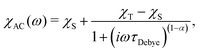 | (1) |
where
τDebye−1 is the relaxation rate,
ω is the angular frequency of the AC field and
χT and
χS are the isothermal and adiabatic susceptibilities, respectively. The
α parameter (0 <
α ≤ 1) describes the width of the distribution of relaxation times, with
α = 0 corresponding to an infinitely sharp distribution (the Debye model). AC methods typically have a lower frequency limit of
ca. 0.1 Hz, and therefore cannot accurately characterise SMMs with rates slower than ∼1 s
−1.
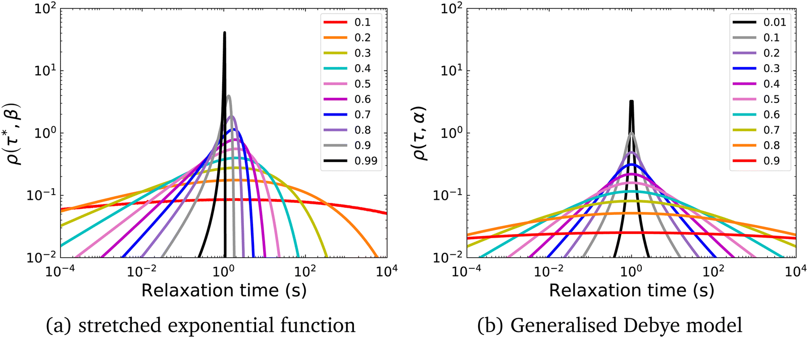
To measure magnetisation relaxation rates at longer timescales, the technique of direct current (DC) magnetisation decay is often employed.1 In this approach, the sample is magnetised in a large external field, which is then quickly switched off, and the magnetisation versus time is measured. While any single molecule in a sample is expected to show a mono-exponential magnetisation decay, ensemble effects generally lead to the appearance of multi-exponential decays,8,9 which are commonly modelled via a stretched exponential function (SEF):
| | 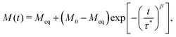 | (2) |
where
τ*
−1 is the “characteristic relaxation rate”,
M0 and
Meq are the initial and equilibrium magnetisation, respectively, and the stretch parameter 0 <
β ≤ 1 describes the multi-exponential character, with
β = 1 corresponding to mono-exponential decay. Historically in the SMM community, the values of
τDebye−1 and
τ*
−1 have been taken as the relaxation rates of the SMM and
α and
β were simply ignored. However, these parameters encode vital information about the distribution of relaxation rates in the experimental data (
Fig. 1).
10 For instance,
β in
eqn (2) is known to represent distributions in samples when the SEF is used for the analysis of supercapacitor discharge,
11,12 X-ray photon correlation spectroscopy,
13 and can indicate the onset of long-range-order in μ-SR measurements.
14 The stretched exponential function is also used extensively in the study of spin-glass phenomena
15,16 and NMR measurements.
8,17,18 Elsewhere, a lack of understanding of the physical relevance of the
β parameter has stifled advancement in the lifetime of batteries.
19
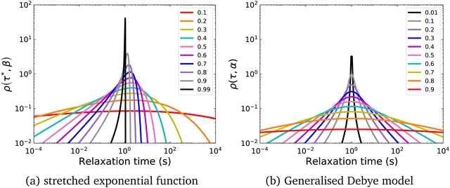 |
| | Fig. 1 Probability distribution of relaxation times in the logarithmic domain (ρlog) for (a) the stretched exponential function with τ* = 1 s and (b) the Generalised Debye model with τDebye = 1 s and different indicated values of β and α respectively. | |
Recently, using the known analytical distribution function implied by the Generalised Debye model,20 we developed a method for approximating estimated standard deviations (ESDs) of magnetic relaxation rates from the α parameter.10 Accounting for experimental ESDs gives an indication of how strongly trends in the data can be relied upon to avoid over-interpretation, and indeed important information on SMM magnetisation dynamics can be gleaned from the behaviour of the distribution width as a function of temperature and/or magnetic field.21
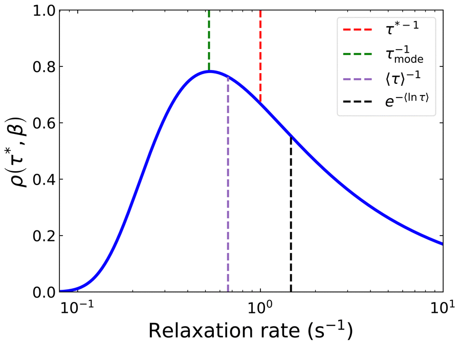
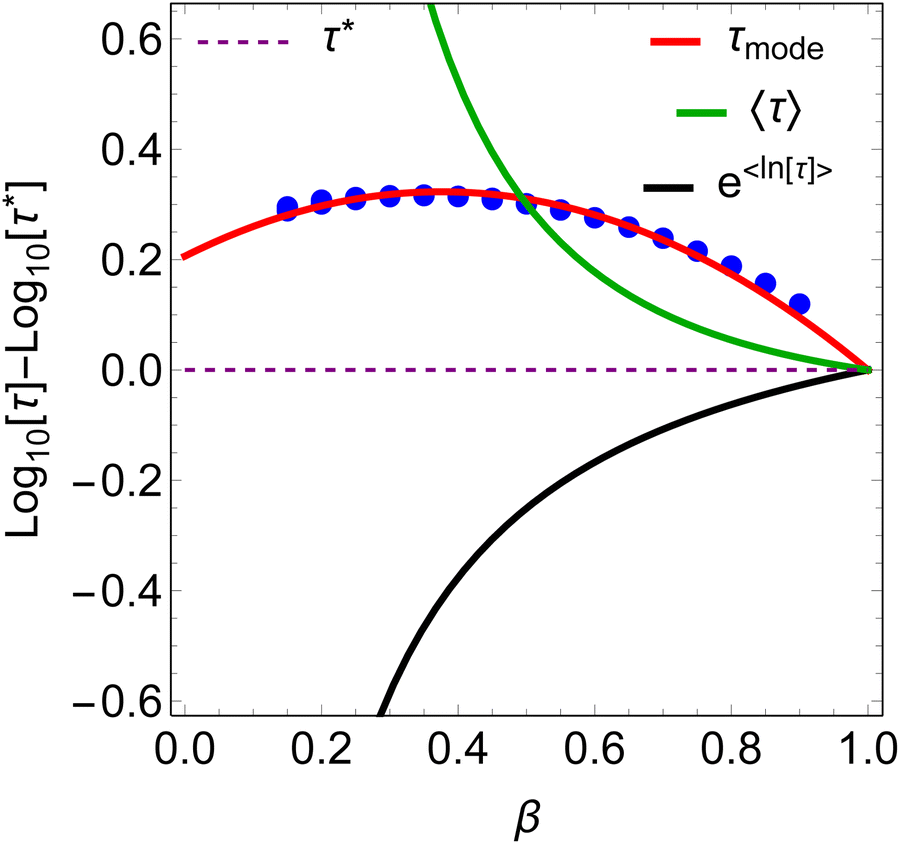
In a similar vein, we previously approximated ESDs for rates derived from the SEF, using the β parameter22 and the SEF distribution function.23 In that work we followed literature precedent, and our own bias, and ascribed particular importance to the characteristic relaxation rate τ*−1, using it as the central value around which to define symmetric ESDs on a logarithmic scale. However, unlike the Generalised Debye model, the distribution of the SEF is asymmetric (Fig. 1); hence, the “centre” of the distribution changes with its width. Thus, as well as τ*, one may consider the peak of the distribution (the mode), τmode, and two calculated expectation values of τ, evaluated on a linear (〈τ〉) or logarithmic scale (e〈ln[τ]〉) as being indicative of “the relaxation rate” (Fig. 2). These measures of τ diverge when β < 1 (Fig. 4), and given that low values of β (0.4–0.7) are common for SMMs, particularly those with extremely slow relaxation rates,4,5,24,25 there is a drive to assess which of these values most reliably correspond to “the experimental relaxation rate”.
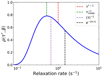 |
| | Fig. 2 Distribution of the stretched exponential function with τ* = 1 s and β = 0.6 showing the four measures of the rate: τ*−1, τmode−1 (eqn (7)), 〈τ〉−1 (eqn (8)15), e−〈ln[τ]〉 (eqn (9)26). | |
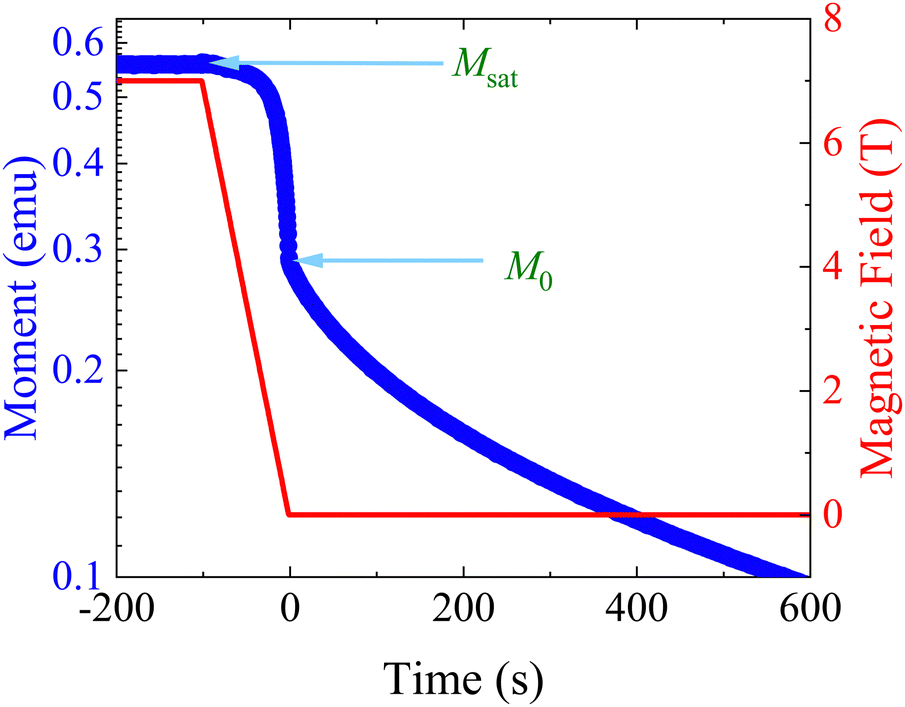
Separately, the experimental process of measuring magnetisation decays is not ideal. Most magnetometers in use by the community employ a superconducting magnet, which constrains the maximum sweep rate to <0.1 T s−1 and hence the switch-off time of the saturating field is non-negligible (Fig. 3). If the magnetic relaxation timescale τ is short compared to the sweep rate of the instrument, many of the moments in the sample would have equilibrated in this time period and their relaxation is not observed. This does not present an issue if there is no distribution of relaxation timescales in the sample, as a mono-exponential decay appears mono-exponential at all points in the decay. However, as β decreases and the distribution becomes broader, the initial part of the decay becomes increasingly faster relaxing—reflected in increased ρ(τ*,β) at short relaxation times in Fig. 1a. Much of the sample would therefore have equilibrated before the decay measurement has begun, skewing the decay trace to the more slowly relaxing part of the sample. Exacerbating this effect is that often the first measured point is subject to a wait command until “field stability”, which can take a further 10 s before measurements can begin (Fig. S36a and Table S10, ESI†). Another experimental concern is that the target field may not be accurate—superconducting magnets are well-known to trap residual fields, meaning that “zero-field” is not necessarily zero: hence, field calibration is essential for accurate data. Furthermore, in the case of samples with very slow dynamics it may not be practical to measure the entire decay curve, and in the presence of distributions this has an impact on the results. Finally, the application of eqn (3) for fitting the data (i.e. fixing or freely fitting certain parameters) also affects the extracted values of τ* and β. Therefore, here we will examine all of these experimental considerations and propose a set of guidelines to obtain high-quality magnetisation decay data.
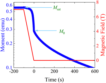 |
| | Fig. 3 Example DC decay measurement. Samples are saturated at high magnetic field before the field is swept to the target field. In a Quantum Design MPMS3 the fastest field sweep rate is 700 Oe s−1, such that it takes ≈100 s to go from 7 T to 0 T. The x-axis is set to t = 0 s at M0, and Meq is not shown on this scale. | |
In order to benchmark the quality of our magnetisation decay experimental design, fitting and interpretation, we need a reliable standard. Ideally this would be AC susceptibility, where τmode = 〈τ〉 = e〈ln[τ]〉 = τDebye. However the slowest accessible AC timescale is too fast to compare to DC decay methods. Our solution is to employ the recently-proposed long-timescale AC susceptometry-like “waveform” experiment.27 This technique employs a low-amplitude oscillating square-wave magnetic field, that drives slow oscillations in the magnetisation, resulting in a shark-tooth-like magnetisation versus time profile (see for example Fig. S1e, ESI†). Fourier transform of the time-domain data allows determination of the effective in-phase (χ′) and out-of-phase (χ′′) susceptibility components at the fundamental frequency: neglecting of the higher-order Fourier components is akin to the lock-in detection of standard regular AC susceptibility measurements. The resulting data can then be modelled in the same way as AC data (e.g. using eqn (1)). Because the magnitude of the drive field is small—Hilgar et al. proposed ±8 Oe, and we use this magnitude herein—the practically-accessible frequency range is of the order of 10−5–10−1 Hz, constrained on the fast end only by the sweep rate and the discrete time taken to perform a measurement. Thus, this technique provides a bridge to benchmark the accuracy of our magnetisation decay experiments and our interpretations. We note that the waveform technique will not supplant use of magnetisation decay experiments, because it is impractical to measure enough waveform data for the slowest relaxing samples, and a single DC decay is often the most that can be measured in the instrument time available.
This paper is arranged as follows: first, we determine an approximation for τmode−1 from the SEF; second, we propose guidelines for measuring magnetisation decays; third, we compare the temperature dependence of τDebye obtained from the waveform technique to different measures of τ extracted from magnetisation decay fits (τ*, τmode, 〈τ〉 and e〈ln[τ]〉) to determine the most accurate measure of τ for DC decay measurements, including the different variables in the fitting procedure of the SEF to the experimental data. Our experiments are performed on the [Dy(Dtp)2][Al{OC(CF3)3}4] (Dtp = P(Ct BuCMe)2) SMM in zero DC field. This compound has been extensively characterised by Evans et al.,22 and shown to be ideally suited for comparison of these two techniques due to its relaxation dynamics straddling measurement timescales for both waveform and DC decay techniques, and because it shows 0.46 < β < 0.86.
2 Theory
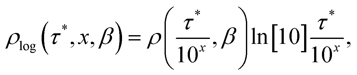
In a DC magnetisation decay measurement, the magnetic moment vs. time trace is typically fit to the SEF described by eqn (2). The probability density distribution of the SEF is given by:23| | 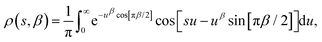 | (3) |
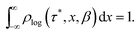
where s = τ*/τ and u = −ix, and the normalisation condition is given by:| |  | (4) |
To represent the distribution on a logarithmic scale, we convert eqn (3) to the log[τ] domain, where x = log[τ] (herein we use log to indicate log10 and ln to indicate loge):| |  | (5) |
| |  | (6) |
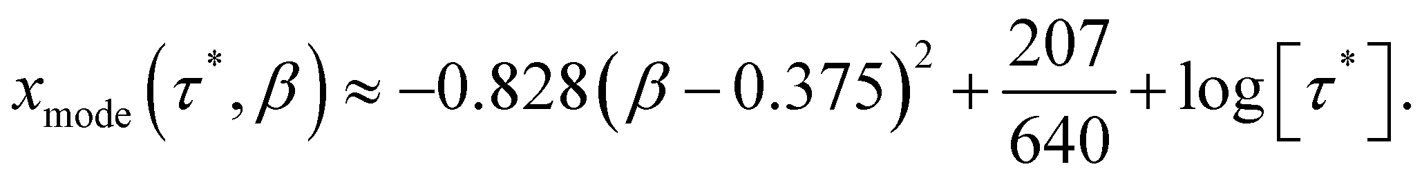
To find τmode of the SEF distribution, we numerically find the values of x for which ρlog(τ*,x,β) is maximum for various values of β, in the range − 4 < log[τ*] < 4. The β-dependence of τmode is well approximated by a parabolic function (Fig. 4; eqn (7)), where we see no effect of τ*. Thus, we define τmode = 10xmode. Note that the constant term in eqn (7) enforces xmode → log[τ*] as β → 1.| | 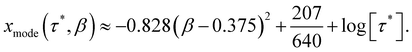 | (7) |
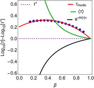 |
| | Fig. 4
β-Dependence of the four measures of τ relative to τ*. Blue circles are the mode of the SEF distribution for −4 < log[τ*] < 4; there is no observable dispersion. | |
The SEF distribution has exactly defined values for the expectation value of 〈τ〉15 and 〈ln[τ]〉:26
| | 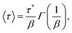 | (8) |
| |  | (9) |
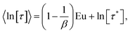
where
Γ is the Gamma function and Eu = 0.5772… is the Euler constant. When the distribution of relaxation times is large (
i.e. β is small for the SEF, or
α is large for the Generalised Debye model), the concept of “the relaxation time”
τ begins to lose physical meaning. However, even at relatively high values of
β, the different measures of
τ for the SEF diverge (
Fig. 4). The expectation value 〈
τ〉 is always longer than
τ*, while e
〈ln[τ]〉 is always shorter than
τ* and both rapidly diverge from
τ* at
β < 0.5. The value of
τmode is also larger than
τ*, but goes through a maximum at
β ≈ 0.4, where
τmode is approximately twice as large as
τ* (
Fig. 4). The staggering difference in
β-dependence for the different measures of
τ is likely to have significant implications on the temperature-dependence of magnetic relaxation rates, as
β values commonly vary with temperature; this could have important consequences for the accurate chemical interpretation of relaxation dynamics.
3 Experimental details
Magnetic measurements were performed on a Quantum Design MPMS3 SQUID magnetometer. A 31.5 mg polycrystalline sample of [Dy(Dtp)2][Al{OC(CF3)3}4] (from the same batch as synthesised and characterised by Evans et al.)22 was crushed with a mortar and pestle under an inert atmosphere, and then loaded into a borosilicate glass NMR tube along with 15.9 mg powdered eicosane, which was then evacuated and flame-sealed to a length of ca. 5 cm. The ampoule was loaded into a straw that was fixed to a translucent glass-reinforced polycarbonate adaptor attached to a carbon-fibre rod.
Details of magnetisation decay measurements are given in Section 4.2. Waveform measurements were performed as a function of frequency and temperature (2–23 K). The same method developed by Hilgar et al.27 was used, but with a sweep rate of 700 Oe s−1 and each square-wave period repeated five times for all temperatures apart from the 36 μHz measurement at 4 K, where 3 square-wave periods were used. Between 7 and 11 unique frequencies of the driving square-wave magnetic field were used at each temperature. The magnet was reset before the measurements were performed to ensure that the superconducting magnet did not contain residual fields. In- and out-of-phase susceptibility components were extracted from the data using the Super package in Matlab.27 Fitting of the frequency-dependence of the susceptibility components was performed in Mathematica.28 Fitting of the relaxation profiles was performed in CC-FIT2 using the relaxation module.10
4 Results and discussion
4.1 Benchmark waveform data
We have measured magnetic relaxation rates for [Dy(Dtp)2][Al{OC(CF3)3}4] between 2–23 K using the waveform technique. The waveform data is generally good quality, although we note some noise in the 36 μHz and 69 μHz data sets at 2 K (Fig. S1a and c, ESI†). The selected square-wave frequencies at each temperature contain sufficient data to cover a complete Cole–Cole curve and thus accurately characterise the relaxation processes.1 The isothermal frequency-dependence of the in-phase and out-of-phase susceptibility data were fit to the Generalised Debye model (eqn (1)) in Mathematica to obtain τDebye and α with good agreement between the fit and the data (Fig. S29–S31, ESI†). The resulting temperature dependence of τDebye−1 was fitted to:| | | log[τ−1] = log[10−Ae−Ueff/T + 10RTn + 10−Q], | (10) |
which encapsulates the Orbach (10−Ae−Ueff/T, τ0 = 10−A), Raman (10RTn, C = 10R) and quantum tunneling of magnetisation (τQTM = 10Q) contributions to the overall relaxation rate.2 The resultant fit is given in Fig. 5 and shows good agreement between the fitted model and data.
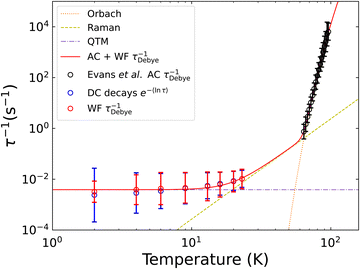 |
| | Fig. 5 Comparison of τDebye−1 and e−〈ln[τ]〉 extracted from Waveform and DC decay measurements of [Dy(Dtp)2][Al{OC(CF3)3}4]. The waveform (red) and AC data[22] (black) are fitted to eqn (10), with each contribution represented as a dotted line. Fitted parameters are given in Table 2. | |
4.2 Magnetisation decay experimental design
4.2.1 Field calibration.
An ideal magnetisation decay measurement captures the magnetic moment of a sample as a function of time, M(t), from when the saturating field is instantaneously switched to the target field until the moment has reached its equilibrium value. The magnetic field reported by a superconducting magnet system can deviate from the real magnetic field in the sample chamber by tens of Oe, especially at low fields, due to pinned magnetic flux lines and flux movement.29 Known techniques to reduce the remanence of the magnet, such as oscillating to the target field or resetting the magnet, are incompatible with the premise of the magnetisation decay measurement. The remanent properties of the magnet are reproducible for a given field charging sequence, so the magnet can be calibrated with a standard sample for a particular experiment, and the target field set to achieve the desired real field.30 Whilst is it possible to use the ultra low field (ULF) option to cancel the pinned flux, this requires calculating all the currents in the ULF coils needed to completely cancel the field, and assumes the currents will not change significantly once the superconducting magnet has been turned on; there is no assurance that this will provide any advantage over the simpler Pd calibration protocol. Therefore, the magnetic field applied by the superconducting magnet was calibrated at 298 K using the standard palladium sample with known magnetic moment. Sweeping from +70 kOe to “zero field”, in fact corresponded to −22 Oe or −23 Oe, and thus all magnetisation decays were performed in a target field of +22 Oe or +23 Oe to correct for this. Precisely zero magnetic field is essential if relaxation rates are highly sensitive to applied fields, which is the case for single-molecule magnets, and allows Meq to be independently defined and fixed: zero in zero field, or accurately predicted for specific temperatures and fields using an experimentally-calibrated model Hamiltonian.
4.2.2 Measurement settings.
To evaluate when the zero-field condition is reached and which method of data collection (vibrating-sample magnetometer (VSM) or DC modes) imposes the least amount of “dead time”, short magnetisation decay measurements were performed at 13 K. The sample was first cooled in zero-field then magnetised at +7 T for 30 minutes before the field was swept to the calibrated target of +23 Oe at 700 Oe s−1, and held for 15 min. The field and field status (stable or sweeping) were recorded at 0.25 s intervals using the logging function. This field sequence was repeated for each of the following settings: VSM mode with a peak amplitude of 1 mm and averaging time of 0.5 s with either sticky autorange or fixed range settings; or DC mode with fixed range, a 30 mm scan length and either 1 or 4 s scan time. For each measurement method, we examined both continuous measurement throughout the field sequence, or measurement only after stable field was achieved.
Using VSM mode allows for a very high density of points, which is important when the moment changes quickly at the beginning of the decay and at high temperatures (Fig. S37, ESI†). Fast DC scans (1 s scan time) can also result in a reasonably high density of data points if VSM is unavailable (Fig. S36, ESI†). Users should take care to avoid frictional heating, which can be an issue for VSM and the fast 1 s DC scans, particularly at low temperatures; here, keeping the instrument well-maintained (clean sample chamber, smooth sample rod bearings, sample rod and mount straight and not rubbing inside the sample space) and using smaller VSM amplitudes or slower DC scans can help reduce this effect if it arises. It is necessary to use autoranging, as the magnitude and time dependence of the magnetic moment of a sample is not known in advance. Unfortunately, however, we find this results in gaps and jumps in the decay curve (Fig. S37a and b, ESI†) when the magnitude of the moment falls at the boundary of the SQUID voltage ranges, causing the autorange logic to bounce between two options (leading to missing datapoints) until the moment has dropped far enough such that a single range is suitable. When using autoranging for DC scans, we find that the timestamp of the first point for a new range is reported incorrectly and these points must be discarded.31 It is possible to avoid this problem using sequential fixed range measurement commands at different points of the decay curve.
4.2.3 Approaching target field.
We now examine the approach to target field and whether a “wait for stable field” command is required; the point at which the target field is reached will define the start of the decay. Logging the field and field status as the magnet sweeps from +70 kOe to zero field (calibrated) shows the stable status is reached 1.5–2.3 s after reaching the target field but the field is consistently within ±0.5 Oe of the final value as it stabilises (Fig. S36, S37 and Table S10, ESI†). We measured the magnetic moment of the sample continuously through the field change to experimentally interrogate when the zero field condition was reached by finding when d3M(t)/dt3 = 0 (Fig. S33, ESI†). These data indicate zero field is achieved within ≈ 0.7 s of the log recording the target field. To capture a full decay in the target field, one must measure through the field change and use the first measured data point at the target field to define t = 0 and M0.
Continuously measuring in VSM mode is the preferred measurement method as the first recorded datapoint is closest to when the target field is reached: within 0.6 s of both the instrumental log reaching the target field and the third-derivative condition at all temperatures (<1.3 s when data points missing around zero field, Fig. S34 and S35, ESI†). A “wait for stable field” command is not required, and it introduces an ∼8 s delay in acquiring the first point at the target field (VSM mode) and artifacts in the first few points if autoranging is used (Table S10 and Fig. S37, ESI†).
In the event that a significant portion of the magnetisation has decayed before reaching target field (for example M0 < 0.1Msat) or in cases with very small β, the fast relaxing components will not be observed in the decay trace. As such, the extracted relaxation time will be too long, which could explain the very large discrepancy between τDebye and τ* extracted from waveform and DC decay measurements of [K(L)][Er(COTTBS2)2] (COTTBS2 = 1,4-(tBuMe2 Si)2C8H6), L = (DME)2 (DME = ethylene glycol dimethyl ether), 18-crown-6 and 2.2.2-cryptand.32 For compounds that relax this quickly, we recommend the waveform method, especially in the case of very broad distributions. The required measurement time will not pose an issue in such cases.
4.2.4 Measurement time.
We will discuss for how long a decay should be recorded in Section 4.3.1: as this cannot be known in advance of measurement, we recommend interactive measurements with far longer than necessary recording times that can be terminated when sufficient data has been acquired.
4.2.5 Magnetisation decay protocol.
Full magnetization decays were recorded at the same temperatures as waveform measurements (2, 4, 6, 9, 13, 16, 20 and 23 K) to provide data for determining optimal analysis methods. The sample was first cooled in zero-field to 2 K. The sample moment was saturated for 30 mins at +7 T, then swept to the calibrated target of +22 Oe at 700 Oe s−1 and held for 6 hours. The sample moment was measured continually throughout the saturation, field sweep and decay at zero-field using the VSM mode with a peak amplitude of 1 mm, averaging time of 0.5 s and sticky autorange setting. After the measurement time had elapsed the temperature was increased to the next target and the previous steps were retaken. For all other temperatures a measurement time of 5 hours at zero-field was used. Fitting of the magnetisation decays was performed with a Python script.
4.3 Data analysis
4.3.1 Magnetisation decays.
We now investigate how to best analyse magnetisation decay data, with the goal of finding the best reproduction of the waveform τDebye dataset. We fit the DC decay data to a generalised version of eqn (2):| | 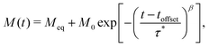 | (11) |
where toffset is included to account for possible decay before t = 0 during switching of the magnetic field. Variations of this model were attempted with M0 fixed to the first measured point at target field or freely fitted; toffset fixed to zero or freely fitted; and Meq fixed to the last point, fixed to zero, or freely refined (Table S15, ESI†). All possible combinations of fixing and freely fitting these parameters were performed on the full DC decay datasets (Fig. S54–S77, ESI†).
We find, in all cases, that the measured magnetisation data for [Dy(Dtp)2][Al{OC(CF3)3}4] deviate from a stretched exponential model at very long timescales, where M(t) ≲ 0.01M0. Attempts to model dynamics at these long timescales using a second stretched exponential or mono-exponential function were unsuccessful. Whilst including these data in the fitting process does not negatively impact the fitting of eqn (11) due to the small moment at long timescales, it does not add anything to the model. Therefore, we repeated the full fitting process with datasets trimmed to only include M(t) ≥ 0.01M0 (Fig. S78–S101, ESI†), which gives equivalent parameters to fitting the whole decay trace. To investigate the impact of fitting incomplete decays, as may be required for very slow relaxing samples, we trimmed the decay data at 0.05M0 and 0.1–0.9M0 in steps of 0.1 (i.e. 95% and 90–10% of the decay included), and repeated the fits with Meq fixed to zero or freely fitted (for this test toffset was fixed to zero and M0 fixed to the first measured point at target field). We find that allowing Meq to refine freely quickly results in unphysically-large values of Meq, and diverging values of τ* and β as less of the decay is included (Fig. S39–S45 and Tables S11, Table S14, ESI†). In contrast, fixing Meq results in much more stable fits33 (Fig. S51 and S53, ESI†), and is absolutely necessary when fitting incomplete decays. We recommend measuring the decay to 0.01M0 and fitting the trace with Meq fixed; minimally, measuring to 0.1M0 and fitting with fixed Meq is associated with an acceptable error of 5% in both τ* and β. Measuring the decay to 0.01M0 corresponds to a measurement time of t ≈ 10τ* (Fig. S51, ESI†), which is consistent with the calculated maximum recommended T1 measurement time for non-exponential (i.e. stretched exponential) relaxation in solid state NMR measurements.8
Using the M(t) ≥ 0.01M0 decay traces, we now compare the options of fixed or free parameters in eqn (11), along with all measures of τ (τmode, 〈τ〉, e〈ln[τ]〉 and τ*), to find which combination provides the closest match to the waveform dataset (Fig. S104 and S105, ESI†). All methods that allow free fitting of M0 are generally in poor agreement with the waveform results, showing a downturn for most measures of τ at low temperatures or show wildly diverging values at high temperatures (Fig. S104, ESI†). Thus, M0 should be defined by the first point in the target field, toffset should be set to zero and using eqn (2) is sufficient; gratifyingly, this corresponds to the methodology employed by most experimental groups, including ourselves, to date. As we only fit M(t) ≥ 0.01M0, then Meq should either be free or fixed to the target value (which here is Meq = 0 as the target field is calibrated to zero) and not fixed to the last measured point. Allowing Meq to refine freely gives very similar parameters (<5% variation; Tables S11 and S12, ESI†) compared to when it is fixed to zero (Table 1).
Table 1 Parameters extracted from fitting DC decay data to 0.01M0 for [Dy(Dtp)2][Al{OC(CF3)3}4] using eqn (11) with M0 fixed to the first point, Meq = 0 and toffset = 0. Values of τ* and β were freely fit
| Temperature (K) |
M
0 (emu) |
β
|
τ* (s) |
| 2 |
0.298 |
0.466 |
814.3 |
| 4 |
0.287 |
0.574 |
534.2 |
| 6 |
0.273 |
0.627 |
410.9 |
| 9 |
0.253 |
0.675 |
302.8 |
| 13 |
0.214 |
0.737 |
222.1 |
| 16 |
0.187 |
0.778 |
177.3 |
| 20 |
0.153 |
0.827 |
132.1 |
| 23 |
0.131 |
0.857 |
106.4 |
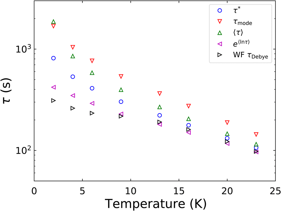
The final option is the choice of the most appropriate measure of τ to replicate τDebye as closely as possible (Fig. 6). It is clear that e〈ln[τ]〉 is consistently in the best agreement with τDebye across the whole temperature range, and therefore we contend that e〈ln[τ]〉 should be used as the experimental definition of the magnetic relaxation time for the SEF in conjunction with magnetisation decay experiments.
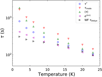 |
| | Fig. 6 Comparison of relaxation rate extracted from waveform measurements of [Dy(Dtp)2][Al{OC(CF3)3}4] to the four metrics of the rate that were obtained from fitting the DC decay data to 0.01M0. M0 is fixed to the first measured point, toffset = 0 and Meq is set to target. α and β are freely fitted. The parameters are shown in Table 1. | |
4.3.2 Defining ESDs.
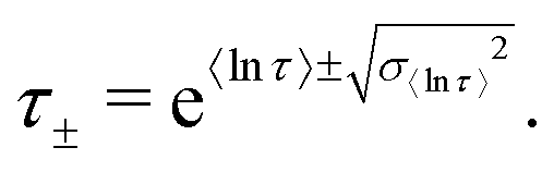
Having identified the most reliable measure of τ as e〈ln[τ]〉, we now address the definition of estimated standard deviations (ESDs). For 〈ln[τ]〉 in the stretched exponential function, the variance is defined exactly:26| |  | (12) |
and therefore the standard deviation of 〈ln[τ]〉 is given by the square root of eqn (12), and the limits of one ESD in τ are given by:| |  | (13) |
We note that the deviation between e〈ln[τ]〉 and τ* will always lie within one ESD of e〈ln[τ]〉 because the square root of the variance (eqn (12)) is greater than the absolute difference between 〈ln[τ]〉 and τ* from eqn (9).
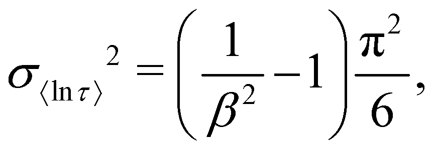
Previously we used numerically-approximated ESDs for the Generalised Debye model.10 Logarithmic moments have been shown to be an appropriate metric for comparing different distributions,26 and so, similar to the SEF model, the variance of 〈ln[τ]〉 can be used (recall that for the Generalised Debye distribution τDebye = e〈ln[τ]〉). In the Generalised Debye model the variance of 〈ln[τ]〉 is defined exactly:26
| |  | (14) |
The ESDs defined by
eqn (14) and (13) are in good agreement with the numerically derived ESDs
10 over the whole range of
α (Fig. S115, ESI
†). We have updated the ESD definitions for both the Generalised Debye and SEF models in CC-FIT2
10 to those described by
eqn (12)–(14). Finally, we can compare
τ−1 with ESDs between waveform and decay measurements for [Dy(Dtp)
2][Al{OC(CF
3)
3}
4] to show that they are in excellent agreement (
Fig. 5). The exception is at 2 K, where the ESDs for the waveform data are narrower than for the decay-derived data and the other waveform data at higher temperatures—this is attributed to noise in some of the 2 K waveform datasets.
4.4 Consequences for chemical interpretation
Our new definitions have important ramifications on the extracted parameters and their chemical interpretation. The temperature-dependence of τ*−1 for [Dy(Dtp)2][Al{OC(CF3)3}4] suggests that only a Raman relaxation mechanism is active at low temperature owing to the linearity of the plot (Fig. S112 and ref. 22). However, the waveform τDebye−1 and decay e−〈ln[τ]〉 rates show a levelling off at low temperature, suggesting the presence of QTM, consistent with the hysteresis data.22 Fitting the temperature-dependence of τDebye−1 or e−〈ln[τ]〉 to eqn (10) gives chemically sensible parameters (Fig. 5, Fig. S110 and Table 2, ESI†), including a Raman exponent of ca. 4 compared to the originally-reported value of ca. 1.22
Table 2 Parameters obtained from fitting relaxation rates obtained from AC susceptibility measurements of [Dy(Dtp)2][Al{OC(CF3)3}4]22 along with those extracted from Waveform or DC decay measurements performed on [Dy(Dtp)2][Al{OC(CF3)3}4] to eqn (10). The resultant fits are shown graphically in Fig. 5 and Fig. S106
| Parameter |
DC decays |
Waveform |
|
τ* |
e〈ln[τ]〉 |
τ
Debye
|
|
U
eff (K) |
1823(28) |
1842(22) |
1845(20) |
|
A(τ0 = 10A s−1) |
−12.0(0.16) |
−12.10(0.12) |
−12.11(0.11) |
|
R(C = 10R s−1 K−n) |
−6.95(0.42) |
−7.34(0.34) |
−7.52(0.31) |
|
n
|
3.56(0.30) |
3.84(0.22) |
3.95(0.20) |
|
Q(τQTM = 10Q s−1) |
2.591(0.053) |
2.424(0.045) |
2.413(0.031) |
Low β values will lead to the largest deviation between τ* and e〈ln[τ]〉, and these are typically associated with the QTM region: hence, many QTM rates in the literature are likely inaccurate. McClain et al. reported four Dy SMMs with the general formula [Dy(C5iPr4R)2][B(C6F5)4] (R = H, Me, Et, iPr):5 using the reported τ* and β values, the QTM tunnelling times change by 20–34% (Table 3). However, using reported τ* and β values may not be sufficient. The current best dysprosocenium SMM, [Dy(C5iPr5)(C5Me5)][B(C6F5)4] has a reported 2 K relaxation time of τ* = 104.40 s or ca. 7.0 hours with β = 0.553, and M0 and Meq were allowed to vary freely in fitting.4 Using the reported parameters, e〈ln[τ]〉 = 104.20(0.67) s (4.4 hours) but refitting the experimental data with M0 fixed to the first point measured at zero-field and Meq = 0 (Fig. S116 and S117, ESI†) gives e〈ln[τ]〉 = 104.29(0.62) s (5.4 hours). A necessary step in progressing towards chemical control of QTM is the accurate determination of relaxation times and these large variations stress the need for consistency in fitting and interpretation of magnetisation decays. The changes to how one should analyse AC susceptibility, waveform and DC decay data have been updated into CC-FIT2.10 We also strongly encourage the SMM community to publish their full magnetic datasets, to enable re-analysis of magnetisation decay data.
Table 3 Comparison of τQTM values of [Dy(C5iPr4R)2][B(C6F5)4] reported by McClain et al.5 to e〈ln[τ]〉 calculated using the reported τ* and β values
| R |
McClain et al. τQTM (s) |
e〈ln[τ]〉τQTM (s) |
| H |
102.64 |
102.56(0.39) |
| Me |
103.39 |
103.27(0.49) |
| Et |
102.65 |
102.52(0.50) |
|
i
Pr |
103.07 |
103.00(0.38) |
We will now discuss some general considerations from our experiences. Magnetisation decays are a time-based measurement, and a distribution of relaxation rates will result in a decay curve that changes shape with elapsing time, so any relaxation not captured in the experiment will skew the extracted τ* and β parameters. This gives an upper bound on the measureable distribution at τ−1 ∼ 0.1 s−1, and will generally occur at higher temperatures where the fast-relaxing components have already equilibrated before the first measured point. This bias towards long-timescales is not an issue for waveform measurements, as the presence of faster rates can be inferred by fitting the frequency dependence of the oscillating magnetisation. Thus, even when using e〈ln[τ]〉, a discrepancy may arise with τDebye waveform rates, and the decay-based rates may not be reliable.31 It may also occur that the distribution of rates in a sample is significantly skewed, and the waveform data are not well represented by a symmetric Generalised Debye distribution: one alternative is to use the Havriliak–Negami model7 which also has a known expectation value and variance.26 For compounds that are required to be modelled like this then we expect that e〈ln[τ]〉 will provide the best measure to compare relaxation times in both cases.
5 Conclusion
Herein we have re-evaluated the underlying distribution implied by use of the stretched exponential function for magnetisation decay data. We have derived an expression for τmode, investigated how different measures of τ change with β and identified the limitations of interpreting τ in the case of broad distributions.
We have established new guidelines for the collection, fitting and interpretation of magnetisation relaxation times derived from DC decay measurements. After calibrating the magnet, we advocate continuous VSM measurement through the field change and in the target field until 99% of the decay has elapsed (the moment has reduced to at least 0.01(M0−Meq)), or 90% of the decay for very slow relaxing samples. If VSM mode is not available, then continuous DC scans with a short scan time are the second preference. Magnetisation decay data should be fit to eqn (2) with M0 fixed to the first point measured in the target field and Meq fixed to the calculated target value; only if 99% of the decay is measured can Meq be reliably freely fit. The relaxation time from magnetisation decays is best described by e〈ln[τ]〉 (eqn (9)), with ESDs defined by the logarithmic variance (eqn (13)). This measure of τ is commensurate with τDebye derived from the waveform technique of Hilgar et al., and results in a chemically reasonable interpretation of the temperature-dependence of relaxation rates for [Dy(Dtp)2][Al{OC(CF3)3}4], unlike the previous use of τ* alone.
We find that both DC magnetisation decay and long-timescale AC waveform techniques can be recommended for measurement of relaxation data. Magnetisation decay measurements are limited by the time taken to change the field, restricting the recording of faster rates, and potentially biasing broad relaxation distributions. On the other hand, the square-wave method is the gold standard, but as multiple oscillations are required on a time-scale appropriate for the magnetisation relaxation time, the required experiments can be incredibly long.
6 Research data
The magnetisation decay traces, waveform datasets and Python code used to analyse the decay traces for [Dy(Dtp)2][Al{OC(CF3)3}4] can be obtained via FigShare at https://doi.org/10.48420/22203130. CC-FIT2 is available at https://gitlab.com/chilton-group/cc-fit2.
Author contributions
WJAB and GKG identified the problem and developed the methodology. WJAB performed and analysed the magnetometry measurements on [Dy(Dtp)2][Al{OC(CF3)3}4]. GKG collected and analysed magnetometry data for the measurement protocol. PE synthesised [Dy(Dtp)2][Al{OC(CF3)3}4]. NFC developed the numerical models. JGCK updated the CC-FIT2 code to be compatible with the new protocol. WJAB, GKG and NFC wrote the manuscript together. NFC and DPM supervised the work.
Conflicts of interest
There are no conflicts to declare.
Acknowledgements
We thank The University of Manchester, the European Research Council (ERC-2019-STG-851504 to NFC and ERC-2018-CoG-816268 to DPM) and The Royal Society (URF191320 to NFC) for funding. We acknowledge the EPSRC UK National Electron Paramagnetic Resonance Service for access to the SQUID magnetometer (EP/S033181/1). We acknowledge Dr Sophie Corner for sample preparation, Mr Adam Brookfield for technical support and Dr Daniel Reta for updating the CC-FIT2 code. We thank Prof. David Collison, Dr Andrea Mattioni, Mr Jakob Staab and Ms Lucia Corti for useful discussions.
Notes and references
-
D. Gatteschi, R. Sessoli and J. Villain, Molecular Nanomagnets, Oxford University Press, 2006 Search PubMed.
-
M. J. Giansiracusa, G. K. Gransbury, N. F. Chilton and D. P. Mills, Single-Molecule Magnets, Encyclopedia of Inorganic and Bioinorganic Chemistry, Wiley, 2021, pp. 1–21 Search PubMed.
- C. A. P. Goodwin, F. Ortu, D. Reta, N. F. Chilton and D. P. Mills, Molecular magnetic hysteresis at 60 kelvin in dysprosocenium, Nature, 2017, 548, 439–442 CrossRef CAS PubMed.
- F.-S. Guo, B. M. Day, Y.-C. Chen, M.-L. Tong, A. Mansikkamäki and R. A. Layfield, Magnetic hysteresis up to 80 kelvin in a dysprosium metallocene single-molecule magnet, Science, 2018, 362, 1400–1403 CrossRef CAS PubMed.
- K. R. McClain, C. A. Gould, K. Chakarawet, S. J. Teat, T. J. Groshens, J. R. Long and B. G. Harvey, High-temperature magnetic blocking and magneto-structural correlations in a series of dysprosium(III) metallocenium single-molecule magnets, Chem. Sci., 2018, 9, 8492–8503 RSC.
- C. A. Gould, K. R. Mcclain, D. Reta, J. G. C. Kragskow, D. A. Marchiori, E. Lachman, E.-S. Choi, J. G. Analytis, R. D. Britt, N. F. Chilton, B. G. Harvey and J. R. Long, Ultrahard magnetism from mixed-valence dilanthanide complexes with metal–metal bonding, Science, 2022, 375, 198–202 CrossRef CAS PubMed.
- C. V. Topping and S. J. Blundell, A.C. susceptibility as a probe of low-frequency magnetic dynamics, J. Phys.: Condens. Matter, 2019, 31, 013001 CrossRef CAS PubMed.
- A. Narayanan, J. S. Hartman and A. D. Bain, Characterizing Nonexponential Spin-Lattice Relaxation in Solid-State NMR by Fitting to the Stretched Exponential, J. Magn. Reson., Ser. A, 1995, 112, 58–65 CrossRef CAS.
- A. Chiesa, F. Cugini, R. Hussain, E. Macaluso, G. Allodi, E. Garlatti, M. Giansiracusa, C. A. P. Goodwin, F. Ortu, D. Reta, J. M. Skelton, T. Guidi, P. Santini, M. Solzi, R. De Renzi, D. P. Mills, N. F. Chilton and S. Carretta, Understanding magnetic relaxation in single-ion magnets with high blocking temperature, Phys. Rev. B, 2020, 101, 174402 CrossRef CAS.
- D. Reta and N. F. Chilton, Uncertainty estimates for magnetic relaxation times and magnetic relaxation parameters, Phys. Chem. Chem. Phys., 2019, 21, 23567–23575 RSC.
- L. E. Helseth, Modelling supercapacitors using a dynamic equivalent circuit with a distribution of relaxation times, J. Energy Storage, 2019, 25, 100912 CrossRef.
- L. E. Helseth, The self-discharging of supercapacitors interpreted in terms of a distribution of rate constants, J. Energy Storage, 2021, 34, 102199 CrossRef.
- J. R. Massey, R. C. Temple, T. P. Almeida, R. Lamb, N. A. Peters, R. P. Campion, R. Fan, D. McGrouther, S. McVitie, P. Steadman and C. H. Marrows, Asymmetric magnetic relaxation behavior of domains and domain walls observed through the FeRh first-order metamagnetic phase transition, Phys. Rev. B, 2020, 102, 144304 CrossRef CAS.
- F. Xiao, W. J. A. Blackmore, B. M. Huddart, M. Gomilšek, T. J. Hicken, C. Baines, P. J. Baker, F. L. Pratt, S. J. Blundell, H. Lu, J. Singleton, D. Gawryluk, M. M. Turnbull, K. W. Krämer, P. A. Goddard and T. Lancaster, Magnetic order and disorder in a quasi-two-dimensional quantum Heisenberg antiferromagnet with randomized exchange, Phys. Rev. B, 2020, 102, 174429 CrossRef CAS.
-
Ageing and the Glass Transition
, ed. M. Henkel, M. Pleimling, and R. Sanctuary, Lecture Notes in Physics, Springer Berlin Heidelberg, Berlin, Heidelberg, 2007, vol. 716 Search PubMed.
-
E. Vincent and V. Dupuis, in Frustrated Materials and Ferroic Glasses, Springer Series in Materials Science, ed. T. Lookman and X. Ren, Springer, Champagne, 2018, vol. 275, pp. 31–56 Search PubMed.
- L. Holmes, L. Peng, I. Heinmaa, L. A. O’Dell, M. E. Smith, R.-N. Vannier and C. P. Grey, Variable-temperature 17O NMR study of oxygen motion in the anionic conductor Bi26Mo10O69, Chem. Mater., 2008, 20, 3638–3648 CrossRef CAS.
- B. B. Duff, S. J. Elliott, J. Gamon, L. M. Daniels, M. J. Rosseinsky and F. Blanc, Toward Understanding of the Li-Ion Migration Pathways in the Lithium Aluminum Sulfides Li3AlS3 and Li4.3AlS3.3Cl0.7 via 6,7Li Solid-State Nuclear Magnetic Resonance Spectroscopy, Chem. Mater., 2022, 35, 27–40 CrossRef PubMed.
- L. A. Vicari, V. A. De Lima, A. S. De Moraes and M. C. Lopes, Remaining Capacity Estimation of Lead-acid Batteries Using Exponential Decay Equations, Orbital: Electron. J. Chem., 2021, 13, 392–398 CAS.
- R. M. Fuoss and J. G. Kirkwood, Electrical Properties of Solids. VIII. Dipole Moments in Polyvinyl Chloride-Diphenyl Systems, J. Am. Chem. Soc., 1941, 63, 385–394 CrossRef CAS.
- N. F. Chilton and D. Reta, Extraction of “hidden” relaxation times from AC susceptibility data, Chem. Sq., 2020, 4, 3 Search PubMed.
- P. Evans, D. Reta, G. F. Whitehead, N. F. Chilton and D. P. Mills, Bis-Monophospholyl Dysprosium Cation Showing Magnetic Hysteresis at 48 K, J. Am. Chem. Soc., 2019, 141, 19935–19940 CrossRef CAS PubMed.
- D. C. Johnston, Stretched exponential relaxation arising from a continuous sum of exponential decays, Phys. Rev. B: Condens. Matter Mater. Phys., 2006, 74, 184430 CrossRef.
- F.-S. Guo, M. He, G.-Z. Huang, S. R. Giblin, D. Billington, F. W. Heinemann, M.-L. Tong, A. Mansikkamäki and R. A. Layfield, Discovery of a Dysprosium Metallocene Single-Molecule Magnet with Two High-Temperature Orbach Processes, Inorg. Chem., 2022, 61, 6017–6025 CrossRef CAS PubMed.
- J. C. Vanjak, B. O. Wilkins, V. Vieru, N. S. Bhuvanesh, J. H. Reibenspies, C. D. Martin, L. F. Chibotaru and M. Nippe, A High-Performance Single-Molecule Magnet Utilizing Dianionic Aminoborolide Ligands, J. Am. Chem. Soc., 2022, 144, 17743–17747 CrossRef CAS PubMed.
- R. Zorn, Logarithmic moments of relaxation time distributions, J. Chem. Phys., 2002, 116, 3204–3209 CrossRef CAS.
- J. D. Hilgar, A. K. Butts and J. D. Rinehart, A method for extending AC susceptometry to long-timescale magnetic relaxation, Phys. Chem. Chem. Phys., 2019, 21, 22302–22307 RSC.
- Wolfram Research, Inc., Mathematica, Version 12.3, https://www.wolfram.com/mathematica 2022.
-
R. Dumas, Using SQUID VSM Superconducting Magnets at Low Fields, Application Note 1500-011, Rev. A0, 2010.
-
R. Dumas, Correcting for Absolute Field Error using the Pd Standard, Application Note 1500-021, Rev, n.d. B0, 2020 Search PubMed.
-
G. K. Gransbury, S. C. Corner, J. G. C. Kragskow, P. Evans, H. M. Yeung, W. J. A. Blackmore, G. F. S. Whitehead, I. J. Vitorica-Yrezabal, N. F. Chilton and D. P. Mills, AtomAccess: A Predictive Tool for Molecular Design and its Application to the Targeted Synthesis of Dysprosium Single-Molecule Magnets, 2023, https://chemrxiv.org/engage/chemrxiv/article-details/63fc7370897b18336f2f9bd8.
- T. Xue, Y.-S. Ding, D. Reta, Q.-W. Chen, X. Zhu and Z. Zheng, Closely Related Organometallic Er(III) Single-Molecule Magnets with Sizably Different Relaxation Times of Quantum Tunneling of Magnetization, Cryst. Growth Des., 2023, 23, 565–573 CrossRef CAS.
- L. Spree, F. Liu, V. Neu, M. Rosenkranz, G. Velkos, Y. Wang, S. Schiemenz, J. Dreiser, P. Gargiani, M. Valvidares, C.-H. Chen, B. Büchner, S. M. Avdoshenko and A. A. Popov, Robust Single Molecule Magnet Monolayers on Graphene and Graphite with Magnetic Hysteresis up to 28 K, Adv. Funct. Mater., 2021, 31, 2105516 CrossRef CAS.
|
| This journal is © the Owner Societies 2023 |

 Open Access Article
 This Open Access Article is licensed under a Creative Commons Attribution-Non Commercial 3.0 Unported Licence
 ,
Gemma K.
Gransbury
,
Gemma K.
Gransbury