Generating transition states of isomerization reactions with deep learning

Abstract

Lack of quality data and difficulty generating these data hinder quantitative understanding of reaction kinetics. Specifically, conventional methods to generate transition state structures are deficient in speed, accuracy, or scope. We describe a novel method to generate three-dimensional transition state structures for isomerization reactions using reactant and product geometries. Our approach relies on a graph neural network to predict the transition state distance matrix and a least squares optimization to reconstruct the coordinates based on which entries of the distance matrix the model perceives to be important. We feed the structures generated by our algorithm through a rigorous quantum mechanics workflow to ensure the predicted transition state corresponds to the ground truth reactant and product. In both generating viable geometries and predicting accurate transition states, our method achieves excellent results. We envision workflows like this, which combine neural networks and quantum chemistry calculations, will become the preferred methods for computing chemical reactions.

---

1 Introduction

Computational methods that provide detailed knowledge about the reactivity of chemical species are becoming increasingly reliant on large datasets. For example, quantitative modeling of gas-phase systems such as combustion and pyrolysis require thousands of thermodynamics and kinetics data points to produce a mechanism used to predict just a few observables.^1–3 Spaces where quantitative data are lacking, such as organic reaction prediction and retrosynthesis, use databases populated with millions of qualitative reaction examples (i.e., major product only).^4,5 Because there are insufficient high-quality quantitative reaction data, these studies are typically either supplemented by experimental studies^6,7 and/or are severely limited in scope.^8,9 Indeed, creating and expanding databases with reaction rates and energetic barriers remains challenging, especially since such a task necessitates the generation of transition state (TS) structures for each reaction.

A breadth of literature describes TS structure generation as a bottleneck issue in kinetic modeling. Optimization methods to converge initial guesses for TS structures to saddle points on a potential energy surface (PES) are well-established, but producing viable initial guesses remains difficult.^10–13 Although researchers continue to make such guesses manually by using expert-guided decisions to position atoms by hand, automated workflows do exist. Linear or quadratic interpolations between reaction and product structures are quick but error-prone methods that provide an automated method to produce a viable TS guess.^14,15 Force field methods to generate TS guesses also exist, and while these are effective, they must be highly parameterized to a specific reaction type.¹⁶ Advanced double-ended methods, which begin with optimized reactants and products, attempt to connect these ground state structures through snapshots of atomic configurations, which are then reoptimized to converge to a TS.^17–22 Single-ended methods, which begin with only the reactant structures, iteratively or systematically alter the input to reach a TS.^23–30 These algorithms, which rely on expensive ab initio or density functional theory (DFT) calculations, require significant computation to arrive at an initial guess, which often fails with subsequent optimization.³¹ Heuristic approaches exist to avoid this computational expense, such as KinBot^32,33 and AutoTST,^34,35 which reposition reactant atoms based on expert-defined templates or molecular group contributions. While these heuristic methods address TS generation in a high-throughput sense, they are limited in scope; users must explicitly add transformation classes before the algorithm can make predictions for new chemistries. Advantages and drawbacks of these various methods are discussed in depth elsewhere.^31,36–39

Recently, deep learning methods have advanced workflows in chemistry relating to organic synthesis planning,^40–44 forward reaction prediction,^45–49 property prediction,^50–55 and generative optimization.^56–62 However, few approaches tackle three-dimensional structure generation. Most research in this space focuses on protein structure prediction, which benefits from their linear and constrained arrangement.^63–66 The few studies that investigate small molecules target equilibrium geometries and conformer generation.^67–71 Notably, several groups use machine learning (ML) to train force fields at ab initio accuracy.^72–74 Training an ML force field to generate TS structures is an enticing approach but requires significant amounts of off-equilibrium data for generalizability. Gerrits et al., used this approach to study the surface reactivity of CHD₃ on Cu(111) and required 38000 data points to train their neural network potential.⁷⁵ Thus, here we aim to directly predict elements of the TS structure rather than trying to predict the full PES.

Specifically, we describe a novel method to generate 3D TS structures in a data-driven fashion. Our automated method requires optimized reactants and products as inputs and produces coordinates of the TS as the output. The key innovations in our method are its end-to-end differentiability combined with its power to both learn the TS distance matrix and weight the importance of specific distances during structure generation. Our goal is to produce viable initial guesses for subsequent eigenvector-following optimization methods faster than traditional quantum chemical methods and in a less-restricted manner than the available heuristic options.

2 Methods

2.1 Overview

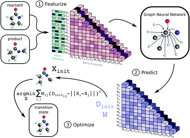
The workflow to generate transition state geometries involves several steps, which we roughly divide into featurization, prediction, and optimization. We first generate attributed graph structures of the reactant and product and effectively average them to create a graph structure representative of the TS. We feed this TS graph through a fully-connected graph neural network (GNN), which generates an updated graph representation of the TS.^76,77 An additional dense layer receives the updated TS graph and predicts values for two matrices necessary for a nonlinear least squares (NLS) optimization. The first matrix, D_init, is the network prediction of the TS distance matrix, which represents Euclidean distances between all pairs of atoms. The second matrix, W, is a set of weights used for the NLS optimization. Each entry in W corresponds to a pairwise distance in D_init and denotes the importance of each distance during reconstruction of the TS coordinates. The final coordinates of the TS, X, are the result of the NLS optimization, which minimizes the weighted residuals between D_init and pairwise distances in X. Once trained, our method generates initial guesses for isomerization TS structures within seconds. Fig. 1 highlights the key steps in the method, while the ESI† provides further details. Our code is available on GitHub at https://github.com/PattanaikL/ts_gen.

Fig. 1 Illustration of workflow used to generate TS structures. Given input 3D reactant and product structures, we generate an initial representation of the TS graph by calculating averaged atom and bond features. We feed this input to a GNN, which generates an updated representation of the TS graph. We then pass this updated representation through a dense layer to predict the TS distance matrix, D_init, and the NLS weight matrix, W. Finally, we perform an NLS optimization to recover the TS coordinates, X.

2.2 Dataset

We train the model on a recently published dataset of gas phase organic chemistry reactions.⁷⁸ These data were generated with the single-ended growing string method, so the reactions correspond to elementary steps through a single saddle point on the PES. All reactions involve anywhere from 3–7 heavy atoms including carbon, oxygen, and nitrogen (4–21 total atoms including hydrogens). We filter the data to reactions that contain a single product to include only isomerization reactions. Ref. 78 provides the data at two levels of DFT, but we limit our focus to the high level (ωB97X-D3 with a def2-TZVP basis set). Our final dataset consists of approximately 1000 unique reactants and 8500 reactions, which we divide randomly in an 80 : 10 : 10 split for training, validation, and testing.

2.3 Featurization

To train and test the model, we first transform individual log files from ref. 78 into structure-data files (SDFs) for the reactant, product, and TS. Our workflow uses reactant and product data to create an input attributed graph G with vertices (atoms), edges (bonds), and corresponding initial features for atoms and bonds. Note that since both the reactant and product contain the same number of atoms, it is straightforward to build G as an averaged representation for the TS. Importantly, the edge features include the exponential of the averaged distance between atoms i and j between the reactant and product along with whether or not a bond is broken or formed and if the bond is aromatic. The atom features only include the identity of the atom encoded numerically via atomic number and with a one-hot vector.

2.4 Prediction

The attributed 2D graph representation serves as the input to the GNN, which follows an update procedure for nodes and edges similar to ref. 77. First, we feed both the atom and bond features through dense layers to initialize the network. Next, the GNN iteratively updates the bond and atom features, and since this network is fully connected, it updates each edge and vertex with information from all other edges and vertices. After three iterations, we feed the final edge representation to another dense layer and symmetrize the output. The corresponding tensors represent the model's prediction of the TS distance matrix (D_init) and a weight matrix (W) for the forthcoming optimization. We detail the mathematical formalization of this network in the ESI.†

2.5 Optimization

We generate an initialization of the TS geometry (X_init in Fig. 1) for the NLS optimization in two steps using multidimensional scaling theory. First, we calculate the Gram matrix with the predicted D_init matrix. Then, we perform an eigendecomposition of the Gram matrix to calculate X_init by concatenating the eigenvectors corresponding to the three largest eigenvalues. To recover the final TS coordinates, we optimize this initialization with an NLS algorithm defined by the following:

The desired TS geometry is a result of minimizing the weighted residuals between D_init and pairwise distances in X. When training the network, we calculate network loss by first recalculating the distance matrix from X (which we denote as D) and computing the absolute difference between D and the ground truth distance matrix given by ref. 78. We backpropagate this loss through the coordinate recovery procedure and the GNN in an end-to-end manner. This way, we not only learn the TS distance matrix prediction (D_init), but we also learn to weight the distance prediction appropriately (W). The end-to-end differentiability of our network combined with its ability to both learn and weight the TS distance matrix prediction are the crucial aspects of our method that make it successful. The ESI† provides further details regarding the mathematics.

2.6 Verification

We employ a TS verification method similar to ref. 34. The automated quantum mechanics (QM) workflow first uses the TS geometry generated by the model as an initial guess in a TS optimization with the Berny method¹⁰ and verifies the presence of a first-order saddle point by checking for exactly one imaginary frequency. It then feeds the optimized transition state to two intrinsic reaction coordinate (IRC) calculations, which link the saddle point to its corresponding reactant and product PES minima by a mass-weighted downhill optimization.⁷⁹ Thus, we spawn forward and reverse IRCs on the optimized TS to generate the corresponding reactant and product, which we further verify with a stationary point optimization and frequency calculation, ensuring all frequencies are real. Our workflow feeds these generated reactant and product geometries to OpenBabel, which infers connectivity using its “connect-the-dots” method by adding bonds to atoms closer than their combined covalent radii while maintaining minimum distance and valence constraints.⁸⁰ We use these connections to compare graph connectivity between IRC reactants and products and original reactants and products. Matches between both sets for both molecules correspond to a successful TS generation.

3 Results and discussion

3.1 Model structures before QM optimization

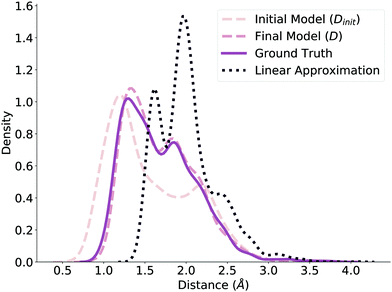
Before submitting the structures generated by the model to the verification workflow, we ensure that our method predicts valid geometries. That is, we evaluate whether the method in Fig. 1 independently produces realistic and realizable distance matrices. To check this, we plot the distribution of normalized distances generated by our model before and after the NLS optimization (D_init and D, respectively) and compare it to the ground truth distribution of normalized distances reported by ref. 78, shown in Fig. 2. The dashed lines correspond to the model predictions, while the solid line corresponds to the ground truth distribution. Note that we limit these distributions to the reaction core (i.e., bonds that changed during reaction) to further highlight differences. Even before optimization, the D_init distribution closely resembles the ground truth distribution; after optimization, the D and ground truth distributions are nearly identical, emphasizing the benefits of the NLS procedure. We additionally compare against a fourth distribution of distances generated by using the average distance between reactant and product, shown as the dotted line in Fig. 2. This distribution is significantly different from D_init, demonstrating that the GNN produces an effective initialization and further verifying that our model generates reasonable geometries to use as initial guesses.

Fig. 2 Initial model, final model, ground truth, and linear approximation distribution of distances between atoms of the reaction core of TS structures in the test set. The final model and ground truth distributions are nearly identical, while the linear approximation distribution is different.

3.2 Model importance weighting

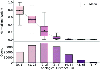
To understand why the model produces valid geometries, we investigate the weight matrices predicted by the model, which emphasize which bonds are considered important during reconstruction of the final TS guess geometry (step 3 in Fig. 1). We extract these weights from our network and normalize them by the maximum weight for each molecule. We then bin the weights based on the average topological distance between reactant and product (i.e., the average number of bonds separating the two atoms to which the weight corresponds), shown in Fig. 3, along with counts for each bin. As topological distance between atoms increases, the value of the weight assigned to this distance decreases. That is, the model prioritizes preserving distances of nearby atoms when reconstructing coordinates from the predicted distance matrix. Again, this reinforces that the model learns which distances are important and focuses on retaining these local distances during generation of the TS structure.

Fig. 3 Box plots of normalized weight matrices binned by average topological distance between reactant and product of test set reactions. Values of weights decrease as number of bonds between atoms increase.

3.3 Model performance on similar reactions

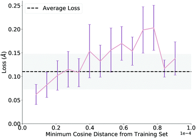
We evaluate overall performance on a held-out test set on which the model performs well, achieving an average test loss of 0.11 angstroms (average atomic difference in distance between model and ground truth structures per atom) before QM optimization. After investigating several trends, we report a noteworthy correlation, plotted in Fig. 4. To generate this plot, we extract learned embeddings of each reaction as the output of the GNN in both the training and test sets. We calculate pairwise cosine distances between each point in the two sets and plot the minimum cosine distance value for each test data point against its loss from the network. Thus, the plot claims that network loss increases as the similarity between the test data point and training data decreases. While we expect this trend, its proof allows us to add a pseudo-confidence metric to each new TS prediction: any new reaction (within the interpolation space of the training data) that is similar to data in the training set (as defined by a GNN embedding similarity less than a cutoff value of 0.3 × 10⁻⁴) should generally receive a reliable prediction from the network. The decreased loss above a cosine distance of 0.8 × 10⁻⁴ is likely an artifact of the few examples that have a high dissimilarity from the training set (n < 5 for each of the last two bins).

Fig. 4 Minimum cosine distance of test set from training set using learned embeddings from the GNN. Network loss increases as the distance between the test data point and training data increases. Each full bar corresponds to a single standard deviation, and the gray shading corresponds to a full standard deviation with respect to the average loss.

3.4 Correlation between difference success criteria

It is important to recognize the multiple success criteria we use to assess our results. While the deep learning method generates TS geometries based on difference in distances from the ground truth (network loss), our true measure of success is defined by the verification workflow. We employ this workflow on the test set of 834 reactions and achieve a 71% success rate, correctly following 595 initial guesses generated by our model to the ground truth reactants and products. Because the dataset contains a number of uncommon reactions, we check performance on the subset of reactions that match reaction families defined in the Reaction Mechanism Generator (RMG).³ On this set of well-known gas-phase reaction types, our model achieves a success rate of 89%. These success rates, while short of ideal production percentages, represent better success rates than traditional string and expert-guided methods.³¹ Furthermore, of the TS optimizations that succeeded, they required an average of only 20 Berny iterations to converge, showing the success of the algorithm at generating initial guess geometries.

We also assess the various failure modes: 41% of failures involve failed TS optimizations, 6% involve failed IRCs, 21% involve failed ground state optimizations, and the final 32% of failures are mismatches between the calculated ground state structures and the reported reactant and product structures. Of the TS optimization failures, 83% involve poor geometry failures (ex. exceeding the maximum number of steps allowed), 10% involve symmetry issues related to the generated internal coordinates, and 7% identify the incorrect number of imaginary frequencies. Clearly, a plurality of the failures involve inadequate initial guesses, motivating further optimization of our network.

We ensure the deep learning method is compatible with our true measure of success by plotting the loss distributions of the successes and failures as defined by the verification workflow, shown in Fig. 5. While the distributions are clearly different, the overlap suggests that the naïve network loss function (difference in distances) we use could be improved. We further comment on this issue after investigating specific examples.

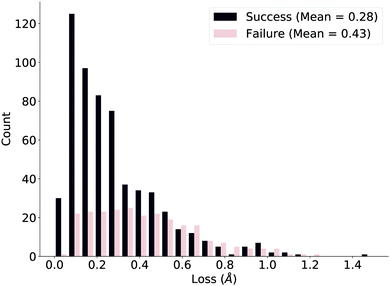Fig. 5 Loss distributions of successful and failed reactions in the test set as defined by the verification workflow. The distributions are markedly different but stress room for improvement.

3.5 Positive examples

Fig. 6 illustrates several examples of reactions fed to our model; each illustration positions the reactant and product at the beginning and end of the arrow, respectively, and indicates the ground truth TS with a blue highlight (left) and the model-generated TS with a green highlight (right). A.1 shows a simple 1,3-migration reaction, predicted correctly by the linear approximation method as well. Our network correctly predicts many similar simple reactions. A.2 shows a more complicated example, where the geometry of the migrating group changes during the transformation. While the linear approximation method does not correctly predict this TS structure, our method effectively learns the geometric changes necessary to generate this TS. Note that, while our method slightly rotates the oxygenated group, the guess geometry is adequate enough to converge to the saddle point structure with the subsequent Berny optimization. In other words, many of the guesses generated by our method are “close enough” to the target geometry to pass the subsequent verification workflow.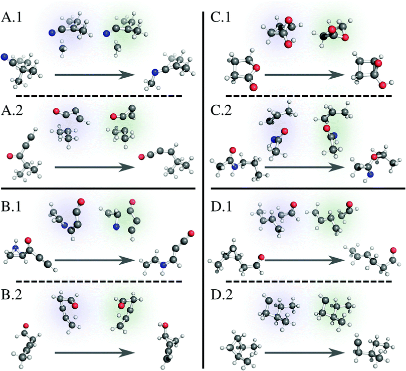

Fig. 6 Example reactions with reactant and product at the beginning and end of the arrow, respectively, showing the ground truth TS with a blue highlight (left) and the model-generated TS with a green highlight (right). (A.1) A simple reaction predicted correctly by the model. (A.2) A complicated reaction predicted correctly by the model. (B.1) A complex reaction predicted incorrectly by the model. (B.2) A TS where the model predicts a mirror image of the correct structure but fails the verification workflow. (C.1) and (C.2) TSs where the model predicts a mirror image of the correct structure, and the TSs pass the verification workflow. (D.1) A reaction with a deceptively large neural network loss that passes the verification workflow. (D.2) A reaction with a near zero neural network loss that surprisingly fails the verification workflow. We render all 3D structures with PyMol.⁸¹

3.6 Negative examples

Of the reactions that fail verification, many mirror example B.1. Here, several bonds break and form at once, as the linear oxocarbon group rearranges its connection to the aziridine group, which also simultaneously breaks apart. The model does not capture the orientation between the two groups well enough to pass a Berny optimization. Similar complicated reactions with large distance changes between reactant and product structures compose the failures (Fig. S3, ESI†). B.2 shows an example of a different but more significant failure mode. While the model TS structure correctly captures the transformation, it is nearly a mirror image of the reported transition state. Because we use the distance matrix to generate a TS structure, the target geometry is not entirely unique, and in a few cases, this fact results in a converged TS guess that contains one or more planes of symmetry with the ground truth geometry. Since our goal is to generate TS geometries to calculate rate constants, this is not a significant issue; a mirror image-converged TS produces the same numerical values for a rate constant. B.2, however, is an example where the mirror TS fails subsequent Berny optimization, which is problematic.

3.7 False positives

Examples C.1 and C.2 show similar TS structures generated by our model that are near mirror images of the reported ground truth but pass the verification workflow. Again, while this is not always an issue, we designate these examples as “false positives” and are actively working on modifications to relieve this issue. For database construction, we suggest using the IRC-optimized reactants and products.

3.8 False negatives

While investigating specific examples, we also discover failed structures we designated as “false negatives.” These examples are a direct result of our multiple criteria for success discussed earlier: loss as calculated by the network and success as defined by the verification workflow. Example D.1 shows a structure that registers a large loss value from the network but passes the verification workflow. In this example, the model TS methyl and aldehyde groups are rotated from the ground truth. While this difference in distances triggers a large loss, it is easily adjusted during subsequent optimization, further suggesting that using absolute difference of distances as a loss function for the network is a naïve option that should be improved. Conversely, D.2 shows a structure that registers a near-zero network loss but fails the verification workflow. Initial glance at the structure shows little difference between model and ground truth geometries, suggesting an unknown job error. We run each quantum calculation at a set of default parameters without further refinement for failed jobs; we are also implementing an automated strategy to restart failed jobs.

3.9 Limitations

The incapability of the current model to capture orientation constraints represents a significant limitation. Again, while this issue—which manifests itself with symmetric structures from the reported ground truth—does not usually affect any derived rate constants, it may affect generation of complex TS structures in the future, such as those for metal-catalyzed reactions with intricate ligand interactions or generally for enantioselective reactions. Traditional methods that use distance geometry to generate structures use orientation constraints defined for chiral atoms based on signed volumes. Structure optimization methods use these constraints as a part of the energy function, usually within a simulated annealing framework (that is, the orientation constraints are only used to refine the structure, not to generate an initial guess). Replicating such an approach is possible to alleviate the current model limitations, but the orientation constraints for a TS must be learned since they are not known a priori.

The model design also prevents TS generation for multi-reactant reactions. Such a model would need to orient multiple reactants together before using the current method to generate a TS structure; we leave this task for future models. For large structures with many TS conformations, this method should be paired with more developed theories which consider TS conformations. That is, upon finding a single TS structure, one must explore other low energy TS structures to accurately calculate kinetic rates. If the identity of the reactive species is different than the structure provided by the user, (e.g., for reactions with specific reactive protonation states or tautomers), the current algorithm will not find an appropriate TS. Finally, input reactions to the model must indicate the atom-mapping between reactants and products. While this is the case for most double-ended methods, it represents a barrier towards a fully-automated TS search algorithm. Fortunately, automated atom-mapping algorithms do exist and researchers continue to refine and improve them.^82–85

4 Conclusions

The availability of high-quality data and the recent prevalence of deep learning in the natural sciences have combined to usher in a new era of predictive chemistry. Computation especially offers a platform to both generate large quantities of data and extract trends generally applicable to out-of-domain samples. Here, we developed a deep learning model to generate three-dimensional transition state structures given the geometries of the reactant and product trained on a diverse dataset of gas-phase organic reactions. Our method produced viable geometries before QM optimization and achieved excellent results on an external test set via a rigorous verification workflow. We hope that users adopt our method to generate isomerization transition state structures relevant for their research and use our model as a basis for architectures involving even more complex chemical transformations.

Conflicts of interest

There are no conflicts to declare.

Acknowledgements

We gratefully acknowledge the Machine Learning for Pharmaceutical Discovery and Synthesis consortium for funding this work. We also thank Connor Coley for commenting on the manuscript.

References

1. M. R. Harper, K. M. Van Geem, S. P. Pyl, G. B. Marin and W. H. Green, Combust. Flame, 2011, 158, 16–41.
2. S. Gudiyella, Z. J. Buras, T.-C. Chu, I. Lengyel, S. Pannala and W. H. Green, Ind. Eng. Chem. Res., 2018, 57, 7404–7420.
3. C. W. Gao, J. W. Allen, W. H. Green and R. H. West, Comput. Phys. Commun., 2016, 203, 212–225.
4. A. J. Lawson, J. Swienty-Busch, T. Géoui and D. Evans, The Future of the History of Chemical Information, ACS Publications, 2014, pp. 127–148.
5. J. Mayfield, D. Lowe and R. Sayle, Abstracts of Papers of The American Chemical Society, 2017.
6. R. Straker, Q. Peng, A. Mekareeya, R. Paton and E. Anderson, Nat. Commun., 2016, 7, 1–9.
7. D. A. DiRocco, Y. Ji, E. C. Sherer, A. Klapars, M. Reibarkh, J. Dropinski, R. Mathew, P. Maligres, A. M. Hyde and J. Limanto, et al. , Science, 2017, 356, 426–430.
8. M. Orlandi, F. D. Toste and M. S. Sigman, Angew. Chem., 2017, 129, 14268–14272.
9. Y. Guan and S. E. Wheeler, Angew. Chem., Int. Ed., 2017, 56, 9101–9105.
10. H. B. Schlegel, J. Comput. Chem., 1982, 3, 214–218.
11. H. B. Schlegel, Theor. Chim. Acta, 1984, 66, 333–340.
12. C. Peng, P. Y. Ayala, H. B. Schlegel and M. J. Frisch, J. Comput. Chem., 1996, 17, 49–56.
13. J. Zheng and M. J. Frisch, J. Chem. Theory Comput., 2017, 13, 6424–6432.
14. T. A. Halgren and W. N. Lipscomb, Chem. Phys. Lett., 1977, 49, 225–232.
15. C. Peng and H. Bernhard Schlegel, Isr. J. Chem., 1993, 33, 449–454.
16. A. R. Rosales, T. R. Quinn, J. Wahlers, A. Tomberg, X. Zhang, P. Helquist, O. Wiest and P.-O. Norrby, Chem. Commun., 2018, 54, 8294–8311.
17. G. Henkelman, B. P. Uberuaga and H. Jónsson, J. Chem. Phys., 2000, 113, 9901–9904.
18. B. Peters, A. Heyden, A. T. Bell and A. Chakraborty, J. Chem. Phys., 2004, 120, 7877–7886.
19. A. Goodrow, A. T. Bell and M. Head-Gordon, J. Chem. Phys., 2008, 129, 174109.
20. P. Zimmerman, J. Chem. Theory Comput., 2013, 9, 3043–3050.
21. A. Behn, P. M. Zimmerman, A. T. Bell and M. Head-Gordon, J. Chem. Phys., 2011, 135, 224108.
22. S. Mallikarjun Sharada, P. M. Zimmerman, A. T. Bell and M. Head-Gordon, J. Chem. Theory Comput., 2012, 8, 5166–5174.
23. H. B. Schlegel, Theor. Chim. Acta, 1992, 83, 15–20.
24. K. K. Irikura and R. D. Johnson, J. Phys. Chem. A, 2000, 104, 2191–2194.
25. A. Laio and M. Parrinello, Proc. Natl. Acad. Sci. U. S. A., 2002, 99, 12562–12566.
26. L.-P. Wang, A. Titov, R. McGibbon, F. Liu, V. S. Pande and T. J. Martnez, Nat. Chem., 2014, 6, 1044.
27. M. Yang, J. Zou, G. Wang and S. Li, J. Phys. Chem. A, 2017, 121, 1351–1361.
28. S. Maeda, T. Taketsugu and K. Morokuma, J. Comput. Chem., 2014, 35, 166–173.
29. P. M. Zimmerman, J. Comput. Chem., 2013, 34, 1385–1392.
30. P. M. Zimmerman, J. Comput. Chem., 2015, 36, 601–611.
31. C. A. Grambow, A. Jamal, Y.-P. Li, W. H. Green, J. Zador and Y. V. Suleimanov, J. Am. Chem. Soc., 2018, 140, 1035–1048.
32. J. Zádor and H. N. Najm, KinBot 1.0: A code for automatic PES exploration., Sandia national lab.(snl-ca), livermore, ca (united states) technical report, 2013.
33. R. Van de Vijver and J. Zádor, Comput. Phys. Commun., 2020, 248, 106947.
34. P. L. Bhoorasingh and R. H. West, Phys. Chem. Chem. Phys., 2015, 17, 32173–32182.
35. P. L. Bhoorasingh, B. L. Slakman, F. Seyedzadeh Khanshan, J. Y. Cain and R. H. West, J. Phys. Chem. A, 2017, 121, 6896–6904.
36. D. G. Truhlar, B. C. Garrett and S. J. Klippenstein, J. Phys. Chem., 1996, 100, 12771–12800.
37. D. Sheppard, R. Terrell and G. Henkelman, J. Chem. Phys., 2008, 128, 134106.
38. G. N. Simm, A. C. Vaucher and M. Reiher, J. Phys. Chem. A, 2018, 123, 385–399.
39. J. P. Unsleber and M. Reiher, Annu. Rev. Phys. Chem., 2020, 71, 121–142.
40. M. H. Segler, M. Preuss and M. P. Waller, Nature, 2018, 555, 604–610.
41. C. W. Coley, W. H. Green and K. F. Jensen, Acc. Chem. Res., 2018, 51, 1281–1289.
42. P. Schwaller, R. Petraglia, V. Zullo, V. H. Nair, R. A. Haeuselmann, R. Pisoni, C. Bekas, A. Iuliano and T. Laino, arXiv preprint arXiv:1910.08036, 2019.
43. Q. Yang, V. Sresht, P. Bolgar, X. Hou, J. L. Klug-McLeod and C. R. Butler, et al. , Chem. Commun., 2019, 55, 12152–12155.
44. B. Chen, T. Shen, T. S. Jaakkola and R. Barzilay, arXiv preprint arXiv:1910.09688, 2019.
45. J. N. Wei, D. Duvenaud and A. Aspuru-Guzik, ACS Cent. Sci., 2016, 2, 725–732.
46. J. Bradshaw, M. J. Kusner, B. Paige, M. H. Segler and J. M. Hernández-Lobato, arXiv preprint arXiv:1805.10970, 2018.
47. D. Fooshee, A. Mood, E. Gutman, M. Tavakoli, G. Urban, F. Liu, N. Huynh, D. Van Vranken and P. Baldi, Mol. Syst. Des. Eng., 2018, 3, 442–452.
48. P. Schwaller, T. Laino, T. Gaudin, P. Bolgar, C. A. Hunter, C. Bekas and A. A. Lee, ACS Cent. Sci., 2019, 5, 1572–1583.
49. C. W. Coley, W. Jin, L. Rogers, T. F. Jamison, T. S. Jaakkola, W. H. Green, R. Barzilay and K. F. Jensen, Chem. Sci., 2019, 10, 370–377.
50. D. K. Duvenaud, D. Maclaurin, J. Iparraguirre, R. Bombarell, T. Hirzel, A. Aspuru-Guzik and R. P. Adams, Advances in neural information processing systems, 2015, pp. 2224–2232.
51. C. W. Coley, R. Barzilay, W. H. Green, T. S. Jaakkola and K. F. Jensen, J. Chem. Inf. Model., 2017, 57, 1757–1772.
52. K. Schutt, P. Kessel, M. Gastegger, K. Nicoli, A. Tkatchenko and K.-R. Muller, J. Chem. Theory Comput., 2018, 15, 448–455.
53. J. S. Smith, B. T. Nebgen, R. Zubatyuk, N. Lubbers, C. Devereux, K. Barros, S. Tretiak, O. Isayev and A. E. Roitberg, Nat. Commun., 2019, 10, 1–8.
54. K. Yang, K. Swanson, W. Jin, C. Coley, P. Eiden, H. Gao, A. Guzman-Perez, T. Hopper, B. Kelley and M. Mathea, et al. , J. Chem. Inf. Model., 2019, 59, 3370–3388.
55. C. A. Grambow, L. Pattanaik and W. H. Green, J. Phys. Chem. Lett., 2020, 11, 2992–2997.
56. J. You, B. Liu, Z. Ying, V. Pande and J. Leskovec, Advances in neural information processing systems, 2018, pp. 6410–6421.
57. Q. Liu, M. Allamanis, M. Brockschmidt and A. Gaunt, Advances in neural information processing systems, 2018, pp. 7795–7804.
58. M. H. Segler, T. Kogej, C. Tyrchan and M. P. Waller, ACS Cent. Sci., 2018, 4, 120–131.
59. R. Gómez-Bombarelli, J. N. Wei, D. Duvenaud, J. M. Hernández-Lobato, B. Sánchez-Lengeling, D. Sheberla, J. Aguilera-Iparraguirre, T. D. Hirzel, R. P. Adams and A. Aspuru-Guzik, ACS Cent. Sci., 2018, 4, 268–276.
60. W. Jin, R. Barzilay and T. Jaakkola, arXiv preprint, arXiv:1802.04364, 2018.
61. J. Bradshaw, B. Paige, M. J. Kusner, M. Segler and J. M. Hernández-Lobato, Advances in Neural Information Processing Systems, 2019, pp. 7935–7947.
62. W. Gao and C. W. Coley, J. Chem. Inf. Model., 2020 DOI:10.1021/acs.jcim.0c00174.
63. N. Anand and P. Huang, Advances in Neural Information Processing Systems, 2018, pp. 7494–7505.
64. M. AlQuraishi, Cell Syst., 2019, 8, 292–301.
65. J. Ingraham, A. Riesselman, C. Sander and D. Marks, International Conference on Learning Representations, 2019.
66. F. Noé, G. De Fabritiis and C. Clementi, Curr. Opin. Struct. Biol., 2020, 60, 77–84.
67. N. W. Gebauer, M. Gastegger and K. T. Schütt, arXiv preprint, arXiv:1810.11347, 2018.
68. M. Hoffmann and F. Noé, arXiv preprint, arXiv:1910.03131, 2019.
69. N. Gebauer, M. Gastegger and K. Schütt, Advances in Neural Information Processing Systems, 2019, pp. 7564–7576.
70. T. Lemke and C. Peter, J. Chem. Theory Comput., 2019, 15, 1209–1215.
71. G. N. Simm and J. M. Hernández-Lobato, arXiv preprint, arXiv:1909.11459, 2019.
72. J. Behler and M. Parrinello, Phys. Rev. Lett., 2007, 98, 146401.
73. S. Chmiela, H. E. Sauceda, K.-R. Müller and A. Tkatchenko, Nat. Commun., 2018, 9, 1–10.
74. H. E. Sauceda, S. Chmiela, I. Poltavsky, K.-R. Müller and A. Tkatchenko, arXiv preprint, arXiv:1909.08565, 2019.
75. N. Gerrits, K. Shakouri, J. Behler and G.-J. Kroes, J. Phys. Chem. Lett., 2019, 10, 1763–1768.
76. S. Kearnes, K. McCloskey, M. Berndl, V. Pande and P. Riley, J. Comput.-Aided Mol. Des., 2016, 30, 595–608.
77. P. W. Battaglia, J. B. Hamrick, V. Bapst, A. Sanchez-Gonzalez, V. Zambaldi, M. Malinowski, A. Tacchetti, D. Raposo, A. Santoro and R. Faulkner, et al., arXiv preprint, arXiv:1806.01261, 2018.
78. C. A. Grambow, L. Pattanaik and W. H. Green, Sci. Data, 2020, 7, 1–8.
79. K. Fukui, Acc. Chem. Res., 1981, 14, 363–368.
80. N. M. O’Boyle, M. Banck, C. A. James, C. Morley, T. Vandermeersch and G. R. Hutchison, J. Cheminf., 2011, 3, 33.
81. The PyMOL Molecular Graphics System, Version 2.3.2, Schrödinger, LLC.
82. D. Fooshee, A. Andronico and P. Baldi, J. Chem. Inf. Model., 2013, 53, 2812–2819.
83. N. Osório, P. Vilaça and M. Rocha, International Conference on Practical Applications of Computational Biology & Bioinformatics, 2017, pp. 257–264.
84. W. Jaworski, S. Szymkuć, B. Mikulak-Klucznik, K. Piecuch, T. Klucznik, M. Kaźmierowski, J. Rydzewski, A. Gambin and B. A. Grzybowski, Nat. Commun., 2019, 10, 1–11.
85. P. Schwaller, B. Hoover, J.-L. Reymond, H. Strobelt and T. Laino, ChemRxiv, 2020 DOI:10.26434/chemrxiv.12298559.v1.

---

Footnote

† Electronic supplementary information (ESI) available: Additional model, dataset, and training details. See DOI: 10.1039/d0cp04670a

---