
 Open Access Article
 This Open Access Article is licensed under a
 Creative Commons Attribution 3.0 Unported Licence
Quantum simulation of conical intersections
Yuchen
Wang
 and
David A.
Mazziotti
*
and
David A.
Mazziotti
*
Department of Chemistry and The James Franck Institute, The University of Chicago, Chicago, Illinois 60637, USA. E-mail: damazz@uchicago.edu
First published on 8th April 2024
Abstract
We explore the simulation of conical intersections (CIs) on quantum devices, setting the groundwork for potential applications in nonadiabatic quantum dynamics within molecular systems. The intersecting potential energy surfaces of H3+ are computed from a variance-based contracted quantum eigensolver. We show how the CIs can be correctly described on quantum devices using wavefunctions generated by the anti-Hermitian contracted Schrödinger equation ansatz, which is a unitary transformation of wavefunctions that preserves the topography of CIs. A hybrid quantum-classical procedure is used to locate the seam of CIs. Additionally, we discuss the quantum implementation of the adiabatic to diabatic transformation and its relation to the geometric phase effect. Results on noisy intermediate-scale quantum devices showcase the potential of quantum computers in dealing with problems in nonadiabatic chemistry.
1 Introduction
Nonadiabatic processes involve nuclear motion on multiple potential energy surfaces (PESs). These processes are ubiquitous in nature and have been studied extensively in diverse areas such as spectroscopy, solar energy conversion, chemiluminescence, photosynthesis, and photostability of biomolecules.1–17 Different potential energy surfaces can intersect at regions that exhibit a conical-shaped topography, known as conical intersections (CIs).18–21 In the vicinity of CIs, the Born–Oppenheimer approximation which assumes adiabaticity breaks down. Systems with nonadiabaticity can undergo sudden changes in their dominant configurations at CIs, leading to the classical and well-known “hop” picture between different electronic states.22 CIs act as highly efficient channels for converting external excitation energy, usually carried by a photon, to internal electronic energy. Their characterization is crucial to understand rich photochemistry and photobiology processes involving energy conversion.CIs are in general difficult to treat with quantum mechanical methods for several reasons. First, from the perspective of electronic structure theory, the excited states are harder to compute than the ground state as they correspond to first-order critical points rather than the global minimum. Moreover, the nonunitary ansatz for the wavefunction employed in some methods, such as standard coupled cluster (CC) methods, gives an incorrect topography of CIs.23–26 Second, since most electronic structure programs work under the Born–Oppenheimer approximation, results obtained from these programs are not readily applicable for subsequent chemical dynamics studies, especially near CIs. The process of converting the original adiabatic electronic structure data to a diabatic representation, referred as diabatization, is an active yet non-unified field due to the non-uniqueness of quasi-diabatic representations.27–41 Third, the dynamics of nonadiabatic systems typically require a more complex treatment than the dynamics on a single potential energy surface. For example, we need to expand wavefunctions in the basis of every diabatic state to account for effective state transition in quantum dynamics.1
Quantum computers could be a natural solution for nonadiabatic chemistry.42–50 To address some of the concerns in the last paragraph, we observe first that the gate operations are unitary, which makes it convenient to implement a unitary ansatz of wavefunctions (e.g., the unitary coupled cluster (UCC) ansatz51,52 or the anti-Hermitian contracted Schrödinger equation (ACSE) ansatz53–61). They offer robust and accurate solutions to the electronic structure data near CIs. In fact, for the ACSE ansatz used in this paper, classical calculations of CIs are well established.62–65 Second, quantum computers are ideal tools to perform unitary and even nonunitary propagation66,67 with a possible polynomial scaling advantage over classical computers where the coupling potential term can be expressed as an entanglement of encoded qubits.42 Third, the transformation from adiabatic wavefunctions to diabatic wavefunctions is unitary and can be easily implemented as parametric gates during state preparation on quantum computers. The geometric phase,45,46,68,69 a global phase factor dressing the wavefunctions near CIs, can also be encoded with simple rotations in the Pauli basis, which is a natural advantage of quantum computers.
In this paper we evaluate the performance of quantum computers in describing CIs. Some key issues associated with CIs, such as seam curvature, optimization and geometric phase are discussed. We implement the electronic structure simulation of H3+ with and without noise using the excited-state contracted quantum eigensolver (CQE) proposed in ref. 70 in which the wavefunctions are generated by the ACSE ansatz. The theory and methodology of CI including an overview of CQE are presented in Section 2. Results and outlooks are further discussed in Sections 3 and 4, respectively.
2 Theory
2.1 Diabatic Hamiltonian matrix and CIs
We start from the adiabatic electronic Schrödinger equation,| (Ĥa(r;R) − EJ)|ΨaJ(r;R)〉 = 0 | (1) |
Here, r and R denote the electronic and nuclear coordinates and J is a state index. The semicolon indicates that the Hamiltonian is parametrically dependent upon nuclear coordinates arising from the separation of electronic and nuclear degrees of freedom. This approximation, however, fails to describe nonadiabatic dynamics because in the vicinity of conical intersection, different adiabatic wavefunctions produce almost degenerate energies and result in singular derivative coupling vectors, defined below
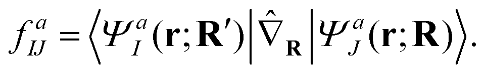 | (2) |
Under such circumstances it is often necessary to invoke the diabatic representation that produces well-described and smooth state couplings and wavefunctions.36 The diabatic representation is related to adiabatic representation through a unitary transformation of wavefunction,
| |Ψd(r;R)〉 = U(r;R)|Ψa(r;R)〉. | (3) |
If U is chosen such that fdIJ = 0 everywhere, then we consider the representation strictly diabatic. However, it has been proven that a strict diabatic representation does not exist for polyatomic molecules; hence, we refer to these states as “quasi-diabatic,” and the condition for vanishing derivative couplings in the diabatic representation becomes a condition for minimizing ||fdIJ||.27
The electronic Schrödinger equation can then be rewritten in the diabatic form as
| [Hd(R) − IEJ(R)]dJ(R) = 0 | (4) |
| (H11 − H22)2 + 4H12H21 = 0 | (5) |
When wavefunctions are generated from non-Hermitian techniques such as standard coupled cluster methods, the above equation is the only constraint to form CIs. However, this creates a nonphysical (N − 1) artifact that accompanies complex eigenvalues in the vicinity of true CIs, where N is the molecular degree of freedom.23–26 The true CI is a submanifold of the potential energy surfaces where the following two constraint equations, one for diagonal and one for off-diagonal term,
| H11 = H22, H12 = H21 = 0 | (6) |
It is then easily recognized that the dimension of CIs is (N − 2). While the diagonal condition is easy to constrain, the off-diagonal condition is subtle because it is not directly available in electronic structure programs. For some molecules, as we will show in this paper, it is possible to find two states with high symmetry such that the couplings between them are strictly zero by symmetry, a situation known as symmetry-required CIs. The symmetry, however, does not serve as a necessary condition for the existence of CIs as some CIs occur in the more general category of “accidental” CIs.19
2.2 Geometric phase effect
Most modern quantum chemistry programs assume the Born–Oppenheimer approximation and thus, produce electronic structure data in the adiabatic representation. Given the limitations of the adiabatic representation in nonadiabatic chemistry, there has been significant research effort directed towards determining the transformation from the adiabatic representation to the diabatic representation. The reason for the abundance of such diabatization techniques is that quasi-diabatic states are not unique.27 For two-state diabatization, some literature expresses the unitary in eqn (3) as a rotation matrix parameterized by the angle θ,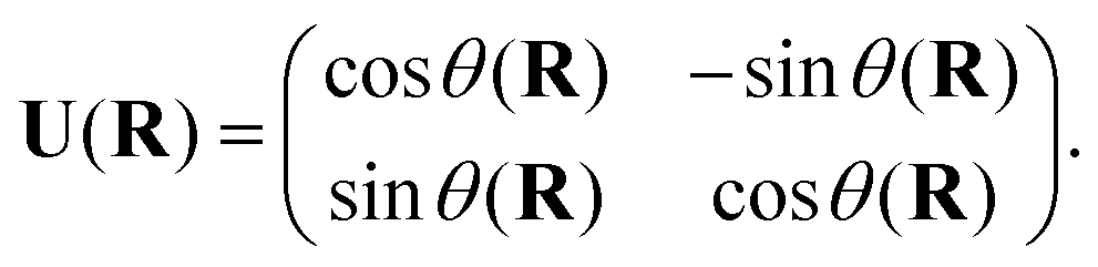 | (7) |
We remind the reader that the expression might naturally lead to the assumption that θ is a continuous function of R, but this is not necessarily true in the presence of CIs due to the geometric phase effect. The geometric phase effect requires that wavefunctions that are transported around a path enclosing a CI acquire an additional phase factor.68,71,72 A geometry-dependent and state-dependent factor eiAK(R)(K = I,J) must be included in the adiabatic wavefunction. The natural advantage of using qubits to represent this two-state diabatization is that both are isomorphic to the special unitary group of degree 2. Indeed on quantum computers, the phase factor can be implemented as a simple rotation gate parametrized by AK(R). One of the authors has shown in previous work73 that AJ(R) can be evaluated from the integral below,
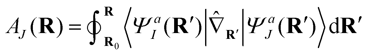 | (8) |
2.3 Variance-based contracted quantum eigensolver
The electronic structure calculation in this work is performed with a variance-based contracted quantum eigensolver (CQE) that has been proposed in a previous paper.70 The algorithm is briefly reviewed here.The variance (denoted as Var) of the system is defined as:
| Var[Ψm[2Fm]] = 〈Ψm|(Ĥ − Em)2|Ψm〉 | (9) |
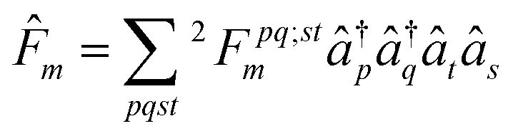
We minimize the variance with respect to the parametric two-body anti-Hermitian operator ![[F with combining circumflex]](https://www.rsc.org/images/entities/i_char_0046_0302.gif) m, where the wavefunction from ACSE theory at the mth iteration is given by the unitary ansatz as
m, where the wavefunction from ACSE theory at the mth iteration is given by the unitary ansatz as
| |Ψm〉 = em|Ψm−1〉 | (10) |
 | (11) |
m: | (12) |
![[capital Gamma, Greek, circumflex]](https://www.rsc.org/images/entities/i_char_e132.gif) pqst = â†pâ†qâtâs and the equation
pqst = â†pâ†qâtâs and the equation| 2Dpqst = 〈Ψm|pqst|Ψm〉. | (13) |
We provide additional comments regarding why variance-based CQE is suitable to describe the CIs. The convergence depends on the choice of the initial guess, which can be generated from single Slater determinant or a linear combination of them. It will converge to the nearest minimum of the variance without knowledge of the lower states. Here by nearest, we mean the most similar in configuration composition. This state-specific feature can be beneficial in studying the CIs. It allows us to tackle a specific state during the slow variation of molecular geometry without concern that the adiabatic states will cross. Note this also coincides with the idea of configurational-uniformity-based diabatization as first proposed by Nakamura and Truhlar.29
3 Results
We demonstrate the approach to computing the CI with the molecule H3+. The relative positions of the three co-planar hydrogen atoms are described in polar coordinates as (R,0), (R,π) and (ρ,θ) where R ≥ 0, ρ ≥ 0, 0 ≤ θ < 2π, allowing us to represent the molecular geometry by the set of coordinates (R,ρ,θ). Distances are given in the atomic unit bohr unless specified otherwise. Calculations are performed with the IBM Quantum statevector simulator and FakeLagosV2 backend. The statevector simulation is performed without noise, while the fake backend mimics the noise behavior of the real IBM quantum computer Lagos. The quantum simulation result is benchmarked with full configuration interaction calculations. All computations are performed in the minimal Slater-type orbital (STO-3G) basis set. The one- and two-electron integrals are obtained with Maple Quantum Chemistry Package.74,75 Here and below we denote full configuration interaction as FCI to distinguish it from the abbreviation for the conical intersection (CI).3.1 Electronic structure of H3+
The H3+ molecule exhibits arguably the simplest CI. Nonetheless, despite its simplicity, the molecule is an important species in astrochemistry, providing a useful benchmark for the study of CIs.76–83 We compute the first three states of H3+ with Sz = 0. A compact mapping is used to reduce the number of required qubits to three for the first and second excited states (denoted as E1 and E2) of H3+. The mapping is described here. We denote the configuration state function as |ij〉, (1 ≤ i,j ≤ 3) with the Sz = +1/2 electron occupying the ith molecular orbital and the Sz = −1/2 electron occupying the jth molecular orbital. The dimension of FCI matrix is 9. A further reduction is performed by eliminating |11〉 by observing that it has almost no coupling to the E1 and E2 states. Although |11〉 can couple to other higher states and in principle affect the diagonalization result, the truncation has negligible effect on the energy of E1 and E2 (<10−8 Hartree), resulting in a total qubit number of log2![[thin space (1/6-em)]](https://www.rsc.org/images/entities/char_2009.gif) 8 = 3.
8 = 3.
We analyze the electronic structure property of H3+ using the highly-symmetric D3h point group. The first and second excited states correspond to the two components of an E′ irreducible representation and thus form the symmetry-required CIs. We plot the potential energy curve in Fig. 1 obtained from the statevector simulator and a fake-backend simulator. A zoomed region of the degeneracy is given in the figure as well. The two excited states always overlap in the FCI scheme, which is consistent with our electronic structure knowledge of the system. On a noiseless statevector simulator we achieve an energy accuracy of 10−6 Hartree, where the only error comes from the trotterization, proving the exactness of the ACSE ansatz. After introducing device noise, the error for each individual state is around 12 mhartree. It is worth noting that since the error is quite uniform for both states, the error of their energy gap is significantly smaller, which is quite promising for predicting the energetic degeneracy.
 | ||
Fig. 1 Potential energy curve calculated by FCI as well as noiseless and noise simulators. Molecule is treated in the D3h symmetry, where the polar coordinates of the three hydrogen atoms are (R,0), (R,π) and  . Note that E1 and E2 are degenerate in FCI result due to symmetry. . Note that E1 and E2 are degenerate in FCI result due to symmetry. | ||
We next plot the dissociation curve at a lower symmetry, namely C2v in Fig. 2. The discontinuity of the E2 curve is due to crossings with intruder states. We are particularly interested in the CIs between E1 and E2, where the two states coincide at a D3h geometry. Despite the relatively large error of individual states, the prediction of the location of the CIs is surprisingly accurate (<0.01 bohr). As mentioned before, if the error induced by noise is nearly uniform for both states and for all geometries, then the effect of noise is only to shift both potential energy surfaces by a similar amount, which should not significantly affect the topography of the CIs. To verify this, in Fig. 3 we plot the coupled potential energy surfaces as a function of the coordinates of the third hydrogen atom. It can be seen that the topography of the CIs is well reproduced. The expected cusps induced by random noise are barely discernible due to the uniformity of noise. We note, however, that although the potential energy surfaces and relative energy gap are well reproduced, the absolute error still remains challenging on noise intermediate-scale quantum (NISQ) devices and further error mitigation techniques are needed.
 | ||
| Fig. 2 Potential energy curve calculated by FCI and the noise simulator. Molecule is treated in the C2v symmetry, where the polar coordinates of the three hydrogen atoms are (1,0), (1,π) and (R,π/2). | ||
 | ||
| Fig. 3 Intersecting adiabatic potential energy surfaces calculated from variance CQE. The grid size is 20 × 12. Additional points are placed in the vicinity of the CI. For better illustration, we use Cartesian coordinate with the coordinates of the three atoms being (−1,0,0), (1,0,0) and (x,y,0). Unit is bohr. | ||
3.2 Locating the seam of CI
The search of the minimum energy CI (MEX) is done by minimizing the constrained Lagrangian proposed in previous works,84,85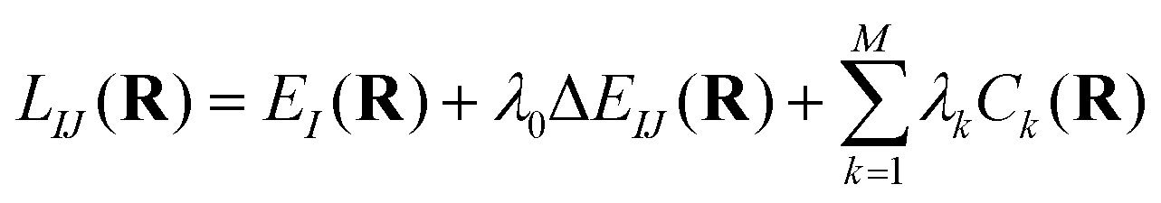 | (14) |
In a previous paper, we showed that the gradient of Lagrangian corresponding to the geometry parameter set R can be obtained with classical calculations.85 Here we use a hybrid method, where single-point energy calculations are performed with the variance-based CQE and the energy gradient is obtained by performing calculations at different geometries and then taking finite differences with a stepsize of 0.1.
The dimension of CI for the triatomic molecule is only one. By varying one molecular coordinate and fixing the rest, we should obtain a one-dimensional curve that corresponds to the seam of the CI. For the special case between the E1 and E2 of H3+, we know that this curve is unique and corresponds to the D3h geometries in Fig. 1. We report the optimization results by setting R to 2.0 bohr and optimizing over the position of the third hydrogen (r,θ). We use a gradient-like Newton–Raphson method with fixed step size of 0.1 where the Hessian of the Lagrangian is approximated by the identity matrix.
A typical optimization process is shown in Fig. 4 by plotting the trajectory of the third unfixed hydrogen atom along the iterations. The geometry parameter and energy difference are reported in Table 1. The performance is quite robust despite the simple setup, suggesting the gradient from quantum devices is resilient enough for geometry optimization purposes. The energy difference decreases during the optimization, except in the first iteration. This exception can occur because the Lagrangian includes contributions beyond the energy difference. An important observation is that, the noise on NISQ simulators introduces a small oscillation around our targeted D3h CI. The errors in the bond distance and bond angle, however, are quite small, which helps to demonstrate the accuracy of our description of the CIs.
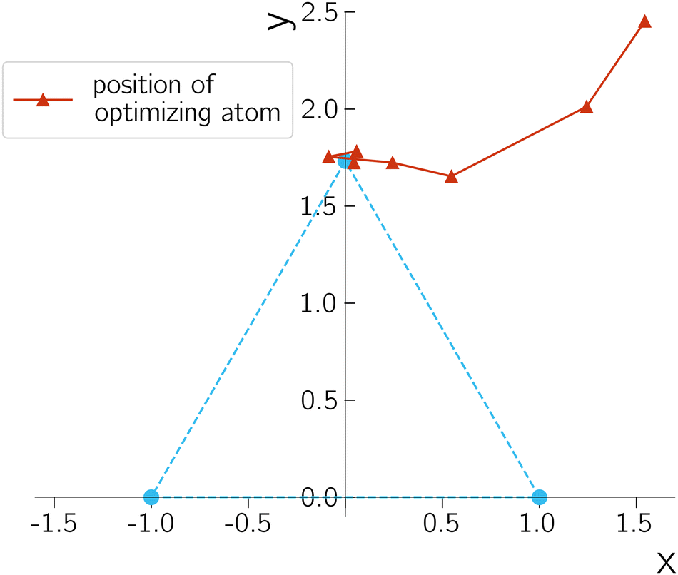 | ||
| Fig. 4 Trajectory of the unfixed hydrogen atom during optimization. The desired D3h geometry is indicated with blue dots. Cartesian coordinate is used for plotting with the coordinates of the two fixed hydrogen atoms being (−1,0,0), (1,0,0) and the optimizing one being (x,y,0). Unit is bohr. | ||
| Iteration number | θ (°) | ρ (bohr) | ΔE (Hartree) |
|---|---|---|---|
| 0 | 57.819 | 2.897 | 0.044 |
| 1 | 58.293 | 2.364 | 0.066 |
| 2 | 71.721 | 1.741 | 0.063 |
| 3 | 81.977 | 1.741 | 0.032 |
| 4 | 92.807 | 1.756 | 0.014 |
| 5 | 88.136 | 1.783 | 0.009 |
| 6 | 88.537 | 1.724 | 0.005 |
| Exact | 90 | 1.732 | 0 |
4 Conclusions and outlook
Current state-of-art nonadiabatic quantum dynamics are limited to small molecules due to their exponential scaling with respect to the active vibrational modes. Quantum computers may potentially provide a solution. In the future quantum devices with hundreds of qubits may be able to perform nonadiabatic quantum dynamics simulations that are either too expensive or intractable on high-performance classical computers. This paper provides a foundation for simulating the CIs on quantum computers, paving the way for advancements in quantum-based simulations for nonadiabatic molecular systems. Using a variance-based CQE, the energies of intersecting potential energy surfaces of molecular H3+ are accurately computed. The study achieves a correct representation of CI topography through a wavefunction generated by a unitary ansatz from ACSE theory. Future work includes realizing diabatization and quantum dynamics of complex nonadiabatic molecular system on quantum devices.Conflicts of interest
The authors declare no competing financial interest.Acknowledgements
Y. W. acknowledges helpful discussion with Dr Yafu Guan and Prof. David R. Yarkony. D. A. M. gratefully acknowledges the Department of Energy, Office of Basic Energy Sciences Grant DE-SC0019215, the U.S. National Science Foundation Grant CHE-2155082, and the U.S. National Science Foundation Grant RAISE-QAC-QSA, Grant DMR-2037783. We acknowledge the use of IBM Quantum services for this work. The views expressed are those of the authors and do not reflect the official policy or position of IBM or the IBM Quantum team.Notes and references
- H. Guo and D. R. Yarkony, Phys. Chem. Chem. Phys., 2016, 18, 26335–26352 RSC.
- B. J. Schwartz, E. R. Bittner, O. V. Prezhdo and P. J. Rossky, J. Chem. Phys., 1996, 104, 5942–5955 CrossRef CAS.
- B. G. Levine and T. J. Martnez, Annu. Rev. Phys. Chem., 2007, 58, 613–634 CrossRef CAS PubMed.
- P. V. Demekhin and L. S. Cederbaum, J. Chem. Phys., 2013, 139, 154314 CrossRef PubMed.
- J. E. Subotnik, A. Jain, B. Landry, A. Petit, W. Ouyang and N. Bellonzi, Annu. Rev. Phys. Chem., 2016, 67, 387–417 CrossRef CAS PubMed.
- T. E. Li, B. Cui, J. E. Subotnik and A. Nitzan, Annu. Rev. Phys. Chem., 2022, 73, 43–71 CrossRef CAS PubMed.
- B. F. Curchod and T. J. Martnez, Chem. Rev., 2018, 118, 3305 CrossRef CAS PubMed.
- S. Matsika, J. Phys. Chem. A, 2004, 108, 7584–7590 CrossRef CAS.
- S. Matsika and P. Krause, Annu. Rev. Phys. Chem., 2011, 62, 621 CrossRef CAS PubMed.
- Q. L. Nguyen, V. A. Spata and S. Matsika, Phys. Chem. Chem. Phys., 2016, 18, 20189–20198 RSC.
- M. S. Schuurman and A. Stolow, Annu. Rev. Phys. Chem., 2018, 69, 427 CrossRef CAS PubMed.
- Y. Guan, C. Xie, D. R. Yarkony and H. Guo, Phys. Chem. Chem. Phys., 2021, 23, 24962–24983 RSC.
- Y. Wang, H. Guo and D. R. Yarkony, Phys. Chem. Chem. Phys., 2022, 24, 15060–15067 RSC.
- J.-G. Zhou, Y. Shu, Y. Wang, J. Leszczynski and O. Prezhdo, J. Phys. Chem. Lett., 2024, 15, 1846–1855 CrossRef CAS PubMed.
- M. Baer, Phys. Rep., 2002, 358, 75–142 CrossRef CAS.
- B. Mukherjee, K. Naskar, S. Mukherjee, S. Ghosh, T. Sahoo and S. Adhikari, Int. Rev. Phys. Chem., 2019, 38, 287–341 Search PubMed.
- K. Naskar, S. Mukherjee, B. Mukherjee, S. Ravi, S. Mukherjee, S. Sardar and S. Adhikari, J. Chem. Theory Comput., 2020, 16, 1666–1680 CrossRef CAS PubMed.
- H. Köuppel, W. Domcke and L. Cederbaum, Adv. Chem. Phys., 1984, 59–246 CrossRef.
- D. R. Yarkony, Rev. Mod. Phys., 1996, 68, 985 CrossRef CAS.
- W. Domcke, D. Yarkony and H. Köppel, Conical intersections: Electronic structure, dynamics & spectroscopy, World Scientific, 2004, vol. 15 Search PubMed.
- W. Domcke and D. R. Yarkony, Annu. Rev. Phys. Chem., 2012, 63, 325 CrossRef CAS PubMed.
- J. C. Tully, J. Chem. Phys., 1990, 93, 1061 CrossRef CAS.
- A. Köhn and A. Tajti, J. Chem. Phys., 2007, 127, 044105 CrossRef PubMed.
- S. Gozem, F. Melaccio, A. Valentini, M. Filatov, M. Huix-Rotllant, N. Ferre, L. M. Frutos, C. Angeli, A. I. Krylov and A. A. Granovsky, et al. , J. Chem. Theory Comput., 2014, 10, 3074 CrossRef CAS PubMed.
- S. Faraji, S. Matsika and A. I. Krylov, J. Chem. Phys., 2018, 148, 044103 CrossRef PubMed.
- S. Thomas, F. Hampe, S. Stopkowicz and J. Gauss, Mol. Phys., 2021, 119, e1968056 CrossRef.
- C. A. Mead and D. G. Truhlar, J. Chem. Phys., 1982, 77, 6090 CrossRef CAS.
- K. Ruedenberg and G. J. Atchity, J. Chem. Phys., 1993, 99, 3799 CrossRef CAS.
- H. Nakamura and D. G. Truhlar, J. Chem. Phys., 2001, 115, 10353 CrossRef CAS.
- W. Eisfeld and A. Viel, J. Chem. Phys., 2005, 122, 204317 CrossRef PubMed.
- D. Opalka and W. Domcke, J. Chem. Phys., 2013, 138, 224103 CrossRef PubMed.
- T. Lenzen and U. Manthe, J. Chem. Phys., 2017, 147, 084105 CrossRef PubMed.
- R. J. Cave and M. D. Newton, Chem. Phys. Lett., 1996, 249, 15 CrossRef CAS.
- A. J. Dobbyn and P. J. Knowles, Mol. Phys., 1997, 91, 1107 CAS.
- C. R. Evenhuis and M. A. Collins, J. Chem. Phys., 2004, 121, 2515–2527 CrossRef CAS PubMed.
- D. R. Yarkony, C. Xie, X. Zhu, Y. Wang, C. L. Malbon and H. Guo, Comput. Theor. Chem., 2019, 1152, 41 CrossRef CAS.
- Y. Wang, Y. Guan and D. R. Yarkony, J. Phys. Chem. A, 2019, 123, 9874 CrossRef CAS PubMed.
- S. Han, Y. Wang, Y. Guan, D. R. Yarkony and H. Guo, J. Chem. Theory Comput., 2020, 16, 6776 CrossRef CAS PubMed.
- C. Li, S. Hou and C. Xie, J. Chem. Theory Comput., 2023, 19, 3063 CrossRef CAS PubMed.
- J. Wang, F. An, J. Chen, X. Hu, H. Guo and D. Xie, J. Chem. Theory Comput., 2023, 19, 2929 CrossRef CAS PubMed.
- E. Vandaele, M. Mališ and S. Luber, J. Chem. Theory Comput., 2024, 20, 856–872 CrossRef CAS PubMed.
- P. J. Ollitrault, G. Mazzola and I. Tavernelli, Phys. Rev. Lett., 2020, 125, 260511 CrossRef CAS PubMed.
- P. J. Ollitrault, A. Miessen and I. Tavernelli, Acc. Chem. Res., 2021, 54, 4229–4238 CrossRef CAS PubMed.
- J. Whitlow, Z. Jia, Y. Wang, C. Fang, J. Kim and K. R. Brown, Nat. Chem., 2023, 1–6 Search PubMed.
- C. H. Valahu, V. C. Olaya-Agudelo, R. J. MacDonell, T. Navickas, A. D. Rao, M. J. Millican, J. B. Pérez-Sánchez, J. Yuen-Zhou, M. J. Biercuk, C. Hempel, T. R. Tan and I. Kassal, Nat. Chem., 2023, 15, 1503–1508 CrossRef CAS PubMed.
- C. S. Wang, N. E. Frattini, B. J. Chapman, S. Puri, S. M. Girvin, M. H. Devoret and R. J. Schoelkopf, Phys. Rev. X, 2023, 13, 011008 CAS.
- S. Yalouz, B. Senjean, J. Günther, F. Buda, T. E. OBrien and L. Visscher, Quantum Sci. Technol., 2021, 6, 024004 CrossRef.
- S. Yalouz, E. Koridon, B. Senjean, B. Lasorne, F. Buda and L. Visscher, J. Chem. Theory Comput., 2022, 18, 776–794 CrossRef CAS PubMed.
- K. Omiya, Y. O. Nakagawa, S. Koh, W. Mizukami, Q. Gao and T. Kobayashi, J. Chem. Theory Comput., 2022, 18, 741–748 CrossRef CAS PubMed.
- S. Zhao, D. Tang, X. Xiao, R. Wang, Q. Sun, Z. Chen, X. Cai, Z. Li, H. Yu and W.-H. Fang, 2024, arXiv:2402.12708.
- A. Anand, P. Schleich, S. Alperin-Lea, P. W. Jensen, S. Sim, M. Daz-Tinoco, J. S. Kottmann, M. Degroote, A. F. Izmaylov and A. Aspuru-Guzik, Chem. Soc. Rev., 2022, 51, 1659 RSC.
- J. Lee, W. J. Huggins, M. Head-Gordon and K. B. Whaley, J. Chem. Theory Comput., 2018, 15, 311 CrossRef PubMed.
- D. A. Mazziotti, Phys. Rev. Lett., 2006, 97, 143002 CrossRef PubMed.
- D. A. Mazziotti, Phys. Rev. A, 2007, 75, 022505 CrossRef.
- D. A. Mazziotti, Phys. Rev. A: At., Mol., Opt. Phys., 2007, 76, 052502 CrossRef.
- S. E. Smart and D. A. Mazziotti, Phys. Rev. Lett., 2021, 126, 070504 CrossRef CAS PubMed.
- S. E. Smart and D. A. Mazziotti, J. Chem. Theory Comput., 2022, 18, 5286–5296 CrossRef CAS PubMed.
- J.-N. Boyn and D. A. Mazziotti, J. Chem. Phys., 2021, 154, 134103 CrossRef CAS PubMed.
- J.-N. Boyn, A. O. Lykhin, S. E. Smart, L. Gagliardi and D. A. Mazziotti, J. Chem. Phys., 2021, 155, 244106 CrossRef CAS PubMed.
- S. E. Smart, J.-N. Boyn and D. A. Mazziotti, Phys. Rev. A, 2022, 105, 022405 CrossRef CAS.
- Y. Wang, L. M. Sager-Smith and D. A. Mazziotti, New J. Phys., 2023, 25, 103005 CrossRef.
- J. W. Snyder, A. E. Rothman, J. J. Foley and D. A. Mazziotti, J. Chem. Phys., 2010, 132, 154109 CrossRef PubMed.
- J. W. Snyder and D. A. Mazziotti, J. Chem. Phys., 2011, 135, 024107 CrossRef PubMed.
- J. W. Snyder and D. A. Mazziotti, J. Phys. Chem. A, 2011, 115, 14120–14126 CrossRef CAS PubMed.
- J. W. Snyder and D. A. Mazziotti, Phys. Chem. Chem. Phys., 2011, 14, 1660–1667 RSC.
- A. W. Schlimgen, K. Head-Marsden, L. M. Sager, P. Narang and D. A. Mazziotti, Phys. Rev. Lett., 2021, 127, 270503 CrossRef CAS PubMed.
- Z. Hu, R. Xia and S. Kais, Sci. Rep., 2020, 10, 3301 CrossRef CAS PubMed.
- H. C. Longuet-Higgins, U. Öpik, M. H. L. Pryce and R. Sack, Proc. R. Soc. London, Ser. A, 1958, 244, 1–16 CAS.
- E. Koridon, J. Fraxanet, A. Dauphin, L. Visscher, T. E. O'Brien and S. Polla, Quantum, 2024, 8, 1259 CrossRef.
- Y. Wang and D. A. Mazziotti, Phys. Rev. A, 2023, 022814 CrossRef CAS.
- C. A. Mead, Rev. Mod. Phys., 1992, 64, 51 CrossRef CAS.
- C. Xie, C. L. Malbon, H. Guo and D. R. Yarkony, Acc. Chem. Res., 2019, 52, 501–509 CrossRef CAS PubMed.
- Y. Wang and D. R. Yarkony, J. Chem. Phys., 2021, 155, 174115 CrossRef CAS PubMed.
- Maple, (Maplesoft, Waterloo, 2023).
- RDMChem, Quantum Chemistry Package (Maplesoft, Waterloo, 2023).
- H. Kamisaka, W. Bian, K. Nobusada and H. Nakamura, J. Chem. Phys., 2002, 116, 654 CrossRef CAS.
- L. P. Viegas, A. Alijah and A. J. Varandas, J. Chem. Phys., 2007, 126, 074309 CrossRef PubMed.
- P. Barragán, L. Errea, A. Macas, L. Méndez, I. Rabadán and A. Riera, J. Chem. Phys., 2006, 124, 184303 CrossRef PubMed.
- S. Mukherjee, D. Mukhopadhyay and S. Adhikari, J. Chem. Phys., 2014, 141, 204306 CrossRef PubMed.
- S. Ghosh, S. Mukherjee, B. Mukherjee, S. Mandal, R. Sharma, P. Chaudhury and S. Adhikari, J. Chem. Phys., 2017, 147, 074105 CrossRef PubMed.
- Z. Yin, B. J. Braams, B. Fu and D. H. Zhang, J. Chem. Theory Comput., 2021, 17, 1678 CrossRef CAS PubMed.
- Y. Guan, D. R. Yarkony and D. H. Zhang, J. Chem. Phys., 2022, 157, 014110 CrossRef CAS PubMed.
- S. Kwon, S. Sandhu, M. Shaik, J. Stamm, J. Sandhu, R. Das, C. V. Hetherington, B. G. Levine and M. Dantus, J. Phys. Chem. A, 2023, 127, 8633–8638 CrossRef CAS PubMed.
- M. R. Manaa and D. R. Yarkony, J. Chem. Phys., 1993, 99, 5251–5256 CrossRef CAS.
- Y. Wang and D. R. Yarkony, J. Chem. Phys., 2018, 149, 154108 CrossRef PubMed.
| This journal is © the Owner Societies 2024 |