
 Open Access Article
 This Open Access Article is licensed under a Creative Commons Attribution-Non Commercial 3.0 Unported Licence
Surface tension models for binary aqueous solutions: a review and intercomparison†
Judith
Kleinheins
 *a,
Nadia
Shardt‡
a,
Manuella
El Haber
b,
Corinne
Ferronato
b,
Barbara
Nozière
c,
Thomas
Peter
a and
Claudia
Marcolli
a
*a,
Nadia
Shardt‡
a,
Manuella
El Haber
b,
Corinne
Ferronato
b,
Barbara
Nozière
c,
Thomas
Peter
a and
Claudia
Marcolli
a
aInstitute for Atmospheric and Climate Science, ETH Zürich, Universitätstrasse 16, 8092 Zürich, Switzerland. E-mail: judith.kleinheins@env.ethz.ch
bIrcelyon, CNRS and Universite Lyon 1, Villeurbanne, France
cRoyal Institute of Technology (KTH), Department of Chemistry, Stockholm, Sweden
First published on 23rd March 2023
Abstract
The liquid–air surface tension of aqueous solutions is a fundamental quantity in multi-phase thermodynamics and fluid dynamics and thus relevant in many scientific and engineering fields. Various models have been proposed for its quantitative description. This Perspective gives an overview of the most popular models and their ability to reproduce experimental data of ten binary aqueous solutions of electrolytes and organic molecules chosen to be representative of different solute types. In addition, we propose a new model which reproduces sigmoidal curve shapes (Sigmoid model) to empirically fit experimental surface tension data. The surface tension of weakly surface-active substances is well reproduced by all models. In contrast, only few models successfully model the surface tension of aqueous solutions with strongly surface-active substances. For substances with a solubility limit, usually no experimental data is available for the surface tension of supersaturated solutions and the pure liquid solute. We discuss ways in which these can be estimated and emphasize the need for further research. The newly developed Sigmoid model best reproduces the surface tension of all tested solutions and can be recommended as a model for a broad range of binary mixtures and over the entire concentration range.
1. Introduction
The surface tension of aqueous solutions is a key physical property in many fields, influencing e.g. the efficiency of distillation trays,1 the biological functioning of lung surfactants,2 the size distribution of aerosol produced by medical nebulizers,3 and the number of aerosol particles activated to cloud droplets in the atmosphere.4 It depends on the type and concentration of the solutes, temperature, and the curvature of the surface, the latter becoming relevant only in droplets with radii of curvature approaching the molecular scale.5 Various techniques allow to measure the surface tension of large drops or bulk solutions. Instruments are also emerging to measure the surface tension of small droplets, such as atomic force microscopy6 and holographic optical tweezers.7 Most measurements of the surface tension of aqueous solutions reported in the literature, however, are bulk measurements and restricted to aqueous solutions with one solute only (binary solutions). Data of aqueous solutions with more than one solute (multi-component solutions) are scarce. Mathematical models of surface tension have been developed for different purposes, be it simply to convert discrete measurement data points into an analytical expression, or to predict the surface tension for unknown systems. The approach and the complexity of surface tension models in the literature varies widely, from models based on molecular dynamics,8–10 machine learning models,11–14 to empirical and thermodynamic models, each type of model being justified by its ability to fulfill a specific goal (e.g., accuracy, simplicity, or robustness). Given the importance of surface tension across various disciplines, it is important to develop mathematical tools that can accurately describe how surface tension varies as a function of solution composition.In many models for bulk aqueous solutions, surface tension is expressed as a function of composition at a constant temperature, using the surface tension of the pure components as input parameters. They differ with respect to their physical basis and derivation, their number of fitting parameters, and their ability to fit differently-shaped surface tension curves as a function of solute concentration. Some are mathematically equivalent, although having been derived in different ways. Moreover, some can be more easily extended to multi-component solutions than others. Often, a certain model is favoured for particular substances or in a specific field, such as liquid metal alloys, which is the major application area for the Butler equation,15 while atmospheric sciences rely often on the Szyszkowski–Langmuir model for the description of surface tension of liquid aerosol particles at high relative humidity.16–42 However, a systematic, interdisciplinary comparison of the performance of these models is lacking. In this study, we fill this gap by analyzing the performance of common surface tension models for bulk binary aqueous solutions.
The effect a solute has on the surface tension of water varies greatly with the type of solute. Electrolytes are known to increase the surface tension of the solution. Other substances, such as simple alcohols, have a lower pure component surface tension than water and thus lower the surface tension of the solution, with a more or less pronounced deviation from a linear mixing rule. Substances with a strong tendency to partition to the surface drastically lower the surface tension of a solution even when they are present in only very small amounts. The term “surfactants”, which stands for surface–active–agents, usually refers to this latter kind of substance (strong tendency to partition), while those substances with a weaker tendency to partition can be named “weak surfactants”.
In this study, we investigate whether a model can be found to apply to all of these solute types, as such a model would have several advantages: First, describing all substances with a single model allows a compressed representation of experimental data, requiring only fit parameters to be reported. Second, if the parameters of this model have physical meaning, the substances can be compared to each other by comparison of their parameters (e.g., their extent to which they partition to the surface). Lastly, such a model has the potential to be extended to a multi-component model for mixtures of different types of surface active species. Since experimental data for multi-component solutions are scarce, but experimental data for binary solutions are broadly available, a predictive model for multi-component solutions could be developed that is based on fitting to binary experimental data. In atmospheric sciences, electrolytes, weakly surface active organics and strong surfactants can be mixed together in one aerosol particle. Therefore, the ability of the binary model to fit all these substance types individually is a prerequisite for a model to predict the surface tension of the mixture.
In aiming for a universal surface tension model, a challenge is posed by substances whose pure liquid surface tension values are unknown because they crystallize in bulk volumes at the temperature where the surface tension is required (e.g. electrolytes). Small droplets containing such substances can easily supersaturate and remain liquid at concentrations where larger volumes would crystallize. Hence, for such systems a model is required that can predict surface tension at concentrations where measured values are lacking. Here, we test the ability of the models to predict the surface tension of crystallizing substances, and discuss different approaches to deal with these substances.
In the following, we first summarize the theoretical background of the most common surface tension models for aqueous bulk solutions and analyze their mathematical form. Second, we analyze the applicability and performance of comparable surface tension models on a set of ten test substances. In our results and discussion, we report difficulties and constraints of the different models, the best fit parameters for the tested substances as well as knowledge gaps suggesting needs for further research.
2. Overview of literature surface tension models
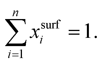
In the literature, various semi-empirical surface tension models for aqueous solutions can be found. Here, we summarize the main assumptions behind popular models, some characteristics of their equations and examples of their applications. A summary of these models is given in Table 1. All models are a function of either the mole fraction xi, the activity ai, or the molarity ci of the solute i, with| xi + xw = 1, | (1) |
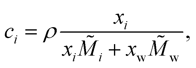 | (2) |
![[M with combining tilde]](https://www.rsc.org/images/entities/i_char_004d_0303.gif) i and w are the molar mass of the solute and of water, respectively. In this study, we define ai = γi·xi for organic substances, where γi is the activity coefficient of the solute, and ai = γi·mi for electrolytes, where mi is the molality of the solute. In principle, the enrichment of solute in the surface leads to its depletion in the bulk phase and therefore, the composition of the bulk phase xbulki needs to be distinguished from the total composition xtotali. This effect, however, only becomes relevant in small volumes, where the number of solute molecules at the surface Nsurfi accounts for a non-negligible fraction of the total number of solute molecules Ntotali. In large volumes, due to the lower surface-to-volume ratio, Nsurfi ≪ Ntotali ≈ Nbulki. In the following, therefore, we simply define xi := xbulki ≈ xtotali.
i and w are the molar mass of the solute and of water, respectively. In this study, we define ai = γi·xi for organic substances, where γi is the activity coefficient of the solute, and ai = γi·mi for electrolytes, where mi is the molality of the solute. In principle, the enrichment of solute in the surface leads to its depletion in the bulk phase and therefore, the composition of the bulk phase xbulki needs to be distinguished from the total composition xtotali. This effect, however, only becomes relevant in small volumes, where the number of solute molecules at the surface Nsurfi accounts for a non-negligible fraction of the total number of solute molecules Ntotali. In large volumes, due to the lower surface-to-volume ratio, Nsurfi ≪ Ntotali ≈ Nbulki. In the following, therefore, we simply define xi := xbulki ≈ xtotali.
| Name | Ref. | Equation for binary mixtures | Fit parameters | Multi-component solutions | Used in |
|---|---|---|---|---|---|
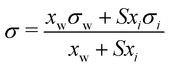
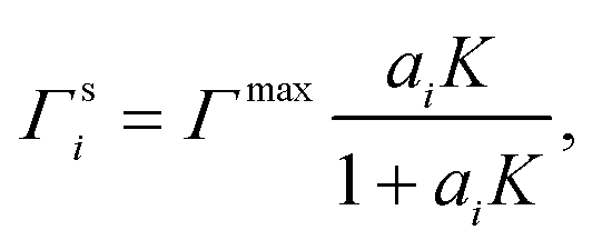
| Li & Lu model* | 43 |
|
Γ max, K | Two equations proposed43 | 44–46 |
| Szyszkowski–Langmuir equation | 47 and 48 | σ = σw − RTα·ln(1 +ci/β) | α, β | See21,25,27,49 | 16–42 |
| Statistical model* | 50–52 |
|
r, K, C | See Boyer et al.53 | 54 |
| Butler equation* | 55–59 |
|
— | Inherent | 44,45 and 60–64 |
| Tamura model* | 59 and 65 | σ 1/4 = ψsurfwσ1/4w + (1 − ψsurfw)σ1/4i | — | Not inherent | 44 and 45 |
| Eberhart model* | 66 |
|
S | Not inherent | 44 and 45 |
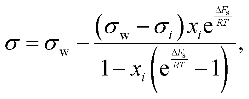
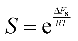
| Shereshefsky model | 67 |
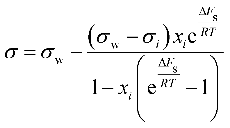
|
ΔFs | Not inherent | 68 |
| Connors–Wright model* | 69 |
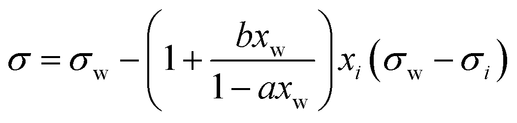
|
a, b | See Shardt et al.70 | 68 and 70 |
| Chunxi model | 71 |
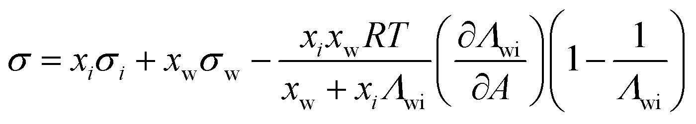
|
|
See Chunxi et al.71 | 32,72 and 73 |
2.1 Gibbsian surface tension models
Gibbs's work on the thermodynamics of surfaces in 1876 was a milestone in the science of surfaces and set the basis for many surface tension models thereafter. For bulk systems, the main idea in Gibbsian surface tension models is the concept of the Gibbs dividing surface—a theoretical phase of zero thickness, lying between the bulk phase and the gas phase. While for a real surface, the concentration of a substance follows a certain profile across the surface, in the Gibbs approach, this concentration profile is modelled by a step function, and the amount of substance that is under or over accounted by this approach is compensated for in the Gibbs dividing surface (surface excess).74–76 Different approaches exist about where to place the Gibbs dividing surface. Commonly, it is defined as the equimolar surface with respect to water, i.e. where the surface excess of water equals zero. Another approach defines the Gibbs dividing surface as the special equimolar surface where the sum of the surface excesses of all substances weighted by their molar volume equals zero, which is equivalent to setting the volume of the surface phase to zero.75 The location of the Gibbs dividing surface does not affect the magnitude of the surface tension for bulk systems, but it plays a role for liquid volumes of finite size, i.e. for small droplets with a diameter <10 nm.75Another fundamental ingredient for Gibbsian surface tension models is the Gibbs adsorption equation, which relates the composition of the surface to the surface tension. It is usually written as
 | (3) |
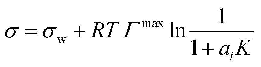
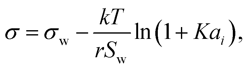
To relate the surface composition to the bulk composition, a Langmuir adsorption isotherm is often used. Langmuir adsorption was originally derived for the adsorption of an adsorbent from the gas phase to a solid substrate. It assumes (i) that the adsorbent behaves like an ideal gas with a certain partial pressure, (ii) that the adsorption rate K equals the desorption rate in equilibrium and (iii) that the solid substrate has a maximum number of binding sites Γmax.77 Analogously, to model the partitioning of a solute i from a liquid bulk phase to a liquid–gas interface, the partial pressure is replaced by the activity of the solute in the bulk ai, leading to:
 | (4) |
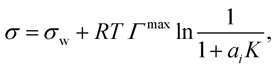 | (5) |
Sorjamaa et al.75 proposed a similar model consisting of a set of equations to calculate the surface tension of binary and multi-component solutions with the following differences from the Li & Lu model: (i) the Gibbs dividing surface is placed at the “special equimolar surface”, (ii) the activity coefficients of the solutes are calculated from Henrys law constants, and (iii) ideality is assumed for water.
Lastly, a famous model following the Gibbs–Langmuir approach is known as the Szyszkowski–Langmuir equation, sometimes also called “Szyszkowski equation of state”24 or “Szyszkowski–Langmuir adsorption isotherm”.16 Originally formulated as an entirely empirical model by Szyszkowski47 based on experiments with aqueous solutions containing fatty acids, this model was later interpreted thermodynamically by Langmuir.48 It can be written as
| σ = σw − RTα·ln(1 +ci/β), | (6) |
2.2 Statistical mechanics model
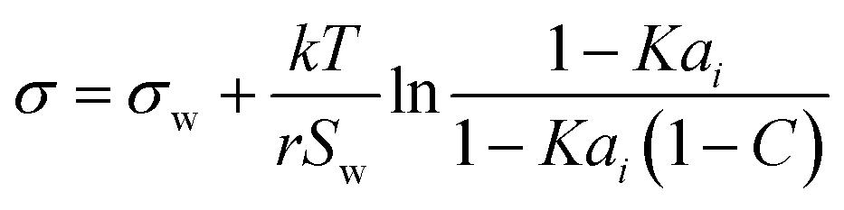
Aiming for a model that works equally well for non-electrolyte and electrolyte solutes over the full range of concentrations, Wexler and Dutcher50 derived a surface tension model from a Gibbs free energy expression using statistical mechanics (Statistical model). The sorption of solute molecules to the liquid–vapor interface is modelled by representing the surface as a monolayer and the bulk as a multilayer. The model is formulated for binary aqueous mixtures as | (7) |
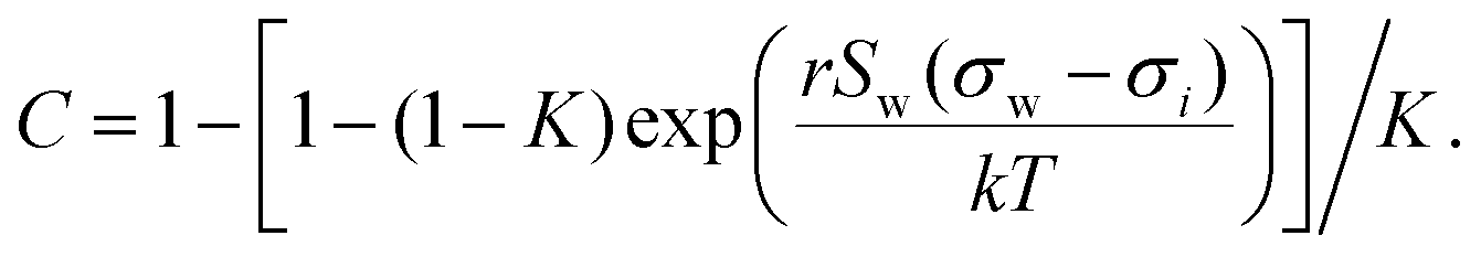 | (8) |
 | (9) |
In Boyer51 the predictive capabilities of the model were further improved by relating the model parameters to solute molecular properties, thereby reducing the number of free parameters. To this end, a number of alcohols, polyols and electrolytes have been tested. For the electrolytes, the root mean squared error (RMSE) of the fully predictive surface tension model is between 0.4 and 3.6 mN m−1. For the organics, a one-parameter version of the model leads to equally good RMSE values between 0.3 and 3.5 mN m−1. Results from their fully predictive model for alcohols are only shown for methanol, 1,2-ethanediol and 1,3-butanediol. For these three alcohols, their predictive model provides excellent agreement with the models that have one or two fitted parameters.
Boyer and Dutcher78 extended the single-solute model to a multiple-solute version, in order to model the surface tension of aqueous organic acid solutions including partial dissociation of the acid. For the seven di- and tricarboxylic acids that were examined, this “ternary model” shows a very similar fitting capability as the one-parameter-model neglecting dissociation (“binary model”), with differences in the RMSE of the models <0.02 mN m−1. This suggests that the inclusion of the dissociation of the acids does not improve the model considerably; however, the ternary model laid a foundation for the development of a general model for multi-component solutions as followed up by Boyer et al.53 Miles et al.54 have applied the multi-component model to picoliter NaCl–glutaric acid–water solution droplets of varying composition reaching good agreement with surface tension measurements obtained using a microdroplet dispenser and a holographic optical tweezer. A summary of all these model developments can be found in Boyer and Dutcher.52
Recently, Liu and Dutcher79 extended the surface tension model from Wexler and Dutcher50 to considering multiple surface layers to model the concentration depth profile at the surface. They compared model fits to experimental data for several organic and inorganic substances with good agreement, but the results are not compared to the simpler model version with a monolayer assumption for the surface. Thus it remains unclear if the higher complexity of the model actually leads to improved surface tension predictions.
In all mentioned publications from this research group, activity coefficients were calculated with their own activity coefficients model, which is based on the statistical mechanics of multilayer sorption.80–82
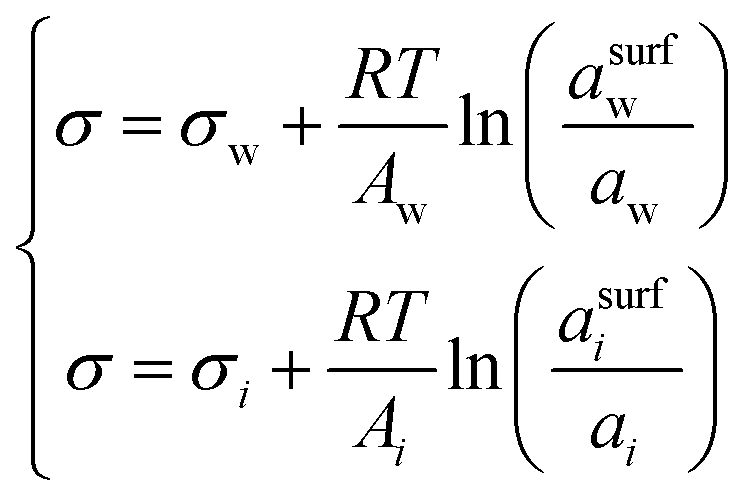
2.3 The Butler equation
In 1932, Butler,55 derived a set of equations to calculate the surface tension of bulk mixtures of any number of substances, which is commonly written as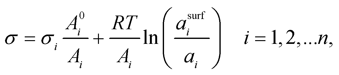 | (10) |
 | (11) |
| Ai = 1.021 × 10⁸V6/15cV4/15b, | (12) |
| Ai = V2/3iN1/3A, | (13) |
The Butler equation has been used for a variety of compounds, including liquid metal alloys,85,86 electrolyte solutions60,61 and atmospherically-relevant mixtures. Cai and Griffin62 calculated the surface tension of secondary organic aerosol particles applying the procedure described by Poling et al.59 This calculation was carried out in the context of evaluating for which compositions and particle sizes of secondary organic aerosol particles the Kelvin effect has to be considered for the gas–liquid partitioning of semi-volatile substances in aerosol chamber experiments. A comparison of the modelled surface tension values to experimental data was not done by Cai and Griffin,62 due to lack of experimental data.
In contrast, Topping et al.44 and Booth et al.45 systematically evaluated the performance of the predictive Butler equation (referred to as the model by Sprow & Prausnitz or Suarez) by comparing to experimental data for various single and multiple solute mixtures of atmospherically-relevant organic and inorganic compounds. They pointed out that for many atmospherically-relevant compounds σi is unknown, since the pure compounds tend to crystallize in the bulk at atmospheric conditions, hence making surface tension measurements in the bulk impossible. Therefore, they applied models to estimate σi, which resulted in poor performance compared to a surface tension model with fit parameters such as the Li & Lu model.
Werner et al.63,64 applied a Butler equation-based method of Li et al.60 to aqueous succinic acid solutions with64 and without63 inorganic salts and compared their results to experiments. Here, the original system of equations was reduced to one equation only, namely that for water. Further, they assumed, that msurfsuccinicacid = g·mbulksuccinicacid where m is the molality and g is the surface enrichment factor, the latter of which they obtained from X-ray photoelectron spectroscopy measurements and from molecular dynamics simulations. The modelled surface tensions could reproduce the trend of the measurements. It was also shown that inorganic salts further increase the surface enrichment of succinic acid.
2.4 Parachor model
A semi-empirical model for the surface tension of a single organic solute in water was described by Tamura et al.65 (Tamura model). It is based on the Macleod–Sugden correlation, which relates σi to liquid and vapor densities via a temperature independent parameter called the “parachor”. The final model equation is:59| σ1/4 = ψsurfwσ1/4w + (1 − ψsurfw)σ1/4i, | (14) |
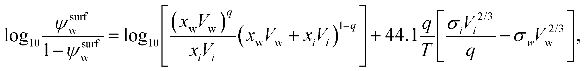 | (15) |
Topping et al.44 and Booth et al.45 tested the Tamura model as a fully predictive model for aqueous solutions of various organic and inorganic substances and a number of aqueous multi-component solutions. Since the Tamura model has no version for multi-component solutions, an additive approach was used for these, such that the deviations from σw caused by the individual solutes are simply added to give the total deviation of σ. The comparison to experimental data revealed large discrepancies of the model predictions, mostly due to the high uncertainty in σi values.
2.5 Simple thermodynamic models
Based on the assumption that the surface tension of a binary liquid mixture is an average of the pure substance surface tensions weighted by the surface concentrations, Eberhart66 derived a simple equation for the mixture surface tension, which for a single-solute–water mixture reads as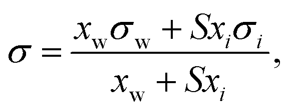 | (16) |
 | (17) |
 .
.
A simple model with two free parameters was derived by Connors and Wright69 (Connors–Wright model), based on the same assumption of σ being an average weighted by xsurfi but with additional assumptions about the state of the surface layer and by applying a Langmuir adsorption isotherm to describe the partitioning between bulk and the surface. For a single-solute–water mixture, it is written as
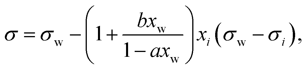 | (18) |
 | (19) |
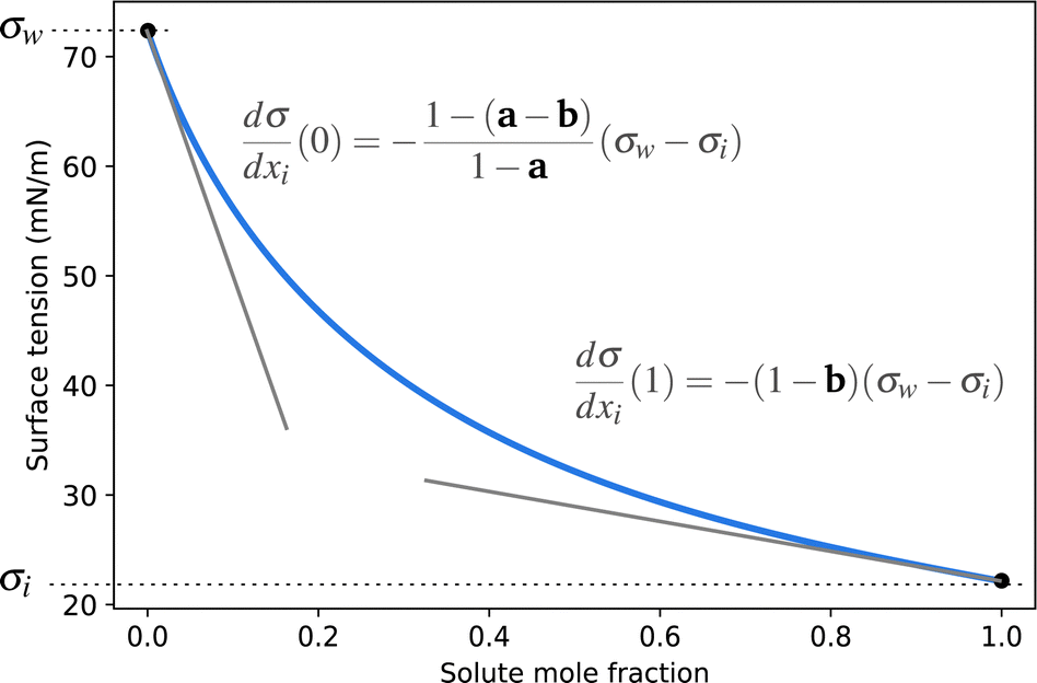 | ||
| Fig. 1 Illustration of the Connors–Wright function (blue solid line) and the influence of the parameters a and b on its slopes. | ||
Another two-parameter model was derived by Chunxi et al.71 (Chunxi model) based on the Wilson equation87 as
 | (20) |
Shardt and Elliott68 extended the Shereshefsky, Chunxi (referred to as Li et al.) and the Connors–Wright model to predict σ as a function of composition and temperature and compared their performance for 15 organic substances in a temperature range from 293 to 323 K. Overall, the Connors–Wright and the Chunxi model performed slightly better than the Shereshefsky model because of their additional fit parameter. Shardt and Elliott68 recommend to use the Connors–Wright model, since the parameters in the Chunxi model are temperature–dependent while the ones in the Connors–Wright model are not. Shardt et al.70 further extended the Connors–Wright model to multi-component solutions and nonaqueous systems that may contain a supercritical component.
In the field of atmospheric sciences, Hyvarinen et al.72 applied the Chunxi model for aqueous solutions of several dicarboxylic acids and cis-pinonic acid. The model was fitted to their own surface tension data at varying composition and temperature. The surface tensions of the supercooled pure acids were estimated with the method of MacLeod–Sugden and their temperature dependence was fitted to a linear equation. Vanhanen et al.73 applied the multi-component version of the Chunxi model to ternary solutions of NaCl, succinic acid and water. Finally, Prisle et al.32 fitted the Chunxi model to experimental σ data of sodium laurate solutions in a sensitivity study to predict the surface partitioning of fatty acid sodium salts during cloud droplet activation.
3. Methodology of model comparison
In order to assess the performance of surface tension models proposed in the literature, we compared their ability to fit experimental surface tension data. All models were tested with the same set of test substances, irrespective of their original purpose. To evaluate the surface tension model performance independently of the choice of activity coefficient models, we used the same activity coefficient model for all models and all substances. Experimental data as well as modelling was focused on ambient temperature in this study (20 °C < T < 25 °C). Note that models with temperature independent fit parameters allow the application of the fit parameters to any temperature, since the temperature dependence can be represented by σw(T) and σi(T), as shown by Shardt and Elliott68 for the Connors–Wright model. Therefore, many findings of this study should be valid at other temperatures, too. All models were fitted with the curve_fit() function in the module optimize of the Python package SciPy.883.1 Tested models
We evaluated the performance of the models marked with an asterisk in Table 1 as well as one additional model proposed by us (see below). To provide a level playing field, only models were selected that are a function of solute mole fraction or solute activity in the bulk and thus applicable to the entire concentration range. Therefore, the Szyszkowski–Langmuir equation was not analyzed, being only valid for dilute solutions as outlined above. We preferred the Eberhart model over the mathematically equivalent Shereshefsky model, since its fit parameters are dimensionless and therefore temperature independent. For the same reason, we preferred the Connors–Wright model over the Chunxi model. This leaves us with seven models to be tested. Also, all models were expressed in a form to be a direct function of σw and σi. This implied the reformulation of some models, as described in the following.The Li & Lu model was tested in two versions: the original model using ai (non-ideal) and a simplified version, where ideality is assumed by replacing ai with xi (ideal). Although the Li & Lu model is not a direct function of σi, a value for σi can be derived by examining the model at xi = 1 and replacing the parameter K:
 | (21) |
The Statistical model exists in different versions with zero to three fit parameters. Fully predictive or 1-parameter versions were developed only for alcohols and electrolytes so far and thus will not be examined here. The simplified version for very small K and high C values (eqn (9)), which applies to surface tension lowering substances (surfactants) is equivalent to the Li & Lu model and is thus covered by this model. Hence, in the following, with “Statistical model” we refer to the full model (eqn (7)). For a better comparison to the other models, here too, we rewrite the model as a function of σi, by replacing the parameter C (eqn (8)). Thus, if σi is known, the Statistical model has the two fit parameters r and K. The original model, based on its derivation, only allows K within [0,1]. In this study, however, we found that for surfactants, restricting K within [0,1] leads to fits very similar to the Li & Lu model, while allowing K to be negative improved the fits. This is clearly an unphysical usage of the original Statistical model turning it into a mixing rule that lacks thermodynamic background. Due to its improved performance we nevertheless include it in this study and label it Statistical unconstrained or abbreviated Stat. uncon. in the following. We also test the Statistical unconstrained model in an ideal and a non-ideal version.
To reduce the number of tested model versions, we performed a preliminary comparison between three versions of the Butler equation:
• Calculating Ai with eqn (12) (Goldsack and White84)
• Calculating Ai with eqn (13) (Sprow and Prausnitz56)
• Making Ai a fit parameter.
In agreement with Suarez et al.,57 fitting Ai turned out to be clearly superior to the fully predictive models (see Section 4 in ESI†). Therefore, we selected this option for the model comparison of the Butler equation in an ideal and a non-ideal version.
In the Tamura model, the parameter q represents the number of segments in a solute molecule, e.g. the carbon number for fatty acids, and should be limited to whole numbers. Tamura et al.65 suggest values for q for certain substances, but not for all substances that we intend to model and hence, we use it as a fit parameter. We also allow non-integer numbers for q here, due to better fit performance. The molar volumes of the solutes were calculated as Vi = /ρi with the molecular weight and the subcooled liquid density ρi. For organics, ρi was calculated using UManSysProp89 (method: Girolami, critical properties method: Nannoolal), and for NaCl, ρi = 2.09 g cm−3 was used.90 The molar volume of water was set to Vw = 18 cm3 mol−1.
The Eberhart model and the Connors–Wright model were used as shown in eqn (16) and (18), respectively.
Inspired by the “S”-shape of the surface tension curves on the logarithmic x-axis scale, we proposed a parametrized sigmoid function (Sigmoid model) in addition to the other models. We used the logistic function as a basis:
 | (22) |
 | (23) |
 | (24) |
 | (25) |
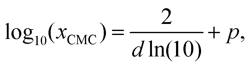 | (26) |
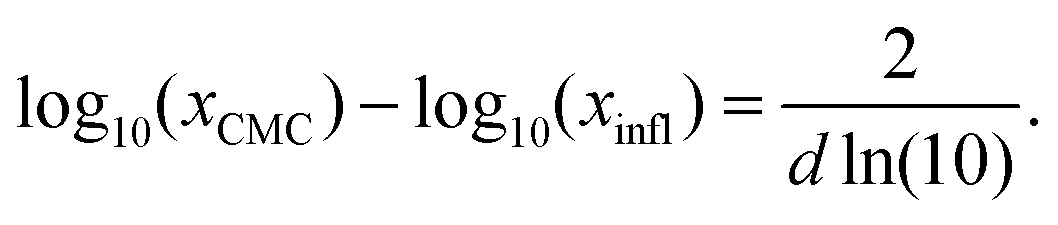 | (27) |
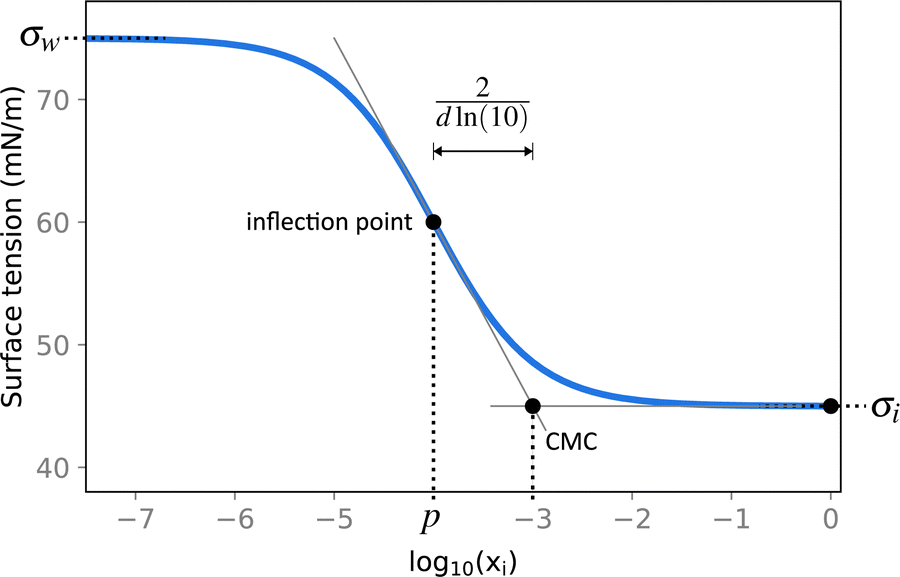 | ||
| Fig. 2 Illustration of the Sigmoid model (blue solid line, eqn (25)) with parameters σw = 75 mN m−1, σi = 45 mN m−1, p = −4, and d = 0.869. The critical micelle concentration “CMC” is estimated by intersecting the tangent line at the inflection point with a horizontal line at σ(xi → ∞). | ||
3.2 Tested substances
Ten different compounds for which surface tension as a function of aqueous solution concentration has been measured were selected in a way to cover a broad range of different curve types. Three types of model substances were chosen: substances that crystallize in bulk volumes and therefore lack experimental surface tension values of the pure solute (NaCl, sucrose, levoglucosan, and glutaric acid), highly miscible solutes with low surface tension (1,2-ethanediol and methanol), and finally, surfactants of different strength (1,6-hexanediol, butyric acid, nonanoic acid, and Triton X-100). Detailed information on the different datasets is given in Table 2. Surface tension curves as a function of mole fraction are shown in Section 1 in the ESI.† If the temperature of the measurement is not given in the reference, T = 298.15 K was assumed. For conversion of mole concentrations (mol L−1) or molalities (mol kg−1) to mole fractions, for water and NaCl, densities of ρw = 1000 kg m−3 and ρNaCl = 2090 kg m−3 were used,90 respectively, and for the organic substances, ρi was calculated with UManSysProp89 (method: Girolami, critical properties method: Nannoolal).| Name | Structure | Experimental surface tension data | σ w (mN m−1) | |||
|---|---|---|---|---|---|---|
| Type of measurement | T (°C) | Ref. | Uncertainty | |||
| NaCl | Na+ Cl− | Wilhelmy plate | 25 °C | Aumann et al.17 | — | 72.36 |
| Holographic optical tweezer | — | Boyer et al.53 | S < 0.03 mN m−1 | |||
| Sessile bubble tensiometer | 23 | Ozdemir et al.92 | S < 0.09 mN m−1 | |||
| Nouy ring tensiometer | 20 | Tuckermann42 | — | |||
| Capillary rise method | 25.2 | Vanhanen et al.73 | — | |||
| Sucrose |
|
Wilhelmy plate | 25 | Aumann et al.17 | S = 0.5–1% | 71.97 |
| Various | 25 | Washburn et al.93 | A < 0.5 mN m−1 | |||
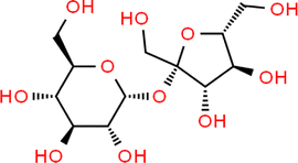
| Levoglucosan |
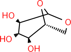
|
Wilhelmy plate | 25 | Aumann et al.17 | S = 0.5–1% | 72.36 |
| Pendant drop | — | Topping et al.44 | — | |||
| Wilhelmy plate | 20 | Tuckermann and Cammenga94 | — | |||
| Glutaric acid |
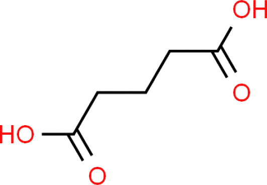
|
Pendant drop | — | Topping et al.44 | — | 72.36 |
| Wilhelmy plate | 20 | Lee and Hildemann95 | S < 0.3 mN m−1 | |||
| Pendant drop | 21 | Booth et al.45 | — | |||
| Wilhelmy plate | 25 | Aumann et al.17 | S = 0.5–1% | |||
| Wilhelmy plate | 24.85 | Boyer and Dutcher78 | S < 0.03 mN m−1 | |||
| Holographic optical tweezer | — | Boyer et al.53 | A = 1 mN m−1 | |||
| Holographic optical tweezer | — | Bzdek et al.96 | — | |||
| Wilhelmy plate | — | Bzdek et al.96 | — | |||
| Pendant drop | Ambient | Varga et al.97 | — | |||
| 1,2-ethanediol |

|
Bubble pressure tensiometer | 25 | Messow et al.98 | — | 71.97 |
| Methanol |

|
Nouy ring tensiometer | 25 | Basařova et al.99 | S < 0.2 mN m−1, A < 0.15 mN m−1 | 72.37 |
| Wilhelmy plate | 19.85 | Gliński et al.100 | ||||
| A = 0.4 mN m−1 | ||||||
| Drop volume tensiome | 25 | Maximino101 | S < 1% | |||
| Bubble pressure tensiometer | — | Semenov and Pokrovskaya102 | — | |||
| 1,6-hexanediol |

|
Capillary rise method | 25 | Romero et al.103 | S < 0.3 mN m−1 | 71.97 |
| Butyric acid |

|
Drop volume tensiometer | 25 | Granados et al.104 | S < 0.03 mN m−1 | 71.98 |
| Pendant drop | — | Suárez and Romero105 | S = 0.01 mN m−1 | |||
| Capillary rise method | 24.85 | Donaldson and Anderson106 | — | |||
| Nonanoic acid |
|
Nouy ring tensiometer | 21.85 | Lunkenheimer et al.107 | — | 72.46 |
| Bubble pressure tensiometer | — | Badban et al.108 | — | |||
| Triton X-100 |
|
Nouy ring tensiometer | 19.85 | Zdziennicka et al.109 | A = 0.3–0.7% | 72.76 |
| S < 0.2 mN m−1 | ||||||
3.3 Calculation of activity coefficients
For the calculation of activity coefficients the “Aerosol Inorganic–Organic Mixtures Functional groups Activity Coefficients” (AIOMFAC) model was used.110,111 This model combines the Pitzer model112 and the UNIFAC model83 and was designed with a focus on substances that are relevant in atmospheric science. It is available at http://www.aiomfac.caltech.edu/index.html.For organic solutions, using the AIOMFAC activity coefficients is equivalent to using UNIFAC. For alcohol groups, the new parametrization by Marcolli and Peter113 was used. For electrolytes (e.g. NaCl), AIOMFAC is based on the Pitzer model. The activity coefficients are ion specific and molality based with the 1-molal solution as the reference state. Hence, for the calculation of aNaCl, the mole fraction xNaCl was converted to molality and multiplied by the mean activity coefficient γNaCl = γNa+ = γCl−.110 The so-derived aNaCl is not bound to [0,1]. As a result, small modifications of the Li & Lu model and the Statistical model were necessary to fulfill the condition of σi = σ(xi = 1), while the Butler equation did not require any modifications (see Section 5 in ESI†). Due to the combination of the UNIFAC and the Pitzer model in AIOMFAC, the results in this study are valid, too, when activities are calculated with the UNIFAC model for organic solutes and the Pitzer model for inorganic solutes.
With AIOMFAC-based equilibrium calculations, liquid–liquid phase separation (LLPS) can also be predicted.114,115 For the solutions examined in this study, LLPS was predicted for strong surfactants, i.e. nonanoic acid and Triton X-100, for a certain concentration range. Substances with a strong amphiphilic structure are known to form structures of high surfactant content—known as micelles—above a certain concentration in the solution which is known as the critical micelle concentration (CMC). Since micelle formation can be regarded as a form of phase separation, we assumed that the onset of LLPS in AIOMFAC-based equilibrium calculations corresponds to the formation of micelles and thus LLPS was explicitly allowed when calculating the activity coefficients. Using activity coefficients of the phase separated system also led to much better fit performance than applying activities calculated for a one-phase system (i.e. suppressing LLPS). In the case of LLPS, it was assumed that the surfactant-rich phase determines the surface tension of the gas–liquid interface, based on its lower surface tension. As interfacial energies between the two liquid phases are of minor relevance in large droplets and bulk systems, they were neglected. Thus, the surface tension was calculated for the composition of the solute rich (outer) phase, which for nonanoic acid and Triton X-100 was the almost pure surfactant. The result of this approach is presented and discussed in Subsection 4.3.
4 Results and discussion
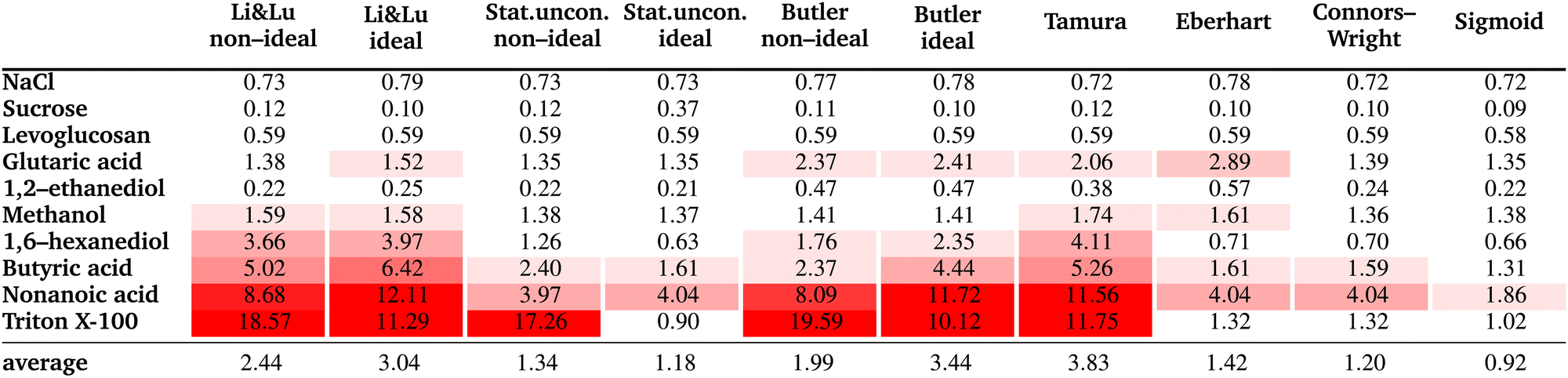
The resulting fit parameters for all substances and all models are shown in Table 3. In this table, for each fit the pure solute surface tension σi, which is determined either by fitting, taken from the literature, or set to the experimental value is also listed, since the other fit parameters are specific for this σi value. The corresponding RMSE values are summarized in Table 4. The results are presented and discussed by dividing the substances into the three groups: moderately surface active substances (1,2-ethanediol, methanol), substances with unknown σi (NaCl, levoglucosan, sucrose, glutaric acid) and intermediate to strong surface active substances (1,6-hexanediol, butyric acid, nonanoic acid, Triton X-100).| Li & Lunon-ideal | Li & Lu ideal | Stat. uncon. non-ideal | Stat. uncon. ideal | Butler non-ideal | Butler ideal | Tamura | Eberhart | Connors–Wright | Sigmoid | |||||
|---|---|---|---|---|---|---|---|---|---|---|---|---|---|---|
| Γ max (μmol m−2) | Γ max (μmol m−2) | r | K | r | K | A i (m2 mol−1) | A i (m2 mol−1) | q | S | a | b | p | d | |
| NaCl | −3.784 | −1.76 × 10⁷ | −0.013 | −0.084 | 9.25 × 10⁻⁵ | 0.983 | 6363 | 7024 | 3.50 | 0.848 | 0.934 | −0.031 | 1.08 | 1.16 |
| σ i (mN m−1) | 1821Fit | 156.4Fit | 97.42Fit | 4475Fit | 169.73Janz | 169.73Janz | 211.06Fit | 169.73Janz | 175.28Fit | 187.88Fit | ||||
| Sucrose | −0.588 | −2.357 | −28.25 | 0.99994 | −34.00 | 0.999999 | 63![[thin space (1/6-em)]](https://www.rsc.org/images/entities/char_2009.gif) 637 637 |
57027 |
6.24 | 6.613 | 0.993 | 0.0113 | 1.67 | 0.82 |
| σ i (mN m−1) | 85.45Fit | 87.54Fit | 99.54Fit | 98.48Fit | 81.80Fit | 82.90Fit | 80.08Fit | 83.58Fit | 121.13Fit | 105.25Fit | ||||
| Levoglucosan | 3.769 | 0.417 | 0.066 | −8.865 | 0.0973 | −58.90 | 306433 |
335696 |
4.34 | 60.13 | 0.983 | 1.0 | −2.03 | 1.84 |
| σ i (mN m−1) | 45.67Fit | 66.97Fit | 56.37Fit | 69.29Fit | 69.08Fit | 69.11Fit | 66.86Fit | 69.29Fit | 69.34Fit | 70.04Fit | ||||
| Glutaric | 2.304 | 1.602 | 6.707 | −1.256 | 9.567 | −1.750 | 217162 |
240178 |
3.94 | 73.02 | 0.991 | 0.377 | −1.57 | 0.67 |
| σ i (mN m−1) | 41.35Fit | 46.25Fit | 44.74Fit | 49.18Fit | 51.72Fit | 51.71Fit | 48.23Fit | 53.56Fit | 31.85Fit | 50.26Fit | ||||
| Ethanediol | 2.259 | 2.421 | 7.189 | −0.0436 | 6.034 | −0.245 | 44924 |
44624 |
1.96 | 6.894 | 0.907 | 0.747 | −0.51 | 0.66 |
| σ i = 47.00 mN m−1 | ||||||||||||||
| Methanol | 5.672 | 5.259 | 1.880 | −0.898 | 2.199 | −0.800 | 38529 |
38938 |
0.946 | 6.776 | 0.890 | 0.762 | −0.65 | 0.83 |
| σ i = 22.14 mN m−1 | ||||||||||||||
| Hexanediol | 1.257 | 0.800 | 0.00056 | −49.08 | 3.034 | −115.8 | 401369 |
525173 |
7.38 | 335.0 | 0.99698 | 1.0 | −2.53 | 0.94 |
| σ i = 42.60 mN m−1 | ||||||||||||||
| Butyric | 2.702 | 1.480 | 1.5 × 10⁻⁷ | −19.23 | 3.4 × 10⁻⁵ | −214.1 | 217095 |
332118 |
4.35 | 215.1 | 0.99528 | 1.0 | −2.30 | 1.21 |
| σ i = 26.51 mN m−1 | ||||||||||||||
| Nonanoic | 1.770 | 0.673 | 4.7 × 10⁻⁵ | −116.5 | 5.4 × 10⁻⁵ | −264239 |
512197 |
1139169 |
10.6 | 264242 |
0.999996 | 1.0 | −5.38 | 1.69 |
| σ i = 33.01 mN m−1 | ||||||||||||||
| TritonX100 | 0.874 | 0.4503 | 9.7 × 10⁻⁶ | −99.04 | 3.593 | −615468 |
2.7 × 10⁸ | 1968337 |
18.0 | 3153538 |
0.9999997 | 1.0 | −6.52 | 0.87 |
| σ i = 33.80 mN m−1 | ||||||||||||||
|
4.1 Moderately surface active substances
As pure liquids, 1,2-ethanediol and methanol both have a surface tension σi that is substantially lower than that of water. Consequently, in an aqueous solution with these compounds, the surface tension is lower than σw, but the deviation from a linear mixing rule is not very large. Thus, the preference of these substances to partition to the surface of the solution is only moderate. The continuously decreasing surface tension with increasing solute mole fraction of these moderately surface active substances is reproduced well by all models (see Fig. 3) resulting in low RMSE values (<2 mN m−1). The higher RMSE values for methanol than for 1,2-ethanediol are the result of the larger scatter of its experimental data. The ideal and non-ideal versions of the models using activity coefficients lead to very similar RMSE values, since 1,2-ethanediol and methanol mix almost ideally with water. This result suggests that the benefit of activity coefficients is not clear for these substances, and the additional effort of calculating them is not justified.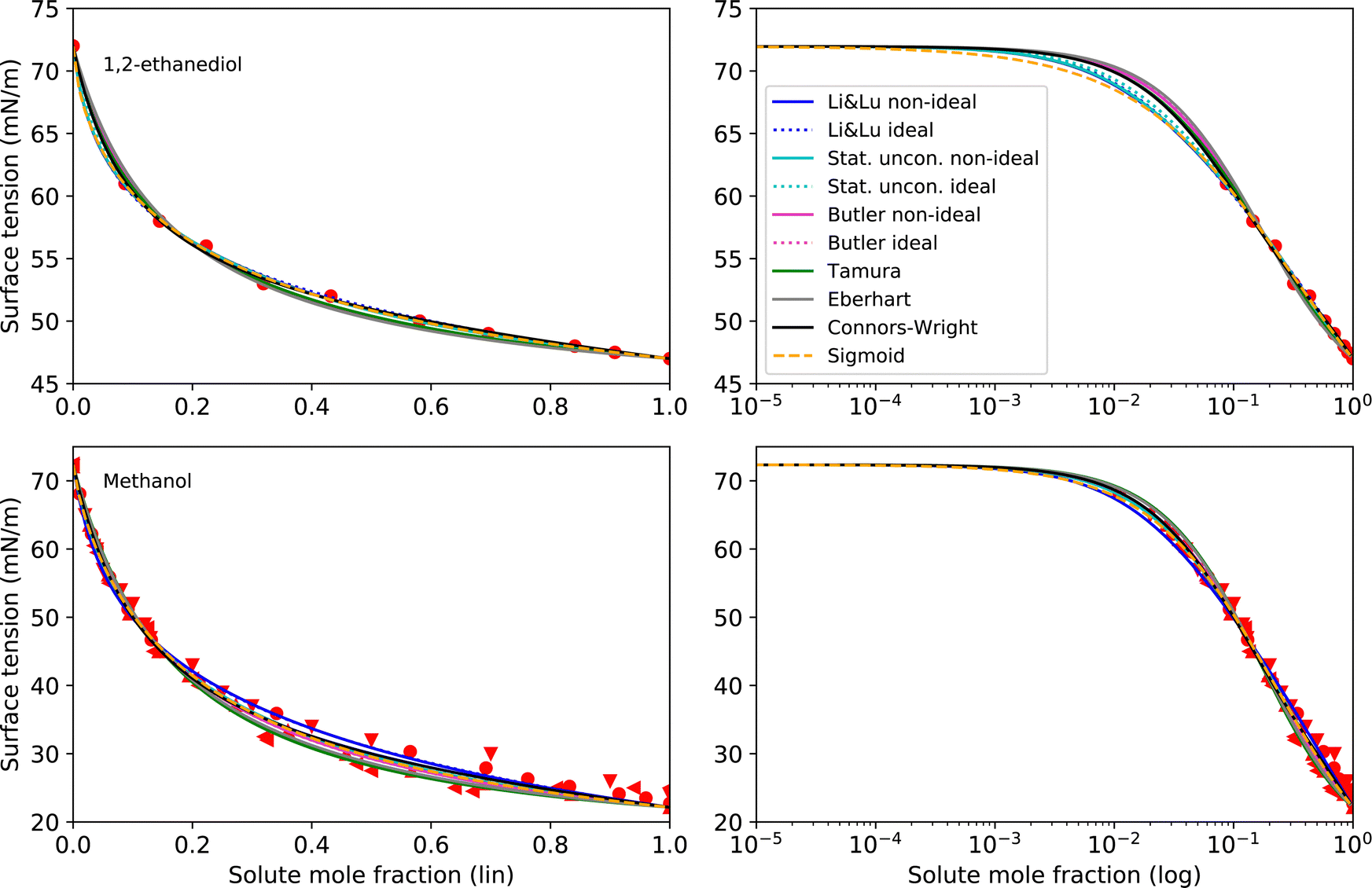 | ||
| Fig. 3 Surface tension fits (lines) and experimental data (red symbols) for 1,2-ethanediol and methanol on linear (left) and logarithmic scales (right). Different symbols of the experimental data refer to different sources (see Table 2 and Fig. S2 in ESI†). | ||
4.2 Substances with unknown σi
For NaCl, sucrose, levoglucosan, and glutaric acid, the surface tension of the pure liquid substance σi is not known, because these substances crystallize in the bulk at room temperature. Yet, the surface tension models we examine in this study are, directly or indirectly, a function of σi. While for bulk systems, the modelling can be restricted to concentrations below the solubility limit, for small droplets like aerosol particles, modelling beyond the solubility limit is required as these particles can strongly supersaturate. Smooth water uptake and loss of levitated levoglucosan particles during humidity cycles suggests that they do not crystallize at all and remain liquid at room temperature.117 Therefore, σi of levoglucosan should be considered a real quantity, but one that has not yet been measured. In contrast, glutaric acid and NaCl have been observed to eventually crystallize even in micrometer-sized droplets118,119 and sucrose transforms into a glass120 at high concentrations. For these three substances, σi can be considered a hypothetical quantity and thus, priority should be laid on accurately modelling the range of concentrations that can be realized. Moreover, in semi-empirical modelling, other fit parameters may compensate for differences in the choice of σi thereby allowing good fit performance independent of the exact choice of σi. Due to this dependence of the fit parameters on the choice of σi, especially in cases where σi is not well constrained, its value employed in the surface tension parameterization needs to be reported together with the other fit parameters to ensure reproducibility in modelling surface tensions by other groups. Note that Topping et al.44 found a high sensitivity in the choice of σi when they used predictive models, because in this case, the model has no fit parameters to ensure the reproduction of the data.The different options to obtain a value for σi include:
(i) Extrapolate from concentration-dependent measurements with a thermodynamic model (i.e. by fitting σi).
(ii) Resort to measurements of σi at a higher temperature where the substance is liquid and extrapolate to the desired temperature.
(iii) Use prediction tools like the Macleod–Sugden correlation or the corresponding states correlation (see Poling et al.59) based on physical properties like density, boiling point, and critical molar volume.
(iv) Use group contribution approaches and artificial neural network (ANN) models fed with experimental data from similar substances (derivation from other substances).
Making σi a fit parameter (option i) leads to the best RMSE values, due to having one additional adjustable parameter. Therefore, here we present surface tension fits with all tested models and for all tested substances, that use σi as a fit parameter with two exceptions: For the Eberhart model and the Butler equation, fitting NaCl with unknown σi was unsuccessful due to numerical issues (too many free parameters). In this case, σi was taken from an extrapolation of the temperature function by Janz116 (option ii), which is based on molten salt measurements. Extrapolation of this function gives a value of σNaCl = 169.73 mN m−1 at T = 25 °C, which is frequently used for surface tension parameterizations of NaCl solutions.18,26,73,121,122 The results following this approach for NaCl, sucrose, levoglucosan and glutaric acid are shown in Fig. 4 and the corresponding parameters in Table 3.
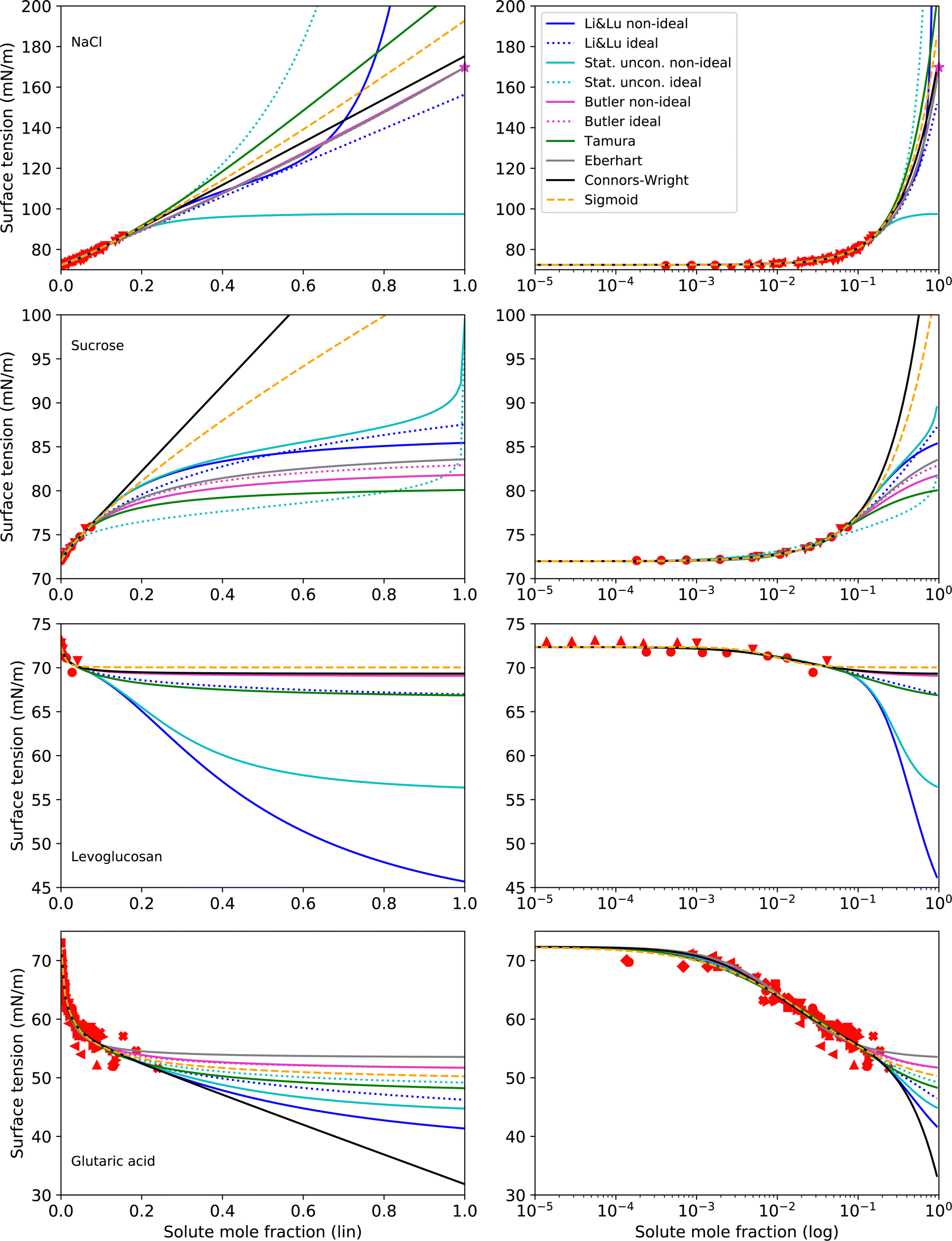 | ||
| Fig. 4 Surface tension fits (lines) and experimental data (red symbols) for substances with unknown σi on linear (left) and logarithmic (right) x-axis scales. All models use σi as a fit parameter except for NaCl, where the Eberhart model and the Butler equation use σi = 169.73 mN m−1 (purple star), as suggested by a temperature extrapolation from molten salt measurements.116 No values for σi of sucrose could be found in the literature. For levoglucosan, a prediction with the Macleod–Sugden correlation and Yens–Wood densities suggests a value of σi = 22.71 mN m−1.44 Values for σi of glutaric acid reported in the literature include 43.22 mN m−1 (NIST, temperature extrapolation),123 38.88 mN m−1 (Macleod–Sugden and Yens–Wood) and 56.1 mN m−1 (ACDlabs Chemsketch 5.0).44 Different symbols of the experimental data refer to different sources (see Table 2 and Fig. S2 in ESI†). Note that for NaCl and glutaric acid, the curve fits of the non-ideal and ideal versions of the Butler equation completely overlay. For levoglucosan, the curve fits of the models Stat. uncon. ideal, Butler ideal, Eberhart and Connors–Wright completely overlay. | ||
As can be seen from Fig. 4, fitting σi with the various models results in a large range of σi values. Therefore, when the surface tension of solutions in the supersaturated concentration range is of interest, a better constraint of σi is desireable. For NaCl, an alternative to fitting σi is given by temperature extrapolation following Janz,116 as mentioned above.
For sucrose and levoglucosan, no data is available for an extrapolation from higher temperature (ii), and sucrose even decomposes before melting. Prediction tools (iii) also fail because physical properties like boiling point and critical molar volume data cannot be determined. In this case, only group contribution approaches or ANN models can be used (iv), either to predict the lacking quantities for option (iii) or to directly predict σi. However, no model to directly predict σi was available in the literature for sugars and polyols, evidencing a lack of research in this field. For levoglucosan, a value of σlevoglucosan = 22.71 mN m−1 calculated with Macleod–Sugden's method and Yens–Wood densities could be found,44 which seems too low in comparison with molecules of similar structures like sugars.
For glutaric acid, several predictions of its pure liquid surface tension σglutaric can be found in the literature. Mulero et al.123 carefully screened surface tension data of pure organic acids and suggest functions for the temperature dependence for the NIST REFPROP program.124 The data thereby is mostly based on predictions with the Macleod–Sugden method (iii) at higher temperature, where the acids are liquid. An extrapolation to room temperature (ii) results in σglutaric = 43.22 mN m−1 at T = 25 °C. Using the Macleod–Sugden method combined with the predictive Yens–Wood method for the calculation of subcooled liquid densities, Topping et al.44 reported a value of σglutaric = 38.88 mN m−1 at T = 25 °C. The same authors report a value of σglutaric = 56.1 mN m−1 predicted by ACDlabs Chemsketch 5.0. This spread highlights the uncertainties related to σi for organic acids and the need for further research.
Since for sucrose, levoglucosan and glutaric acid, no good prediction of σi could be obtained by options (ii) to (iv), the question arises if option (i) can be used to estimate σi. The large spread in fitted σi values in Fig. 4 suggests that some models are less physically constrained and simply follow the trend of the data, while others seem to be more robust and less prone to predict unphysical σi values. Using the data from methanol and butyric acid, we tested the capability of the models to extrapolate to high concentrations by fitting the models to only a part of the experimental data (Section 6 in the ESI†). Comparing the thereby predicted σi with the actual σi of these two substances showed that the Butler equation seems to be a model that is relatively robust in extrapolating the surface tension even from very limited experimental data. However, the Butler equation seems to be strongly dependent on the activity coefficient model that is being used and only precise substance-specific activity coefficients would allow to actually examine the predictive capabilities of the Butler equation. From the extrapolation test and the fits for sucrose and levoglucosan in Fig. 4, it can also be seen that if the data are limited to too narrow of a concentration range, the uncertainty in the predicted σi values becomes very large for all models. A solution to this problem could be to take measurements of the surface tension at a higher temperature or to change to a solvent that allows for a higher solubility such that experimental data over a wider concentration range can be obtained, and thus providing a better prediction of σi. From the current study, we cannot yet recommend a final methodology to obtain precise surface tension fits for the supersaturated concentration range of crystallizing substances, but we suggest to test the aforementioned approaches in future studies.
4.3 Intermediate to strong surfactants
The surface tension curves for aqueous solutions of 1,6-hexanediol, butyric acid, nonanoic acid and Triton X-100 are characterized by a strong decrease in surface tension in a narrow, low concentration range and a plateauing of the surface tension at higher concentrations, as is characteristic for substances with strong surface partitioning. The concentration at which the surface tension curves change from a negative slope to a plateau at low surface tension marks the concentration at which the surface is fully covered with solute molecules and where for strongly amphiphilic molecules the formation of micelles in the bulk starts (CMC). While for 1,6-hexanediol and butyric acid, the CMC lies at xCMC ≈ 10−2 to 10−1, for nonanoic acid and Triton X-100 it is at a substantially lower concentration (xCMC ≈ 1 × 10⁻⁵), which is why we categorize the former as “intermediate surfactants” and the latter as “strong surfactants”.As can be seen in Fig. 5, the Li & Lu models, the Butler equation (ideal) and the Tamura model were not able to reproduce the steep surface tension decrease at low concentration for intermediate and even less so for strong surfactants. In contrast, with the Stat. uncon. ideal, Eberhart, Connors–Wright and Sigmoid models, the shape of the experimental data could be reproduced closely for both the intermediate and strong surfactants.
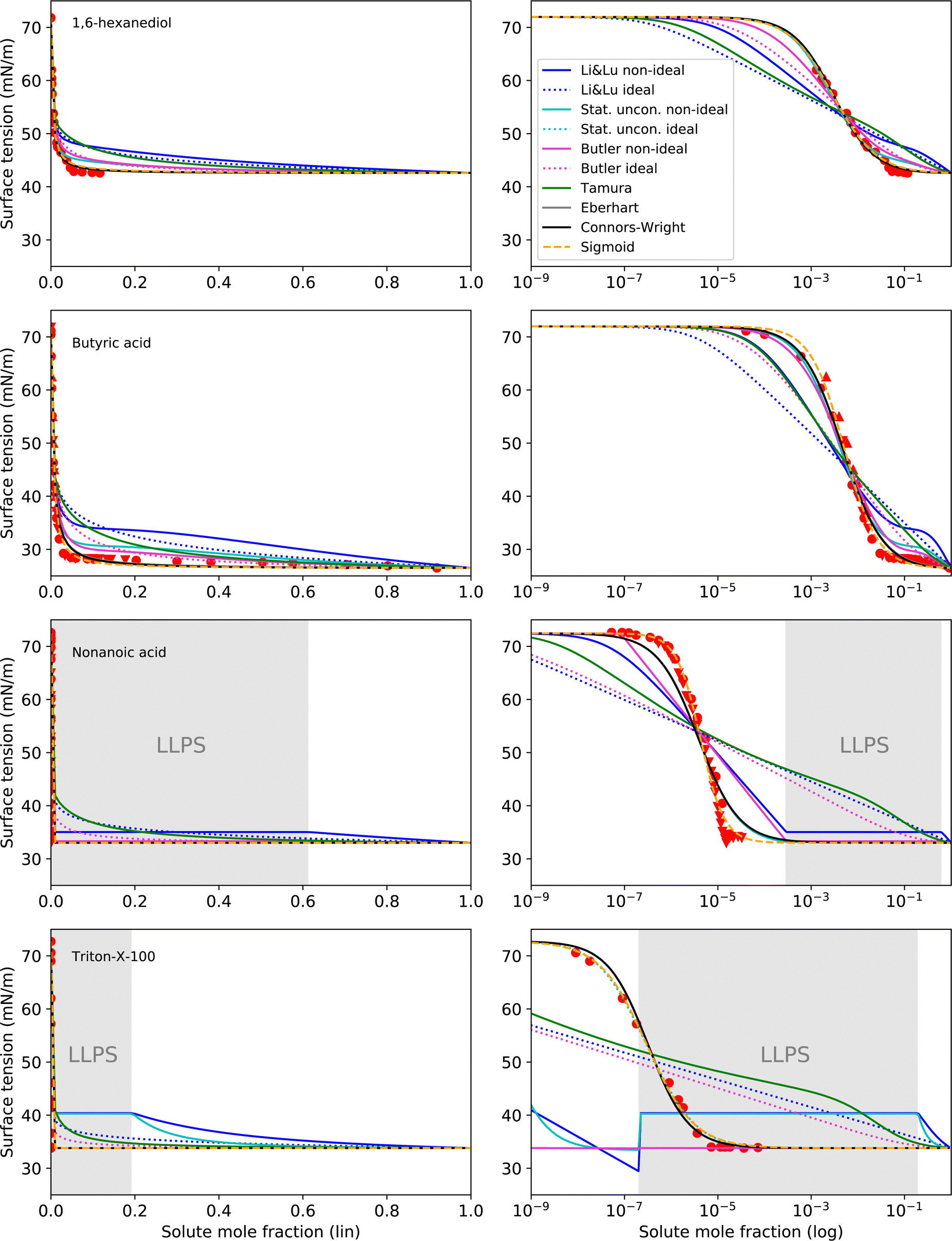 | ||
| Fig. 5 Surface tension fits (lines) and experimental data (red symbols) for intermediate to strong surface active substances on linear (left) and logarithmic (right) x-axis scale. Liquid–liquid phase separation (LLPS) was predicted by AIOMFAC for nonanoic acid and Triton X-100 in the grey shaded concentration range. Different symbols of the experimental data refer to different sources (see Table 2 and Fig. S2 in ESI†). Note that the curve fits of the models Stat. uncon. ideal, Eberhart and Connors–Wright partly or completely overlay. | ||
The performance of the models using activity coefficients (Butler, Stat. uncon., Li & Lu, all non-ideal) was found to be highly dependent on the activity coefficients and LLPS prediction by AIOMFAC. As can be seen in the fits for nonanoic acid in Fig. 5, the LLPS from xi = 2.8 × 10⁻⁴ to xi = 0.613 (grey-shaded area) is responsible for the abrupt changes in σ at the left and right end of the LLPS region and the plateau in between for these models. The Butler equation (non-ideal) has an additional kink at xi ≈ 10−7. To understand this distinctive curve shape, the reader is reminded that in the Butler theory, the liquid phase is divided into a bulk phase and a surface phase. At the kink at xi ≈ 10−7, the composition of the surface phase xsurfi, which is restricted—same as the bulk phase—to compositions that do not phase separate, changes abruptly from surfactant-poor (xsurfi = 2.8 × 10⁻⁴) to surfactant-rich (xsurfi = 0.613). In the subsequent decrease in σ, the surface phase further enriches in solute, until, at xi = 0.613, the bulk eventually phase separates. At this point, the surfactant-rich (bulk) phase determines the surface tension. The resulting step-like surface tension fit of the non-ideal Butler equation nicely reproduces the steep σ decrease and the abrupt plateauing of the nonanoic acid data, but only a close agreement of the actual CMC and the predicted LLPS onset would ensure a good fit. In the case of nonanoic acid, the xi of LLPS onset predicted by AIOMFAC is slightly too high. Since AIOMFAC is a group contribution model, the activity and LLPS predictions for a single substance cannot be expected to match the data exactly.
While for nonanoic acid, AIOMFAC predicts the LLPS onset at a higher mole fraction than the actual CMC, for Triton X-100, the opposite is the case. For Triton X-100, AIOMFAC predicts LLPS from xi = 2 × 10⁻⁷ to xi = 0.192, while the CMC is found at xCMC ≈ 10−5. As a result, no proper fits could be made with the models using non-ideality. A solution to this problem could be to introduce an additional fit parameter that serves to correct the AIOMFAC activity coefficients for the substance of concern in order to match the onset of LLPS with the CMC.
While non-ideal and ideal model versions achieved similar RMSE values for 1,2-ethanediol and methanol, the non-ideal versions of the Li & Lu model and the Butler equation indeed improved the fit performance for intermediate and strong surfactants, since for these substances non-ideality is much more pronounced. This is not the case for the Statistical unconstrained model, probably due to the loss of its physical basis, since we used the parameters in an unphysical way (i.e. allowing K to be negative). The reader is reminded that a physically correct application of the Statistical model for surface active substances leads to the same results as the Li & Lu model.
4.4 Strengths and weaknesses of the models
Finally, we discuss the strengths and weaknesses of the models with regard to programming and computational effort, meaning and precision of fit parameters, predictive capabilities, application to multi-component solutions, extrapolation, and derivation of the surface composition.All models tested in this paper are mathematically rather simple equations and thus not very computationally expensive and numerically very stable. The time to write the code for fitting the models and to debug it was mostly short and the resulting code not very long. The Butler equation is the only model that raised some numerical difficulties and took a considerable amount of time to be coded, debugged and executed for the fitting to experimental data. The reasons are that (i) a system of equations needs to be solved instead of an analytical expression, (ii) the calculation of activity coefficients is required, and (iii) activity values too close to zero must be detected by the code with an appropriate threshold to avoid errors from the logarithmic function trying to solve for zero.
The Eberhart, Connors–Wright, Stat. uncon. ideal and Sigmoid models all fit the surface tension data of all studied substances accurately. The versatility of these models ensures that a single framework of fit parameters can be chosen to report the effect of different solutes on surface tension. All solutes can then be compared quantitatively to each other within that framework to lend insight into, for example, which are more surface active. To facilitate a comparison, the fit parameters should be easy to interpret and convenient to report. The fit parameters of the Eberhart and Connors–Wright models require mathematical manipulation to describe their influence on the shape of the surface tension curve (e.g., Fig. 1). Additionally, strong surfactants like Triton-X-100 bring these models to the limit of their fitting capacity as manifested by the many significant digits that must be reported for the fit parameters to describe the data accurately (e.g. for the Connors–Wright model, a = 0.9999997). Alternatively, the Sigmoid model has tangible fit parameters (the concentration at the inflection point and the CMC), and only a few significant digits are required to ensure high precision. Combined with its high accuracy, the Sigmoid model is easily interpretable and convenient, making it an elegant tool for the numerical reporting and comparison of solutes surface activeness.
Compared to the Szyszkowski–Langmuir equation, which is often used in atmospheric sciences, the Sigmoid model provides a smooth curve over the whole concentration range, while the Szyszkowski–Langmuir equation needs to be combined with a constant value at concentrations above the CMC, which can be challenging for numerical solvers.
The Sigmoid model, being a purely empirical model, requires experimental data, i.e. it has no predictive capabilities at the current state of development. Possible relationships between molecular properties and the fit parameters have yet to be researched. Such relationships have been found for the Statistical model for alcohols, polyols and electrolytes. Similarly, the Tamura model suggests predictive model parameters for certain solute groups. Only the Butler equation provides a fully predictive surface tension model through thermodynamic derivation that is valid for all types of solutes. However, it requires activity coefficients and molar surface areas of all substances in the mixture. Due to the difficulties in obtaining precise values for these, the predictive capabilities of the Butler equation are often unsatisfactory, and a measurement of the surface tension is a more reliable option compared to a prediction based on molecular properties.
The ability of the models to extrapolate to concentrations without experimental data was discussed in Section 4.2 and a preliminary extrapolation test suggests that the Butler equation is the most robust model to extrapolate (ESI† Section 6), possibly due to a strong thermodynamic background. Yet, more research is required to reach a more definitive conclusion.
For processes like heterogeneous surface reactions or bulk depletion in tiny droplets, the surface composition xsurfi corresponding to a certain bulk composition is required additionally to surface tension. In the Butler equation, asurfi is a direct model output and allows to back-calculate xsurfi. The Statistical model allows a derivation of xsurfi as a function of ai and the fit parameters based on eqn (8) in Wexler and Dutcher.50 Also for the Li & Lu model, a derivation of the number of moles in the surface and the bulk has been suggested.46 The Eberhart and the Connors–Wright models assume that a simple linear mixing rule
| σ = σixsurfi + σwxsurfw | (28) |
 | (29) |
 | (30) |
 | (31) |
5. Summary and conclusions
In this study, we reviewed empirical, semi-empirical and thermodynamic surface tension models for aqueous solutions. Furthermore, we derived a new empirical model that is based on the logistic function (Sigmoid model). We compared the ability of six frequently-used models as well as the proposed Sigmoid model to fit experimental surface tension data of binary aqueous mixtures. Our study revealed the following findings:• The Sigmoid model was found to have the best overall fit performance of all models, with an average RMSE of 0.92 mN m−1 and individual RMSE values <2 mN m−1. For all tested substances, the experimental data could be excellently reproduced (see Fig. 6). We therefore recommend this model to describe experimental surface tension data with an analytical equation.
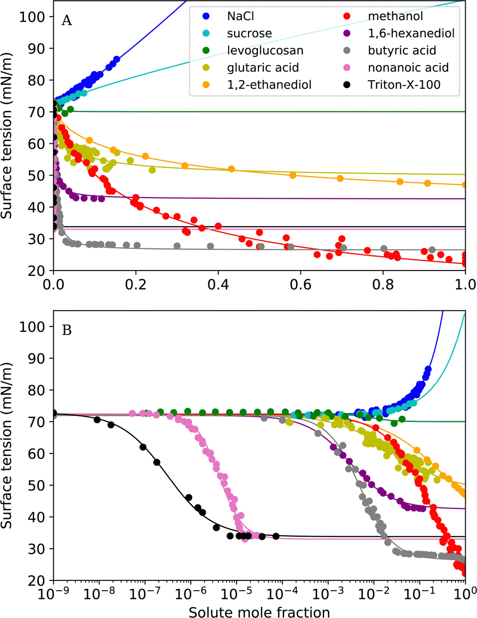 | ||
| Fig. 6 Surface tension fits with the Sigmoid model for all tested substances (A) on a linear x-axis scale (B) on a logarithmic x-axis scale. | ||
• From the models proposed in the literature, the Connors–Wright model was found to be the most versatile in fitting different curve shapes. In contrast to the empirical Sigmoid model, it has a simple thermodynamic basis and a formulation for multi-component solutions. Its capability to predict the surface tension of multi-component solutions for a wide variety of compounds, however, remains to be tested.
• For weakly surface active substances like 1,2-ethanediol or methanol, all seven models achieved good results with RMSE values <2 mN m−1. The Li & Lu model, the Tamura model and the Butler equation (ideal) were found not to be able to fit the surface tension of surfactants. The Statistical model is equivalent to the Li & Lu model for intermediate and strong surfactants when restricting the fit parameters to values within the physically meaningful limits. An unphysical usage of the model by allowing negative values for K leads to a model with good fit performance, especially when assuming ideality (“Stat. uncon. ideal”) although lacking a thermodynamic basis.
• For substances that are solid at room temperature, the pure liquid surface tension σi is unknown. We discussed various options to estimate its value, including to make σi a fit parameter, which means estimating its value from an extrapolation of the experimental data using one of the tested surface tension models. Depending on the model, the values obtained for σi by such extrapolation are more or less subject to physical constraints. According to our analysis, the Butler equation seems to be a robust model for extrapolating to unknown concentrations as long as accurate, substance-specific activity coefficients can be provided. Overall, more research about the various methods of obtaining σi is clearly needed, especially for sugars.
• AIOMFAC has proven a useful tool to calculate activity coefficients for a broad range of substances including organic and inorganic substances. For strong surfactants, AIOMFAC predicts a liquid–liquid phase separation into one surfactant-rich and a water-rich phase within a wide concentration range which can be interpreted as the formation of micelles. This prediction of micelle formation (in the form of a liquid–liquid phase separation) is crucial for surface tension fits for strong surfactants but it is not very accurate in AIOMFAC, since AIOMFAC is a group contribution method. A solution to this problem could be a tuning of the activity coefficients to the specific substance. This could be the subject of future work.
To conclude, the Sigmoid model was found to excellently reproduce the surface tension of binary aqueous solutions over the whole concentration range and for a broad range of solutes. This allows modelling the surface tension of aqueous solutions in a universal and simple way, which can be helpful in many fields. Further research should be directed to extending the Sigmoid model to capture multi-component solutions and to obtaining better estimates of the pure liquid surface tension σi of crystallizing substances.
Data availability statement
Data for this paper, including the experimental surface tension data, activity coefficients calculated with AIOMFAC, fitted curves, and fit parameters are available at https://doi.org/10.5281/zenodo.7548346.Author contributions
J. K. reviewed the literature, analyzed the models, visualized the results and wrote the original draft. N. S. and C. M. directly supervised this work and contributed to the methodology and validation and C. M. acquired the funding. M. H., C. F. and B. N. provided the surface tension data. T. P. contributed with resources and supervising. All authors contributed to conceptualization and writing (review & editing), and all authors have approved the final version of the paper.Conflicts of interest
There are no conflicts to declare.Acknowledgements
We thank Andreas Zuend for providing the AIOMFAC code and initial support for using it. We furthermore acknowledge programming support from Sylvaine Ferrachat as well as helpful discussions with Cari Dutcher, Shihao Liu, Hallie Chelmo and Ryan Schmedding. This research has been funded by the Swiss National Science Foundation (SNF; grant no. 200021L_197149) and the French National Research Agency (ANR-20-CE93-0008) as part of the binational ORACLE project. N. S. was supported by an ETH Postdoctoral Fellowship (20-1 FEL-46) and a Natural Sciences and Engineering Research Council of Canada (NSERC) Postdoctoral Fellowship.References
- S. Syeda, A. Afacan and K. Chuang, Chem. Eng. Res. Des., 2004, 82, 762–769 CrossRef CAS
.
- J. Pérez-Gil, Biochim. Biophys. Acta, Biomembr., 2008, 1778, 1676–1695 CrossRef PubMed
- O. Mc Callion, K. Taylor, M. Thomas and A. Taylor, Int. J. Pharm., 1996, 129, 123–136 CrossRef
- K. A. Wokosin, E. L. Schell and J. A. Faust, Environ. Sci.: Atmos., 2022, 2, 775–828 Search PubMed
- R. C. Tolman, J. Chem. Phys., 1949, 17, 333–337 CrossRef CAS
- H. D. Lee and A. V. Tivanski, Annu. Rev. Phys. Chem., 2021, 72, 235–252 CrossRef CAS PubMed
- R. Power and J. Reid, Rep. Prog. Phys., 2014, 77, 074601 CrossRef PubMed
- B. Minofar, P. Jungwirth, M. R. Das, W. Kunz and S. Mahiuddin, J. Phys. Chem. C, 2007, 111, 8242–8247 CrossRef CAS
- S. Mahiuddin, B. Minofar, J. M. Borah, M. R. Das and P. Jungwirth, Chem. Phys. Lett., 2008, 462, 217–221 CrossRef CAS
- J. C. Neyt, A. Wender, V. Lachet, A. Ghoufi and P. Malfreyt, J. Chem. Phys., 2013, 139, 024701 CrossRef CAS PubMed
- N. S. Mousavi, B. Vaferi and A. Romero-Martínez, Ind. Eng. Chem. Res., 2021, 60, 10354–10364 CrossRef CAS
- Z. Nieto, V. M. K. Kotteda, A. Rodriguez, S. S. Kumar, V. Kumar and A. Bronson, Proceedings of the 5th Joint US-European Fluids Engineering Division Summer Meeting, ASME, 2018, vol. 3, p. V003T21A003.
- M. Pierantozzi, A. Mulero and I. Cachadiña, Molecules, 2021, 26, 1636 CrossRef CAS PubMed
- T. Soori, S. M. Rassoulinejad-Mousavi, L. Zhang, A. Rokoni and Y. Sun, Fluid Phase Equilib., 2021, 538, 113012 CrossRef CAS
- I. Egry, E. Ricci, R. Novakovic and S. Ozawa, Adv. Colloid Interface Sci., 2010, 159, 198–212 CrossRef CAS PubMed
- A. Asa-Awuku, A. P. Sullivan, C. J. Hennigan, R. J. Weber and A. Nenes, Atmos. Chem. Phys., 2008, 8, 799–812 CrossRef CAS
- E. Aumann, L. Hildemann and A. Tabazadeh, Atmos. Environ., 2010, 44, 329–337 CrossRef CAS
- B. R. Bzdek, J. P. Reid, J. Malila and N. L. Prisle, Proc. Natl. Acad. Sci., 2020, 117, 8335–8343 CrossRef CAS PubMed
- M. Facchini, M. Mircea, F. Sandro and R. Charlson, Nature, 1999, 401, 257–259 CrossRef CAS
- M. R. Giordano, D. Z. Short, S. Hosseini, W. Lichtenberg and A. A. Asa-Awuku, Environ. Sci. Technol., 2013, 47, 10980–10986 CrossRef CAS PubMed
- S. Henning, T. Rosenørn, B. D'Anna, A. A. Gola, B. Svenningsson and M. Bilde, Atmos. Chem. Phys., 2005, 5, 575–582 CrossRef CAS
- H. Kokkola, R. Sorjamaa, A. Peräniemi, T. Raatikainen and A. Laaksonen, Geophys. Res. Lett., 2006, 33, L10816 CrossRef
- T. B. Kristensen, N. L. Prisle and M. Bilde, Atmos. Res., 2014, 137, 167–175 CrossRef CAS
- Z. Li, A. L. Williams and M. Rood, J. Atmos. Sci., 1998, 55, 1859–1866 CrossRef
- J. J. Lin, J. Malila and N. L. Prisle, Environ. Sci.: Processes Impacts, 2018, 20, 1611–1629 RSC
- J. J. Lin, T. B. Kristensen, S. M. Calderón, J. Malila and N. L. Prisle, Environ. Sci.: Processes Impacts, 2020, 22, 271–284 RSC
- A. Z. Mazurek, S. J. Pogorzelski and A. D. Kogut, Atmos. Environ., 2006, 40, 4076–4087 CrossRef CAS
- R. McGraw and J. Wang, J. Chem. Phys., 2021, 154, 024707 CrossRef CAS PubMed
- H. S. Morris, V. H. Grassian and A. V. Tivanski, Chem. Sci., 2015, 6, 3242–3247 RSC
- B. Noziere, C. Baduel and J.-L. Jaffrezo, Nat. Commun., 2014, 5, 3335 CrossRef PubMed
- S. S. Petters and M. D. Petters, J. Geophys. Res.: Atmos., 2016, 121, 1878–1895 CrossRef CAS
- N. Prisle, T. Raatikainen, R. Sorjamaa, B. Svenningsson, A. Laaksonen and M. Bilde, Tellus B, 2008, 60, 416–431 CrossRef
- N. L. Prisle, T. Raatikainen, A. Laaksonen and M. Bilde, Atmos. Chem. Phys., 2010, 10, 5663–5683 CrossRef CAS
- N. L. Prisle, M. Dal Maso and H. Kokkola, Atmos. Chem. Phys., 2011, 11, 4073–4083 CrossRef CAS
- N. L. Prisle, A. Asmi, D. Topping, A.-I. Partanen, S. Romakkaniemi, M. Dal Maso, M. Kulmala, A. Laaksonen, K. E. J. Lehtinen, G. McFiggans and H. Kokkola, Geophys. Res. Lett., 2012, 39, L05802 CrossRef
- N. L. Prisle and B. Molgaard, Atmospheric Chemistry and Physics Discussions, 2018, 2018, 1–23 Search PubMed
- N. L. Prisle, Atmos. Chem. Phys., 2021, 21, 16387–16411 CrossRef CAS
- T. Raatikainen and A. Laaksonen, Geosci. Model Dev., 2011, 4, 107–116 CrossRef
- S. Romakkaniemi, H. Kokkola, J. N. Smith, N. L. Prisle, A. N. Schwier, V. F. McNeill and A. Laaksonen, Geophys. Res. Lett., 2011, 38, L03807 CrossRef
- A. Schwier, D. Mitroo and V. F. McNeill, Atmos. Environ., 2012, 54, 490–495 CrossRef CAS
- R. Sorjamaa and A. Laaksonen, J. Aerosol Sci., 2006, 37, 1730–1736 CrossRef CAS
- R. Tuckermann, Atmos. Environ., 2007, 41, 6265–6275 CrossRef CAS
- Z. Li and B. C.-Y. Lu, Chem. Eng. Sci., 2001, 56, 2879–2888 CrossRef CAS
- D. O. Topping, G. B. McFiggans, G. Kiss, Z. Varga, M. C. Facchini, S. Decesari and M. Mircea, Atmos. Chem. Phys., 2007, 7, 2371–2398 CrossRef CAS
- A. M. Booth, D. O. Topping, G. McFiggans and C. J. Percival, Phys. Chem. Chem. Phys., 2009, 11, 8021–8028 RSC
- D. Topping, Geosci. Model Dev., 2010, 3, 635–642 CrossRef
- B. von Szyszkowski, Z. Phys. Chem., 1908, 64U, 385–414 CrossRef
- I. Langmuir, J. Am. Chem. Soc., 1917, 39, 1848–1906 CrossRef CAS
- A. N. Schwier, G. A. Viglione, Z. Li and V. Faye McNeill, Atmos. Chem. Phys., 2013, 13, 10721–10732 CrossRef
- A. S. Wexler and C. S. Dutcher, J. Phys. Chem. Lett., 2013, 4, 1723–1726 CrossRef CAS PubMed
- H. Boyer, A. Wexler and C. Dutcher, J. Phys. Chem. Lett., 2015, 6, 3384–3389 CrossRef CAS PubMed
- H. C. Boyer and C. S. Dutcher, J. Phys. Chem. A, 2017, 121, 4733–4742 CrossRef CAS PubMed
- H. C. Boyer, B. R. Bzdek, J. P. Reid and C. S. Dutcher, J. Phys. Chem. A, 2017, 121, 198–205 CrossRef CAS PubMed
- R. Miles, M. Glerum, H. Boyer, J. Walker, C. Dutcher and B. Bzdek, J. Phys. Chem. A, 2019, 123, 3021–3029 CrossRef CAS PubMed
- J. A. V. Butler, Proc. R. Soc. London, Ser. A, 1932, 135, 348–375 CAS
- F. B. Sprow and J. M. Prausnitz, Trans. Faraday Soc., 1966, 62, 1105–1111 RSC
- J. T. Suarez, C. Torres-Marchal and P. Rasmussen, Chem. Eng. Sci., 1989, 44, 782–785 CrossRef CAS
- M. S. C. S. Santos and J. C. R. Reis, ACS Omega, 2021, 6, 21571–21578 CrossRef CAS PubMed
-
B. E. Poling, J. M. Prausnitz and J. P. OConnell, Properties of Gases and Liquids, McGraw-Hill Education, New York, 5th edn, 2001, ch. 12 Search PubMed
- Z.-B. Li, Y.-G. Li and J.-F. Lu, Ind. Eng. Chem. Res., 1999, 38, 1133–1139 CrossRef CAS
- Y.-F. Hu and H. Lee, J. Colloid Interface Sci., 2004, 269, 442–448 CrossRef CAS PubMed
- X. Cai and R. J. Griffin, J. Atmos. Chem., 2005, 50, 139–158 CrossRef CAS
- J. Werner, J. Julin, M. Dalirian, N. L. Prisle, G. Öhrwall, I. Persson, O. Björneholm and I. Riipinen, Phys. Chem. Chem. Phys., 2014, 16, 21486–21495 RSC
- J. Werner, M. Dalirian, M.-M. Walz, V. Ekholm, U. Wideqvist, S. Lowe, G. Ohrwall, I. Persson, I. Riipinen and O. Björneholm, Environ. Sci. Technol., 2016, 50, 7434–7442 CrossRef CAS PubMed
- M. Tamura, M. Kurata and H. Odani, Bull. Chem. Soc. Jpn., 1955, 28, 83–88 CrossRef CAS
- J. G. Eberhart, J. Phys. Chem., 1966, 70, 1183–1186 CrossRef CAS
- J. Shereshefsky, J. Colloid Interface Sci., 1967, 24, 317–322 CrossRef CAS
- N. Shardt and J. A. W. Elliott, Langmuir, 2017, 33, 11077–11085 CrossRef CAS PubMed
- K. A. Connors and J. L. Wright, Anal. Chem., 1989, 61, 194–198 CrossRef CAS
- N. Shardt, Y. Wang, Z. Jin and J. A. Elliott, Chem. Eng. Sci., 2021, 230, 116095 CrossRef CAS
- L. Chunxi, W. Wenchuan and W. Zihao, Fluid Phase Equilib., 2000, 175, 185–196 CrossRef CAS
- A.-P. Hyvärinen, H. Lihavainen, A. Gaman, L. Vairila, H. Ojala, M. Kulmala and Y. Viisanen, J. Chem. Eng. Data, 2006, 51, 255–260 CrossRef
- J. Vanhanen, A.-P. Hyvärinen, T. Anttila, T. Raatikainen, Y. Viisanen and H. Lihavainen, Atmos. Chem. Phys., 2008, 8, 4595–4604 CrossRef CAS
-
R. Defay, I. Prigogine, A. Bellemans and D. Everett, Surface Tension and Adsorption, Wiley, 1966 Search PubMed
- R. Sorjamaa, B. Svenningsson, T. Raatikainen, S. Henning, M. Bilde and A. Laaksonen, Atmos. Chem. Phys., 2004, 4, 2107–2117 CrossRef CAS
- J. A. W. Elliott, J. Phys. Chem. B, 2020, 124, 10859–10878 CrossRef CAS PubMed
- I. Langmuir, J. Am. Chem. Soc., 1918, 40, 1361–1403 CrossRef CAS
- H. C. Boyer and C. S. Dutcher, J. Phys. Chem. A, 2016, 120, 4368–4375 CrossRef CAS PubMed
- S. Liu and C. S. Dutcher, J. Phys. Chem. A, 2021, 125, 1577–1588 CrossRef CAS PubMed
- C. S. Dutcher, X. Ge, A. S. Wexler and S. L. Clegg, J. Phys. Chem. C, 2011, 115, 16474–16487 CrossRef CAS
- C. S. Dutcher, X. Ge, A. S. Wexler and S. L. Clegg, J. Phys. Chem. C, 2012, 116, 1850–1864 CrossRef CAS
- C. S. Dutcher, X. Ge, A. S. Wexler and S. L. Clegg, J. Phys. Chem. A, 2013, 117, 3198–3213 CrossRef CAS PubMed
- A. Fredenslund, R. L. Jones and J. M. Prausnitz, AIChE J., 1975, 21, 1086–1099 CrossRef CAS
- D. E. Goldsack and B. R. White, Can. J. Chem., 1983, 61, 1725–1729 CrossRef CAS
- M. Vermot des Roches, A. E. Gheribi and P. Chartrand, Calphad, 2019, 65, 326–339 CrossRef CAS
- A. Dobosz, R. Novakovic and T. Gancarz, J. Mol. Liq., 2021, 343, 117646 CrossRef CAS
- G. M. Wilson, J. Am. Chem. Soc., 1964, 86, 127–130 CrossRef CAS
- P. Virtanen, R. Gommers, T. E. Oliphant, M. Haberland, T. Reddy, D. Cournapeau, E. Burovski, P. Peterson, W. Weckesser, J. Bright, S. J. van der Walt, M. Brett, J. Wilson, K. J. Millman, N. Mayorov, A. R. J. Nelson, E. Jones, R. Kern, E. Larson, C. J. Carey, İ. Polat, Y. Feng, E. W. Moore, J. VanderPlas, D. Laxalde, J. Perktold, R. Cimrman, I. Henriksen, E. A. Quintero, C. R. Harris, A. M. Archibald, A. H. Ribeiro, F. Pedregosa, P. van Mulbregt and SciPy 1.0 Contributors, Nat. Methods, 2020, 17, 261–272 CrossRef CAS PubMed
- D. Topping, M. Barley, M. K. Bane, N. Higham, B. Aumont, N. Dingle and G. McFiggans, Geosci. Model Dev., 2016, 9, 899–914 CrossRef
- S. L. Clegg and A. S. Wexler, J. Phys. Chem. A, 2011, 115, 3393–3460 CrossRef CAS PubMed
-
W. Wagner and H.-J. Kretzschmar, International Steam Tables: Properties of Water and Steam Based on the Industrial Formulation IAPWS-IF97, Springer Berlin Heidelberg, Berlin, Heidelberg, 2008, pp. 7–150 Search PubMed
- O. Ozdemir, S. I. Karakashev, A. V. Nguyen and J. D. Miller, Miner. Eng., 2009, 22, 263–271 CrossRef CAS
-
E. Washburn, C. West and C. Hull, International Critical Tables of Numerical Data, Physics, Chemistry and Technology, National Research Council, 1928, vol. 4 Search PubMed
- R. Tuckermann and H. K. Cammenga, Atmos. Environ., 2004, 38, 6135–6138 CrossRef CAS
- J. Y. Lee and L. M. Hildemann, Atmos. Environ., 2014, 89, 260–267 CrossRef CAS
- B. R. Bzdek, R. M. Power, S. H. Simpson, J. P. Reid and C. P. Royall, Chem. Sci., 2016, 7, 274–285 RSC
- Z. Varga, G. Kiss and H.-C. Hansson, Atmos. Chem. Phys., 2007, 7, 4601–4611 CrossRef CAS
- U. Messow, P. Braeuer, A. Schmidt, C. Bilke-Krause, K. Quitzsch and U. Zilles, Adsorption, 1998, 4, 257–267 CrossRef CAS
- P. Basařová, T. Váchová and L. Bartovská, Colloids Surf., A, 2016, 489, 200–206 CrossRef
- J. Gliński, G. Chavepeyer, J.-K. Platten and P. Smet, J. Chem. Phys., 1998, 109, 5050–5053 CrossRef
- R. B. Maximino, Phys. Chem. Liq., 2009, 47, 475–486 CrossRef CAS
- I. A. Semenov and M. A. Pokrovskaya, Theor. Found. Chem. Eng., 2014, 48, 90–95 CrossRef CAS
- C. Romero, M. S. Páez, J. A. Miranda, D. J. Hernández and L. E. Oviedo, Fluid Phase Equilib., 2007, 258, 67–72 CrossRef CAS
- K. Granados, J. Gracia-Fadrique, A. Amigo and R. Bravo, J. Chem. Eng. Data, 2006, 51, 1356–1360 CrossRef CAS
- F. Suárez and C. M. Romero, J. Chem. Eng. Data, 2011, 56, 1778–1786 CrossRef
- D. J. Donaldson and D. Anderson, J. Phys. Chem. A, 1999, 103, 871–876 CrossRef CAS
- K. Lunkenheimer, W. Barzyk, R. Hirte and R. Rudert, Langmuir, 2003, 19, 6140–6150 CrossRef CAS
- S. Badban, A. E. Hyde and C. M. Phan, ACS Omega, 2017, 2, 5565–5573 CrossRef CAS PubMed
- A. Zdziennicka, K. Szymczyk, J. Krawczyk and B. Jańczuk, Fluid Phase Equilib., 2012, 318, 25–33 CrossRef CAS
- A. Zuend, C. Marcolli, B. P. Luo and T. Peter, Atmos. Chem. Phys., 2008, 8, 4559–4593 CrossRef CAS
- A. Zuend, C. Marcolli, A. M. Booth, D. M. Lienhard, V. Soonsin, U. K. Krieger, D. O. Topping, G. McFiggans, T. Peter and J. H. Seinfeld, Atmos. Chem. Phys., 2011, 11, 9155–9206 CrossRef CAS
-
K. S. Pitzer, Activity Coefficients in Electrolyte Solutions, CRC Press, 2nd edn, 1991 Search PubMed
- C. Marcolli and T. Peter, Atmos. Chem. Phys., 2005, 5, 1545–1555 CrossRef CAS
- A. Zuend, C. Marcolli, T. Peter and J. H. Seinfeld, Atmos. Chem. Phys., 2010, 10, 7795–7820 CrossRef CAS
- A. Zuend and J. H. Seinfeld, Fluid Phase Equilib., 2013, 337, 201–213 CrossRef CAS
- G. J. Janz, J. Phys. Chem. Ref. Data, 1980, 9, 791–830 CrossRef CAS
- D. M. Lienhard, D. L. Bones, A. Zuend, U. K. Krieger, J. P. Reid and T. Peter, J. Phys. Chem. A, 2012, 116, 9954–9968 CrossRef CAS PubMed
- A. A. Zardini, S. Sjogren, C. Marcolli, U. K. Krieger, M. Gysel, E. Weingartner, U. Baltensperger and T. Peter, Atmos. Chem. Phys., 2008, 8, 5589–5601 CrossRef CAS
- C. Peng, M. N. Chan and C. K. Chan, Environ. Sci. Technol., 2001, 35, 4495–4501 CrossRef CAS PubMed
- B. Zobrist, V. Soonsin, B. P. Luo, U. K. Krieger, C. Marcolli, T. Peter and T. Koop, Phys. Chem. Chem. Phys., 2011, 13, 3514–3526 RSC
- C. S. Dutcher, A. S. Wexler and S. L. Clegg, J. Phys. Chem. A, 2010, 114, 12216–12230 CrossRef CAS PubMed
- J. Malila and N. L. Prisle, J. Adv. Model. Earth Syst., 2018, 10, 3233–3251 CAS
- A. Mulero, I. Cachadiña and E. L. Sanjuán, J. Phys. Chem. Ref. Data, 2016, 45, 033105 CrossRef
- E. Lemmon, M. Huber and M. McLinden, NIST Standard Reference Database 23: Reference Fluid Thermodynamic and Transport Properties-REFPROP, Version 9.1, 2013, https://tsapps.nist.gov/publication/get_pdf.cfm?pub:id=912382.
Footnotes |
| † Electronic supplementary information (ESI) available. See DOI: https://doi.org/10.1039/d3cp00322a |
| ‡ Present address: Department of Chemical Engineering, Norwegian University of Science and Technology (NTNU), 7491 Trondheim, Norway. |
| This journal is © the Owner Societies 2023 |