DOI:
10.1039/D2CP05540F
(Perspective)
Phys. Chem. Chem. Phys., 2023,
25, 10231-10262
Atoms in molecules in real space: a fertile field for chemical bonding
Received
27th November 2022
, Accepted 23rd February 2023
First published on 15th March 2023
Abstract
In this perspective, we review some recent advances in the concept of atoms-in-molecules from a real space perspective. We first introduce the general formalism of atomic weight factors that allows unifying the treatment of fuzzy and non-fuzzy decompositions under a common algebraic umbrella. We then show how the use of reduced density matrices and their cumulants allows partitioning any quantum mechanical observable into atomic or group contributions. This circumstance provides access to electron counting as well as energy partitioning, on the same footing. We focus on how the fluctuations of atomic populations, as measured by the statistical cumulants of the electron distribution functions, are related to general multi-center bonding descriptors. Then we turn our attention to the interacting quantum atom energy partitioning, which is briefly reviewed since several general accounts on it have already appeared in the literature. More attention is paid to recent applications to large systems. Finally, we consider how a common formalism to extract electron counts and energies can be used to establish an algebraic justification for the extensively used bond order–bond energy relationships. We also briefly review a path to recover one-electron functions from real space partitions. Although most of the applications considered will be restricted to real space atoms taken from the quantum theory of atoms in molecules, arguably the most successful of all the atomic partitions devised so far, all the take-home messages from this perspective are generalizable to any real space decompositions.
1 Introduction
More than 60 years have passed since Charles Coulson famously uttered the phrase “give us insight not numbers” in a gala dinner speech at a conference in Colorado.1 As overused as this quote may be, it has lost none of its inspirational power, although in a recent influential article in the Journal of the American Chemical Society,2 Neese and coworkers argued in favor of having the cake and eating it too with their “give us insight and numbers”. Careful examination of this and other contributions shows, however, that many of those who advocate for having it all tend to approach the “insight” side from a “numbers” perspective, choosing methods to interpret the chemical content of a computed wavefunction which are neither general nor unique, and that typically depend on much cruder assumptions than those they would admit on their “numbers”. Arguably, the interpretation face of theoretical chemistry still lags behind the astounding computational advances witnessed in recent times, and the surge of artificial intelligence and machine learning techniques3,4 will certainly not contribute to improving this asymmetry soon.
Building an uncontested framework to extract chemical information from quantum chemical calculations has proven more difficult than improving the accuracy of the calculations themselves. There are several reasons that can be put forward to justify this fact, which more or less converge on the historical dissociation between the pre-quantum language spoken by chemists and the algebraic formalism of quantum mechanics. Adapting our cherished fuzzy chemical concepts—single and multiple bonds, lone pairs and so on—to the rigid quantum mechanical framework is a task that has been approached from the different perspectives devised to find approximate solutions to Schrödinger's equation. However, although for instance valence bond (VB) and molecular orbital (MO) theory will converge to the true wavefunction in well-defined limits,5 this will not be necessarily the case with their associated chemical interpretations. This situation has been the source of much confusion and never-ending debates.
It is our opinion that any acceptable solution to this problem must come from directly analyzing the wavefunction Ψ of a system. The resulting interpretation should be independent of how Ψ is built, i.e. of the nature of its linearly combined components, be them orthogonal Slater determinants or non-orthogonal VB structures, and also of the type of basis sets, if any, used to construct one-electron functions. These constraints almost necessarily lead us to consider orbital invariant objects, such as reduced density matrices (RDMs) or reduced densities (RDs) of various orders written either in real or in momentum space. Since chemists tend to think of molecules as real objects evolving in real space, most, although not all,6–8 of these approaches rest on real space RDMs. If atom-centered functions are not allowed to be an essential part of the analysis of Ψ, atoms dissolve in the sea of the N-electron wavefunction, and so does chemistry. In this regard, the authorized voice of Ruedenberg and coworkers resonates when pointing out that in order to build a theory of chemical bonding it is an essential requisite to postulate that atoms are somehow preserved in molecules.9
The emergence of atoms in molecules is guaranteed by Kato's cusp theorem in the non-relativistic regime that we will be focusing on.10 The lowest (first) order reduced density, the electron density ρ(r), displays logarithmic cusps at nuclear positions with slopes dependent on their nuclear charges. In fact, the existence of cusps is an easy didactical shortcut to the foundational theorems of density functional theory.11 The density determines the type and position of the nuclei of a molecule, thus its full Hamiltonian. Although these ideas were not the historical origin of the use of ρ in chemical bonding, it serves well our purposes: the simplest of all the RDMs allows us to recognize the atoms comprising a molecule from its shape. Provided that it is an accepted experimental fact (e.g. through X-ray edge absorption spectroscopy) that regions close to the nuclei (the atomic cores in chemical parlance) are not affected much by the environment, the examination of ρ should allow associating with a particular atom not only the nuclear positions but also its vicinities. A program to decompose the density in real space into atomic contributions, or equivalently, to decompose the space itself into atomic regions, should thus be accessible. This endeavor was initiated decades ago by Richard F. W. Bader,12 who proposed to use the topology induced by an scalar field like the electron density to divide the space into non-overlapping regions. The so-called Quantum Theory of Atoms in Molecules (QTAIM) has been very successful, paving the way to many other atomic partitions.
We review in this perspective the general framework behind real space reasoning in the theory of the chemical bond. We start by showing how a common formalism, based on atomic weight factors, can be used to embrace most of the real space atomic partitions defined so far, including fuzzy and non-fuzzy (or non-overlapping) decompositions. We then turn our attention to show how reduced density matrices and their cumulant residuals can be used to access the two faces of bonding, related to electron counting and to the decomposition of the molecular energy. Regarding electron counting, we focus on the statistical distribution of the atomic populations, the so-called electron distribution functions, stressing how the fluctuations of these populations, as measured by the cumulant moments of their distribution function, are related to bonding indices. Then, we turn our attention to consider the energy decomposition emanating from a real space atomic partition, the interacting quantum atom approach (IQA). Provided that this methodology has already been reviewed,13 we devote here our efforts to show the latest developments in the field. The electron counting and energy partitioning faces are then linked algebraically, showing how an analytic first order expansion relates bond energies to bond orders. Finally, a brief account describing how to recover one-electron functions (orbitals) from real space cumulant densities is also presented.
2 Atoms in real space
In quantum chemical topology (QCT), the focus is put in extracting chemically relevant information from orbital invariant scalar (or vector) fields that are used to provide a partition of the physical space R3. Although modern QCT practitioners can choose among a large number of these fields, the easiest and best known partitioning consists of dividing R3 into as many regions or domains as the number of atoms of a molecule, associating each of these domains with one of the atoms of the system. An isolated atom in real space consists of an atomic nucleus and a given number of electrons characterized by an electron density that extends to infinity, this implying that an isolated atom has an infinite volume and that any point in space should be associated with it. This clear image fades out as soon as the system contains two or more nuclei, linked or not by a chemical bond of whatever kind. To which atom does a point in R3 belongs? Can a point in space belong to two or more atoms at the same time? Are there better or worse ways to partition R3 into atomic domains? None of these questions has an answer that satisfies everyone. We describe in this work a number of options that have been proposed over the years to carry out this atomic partition of R3.
An algebraic approach to the atom-in-the-molecule that encompasses a great variety of possible atomic definitions is obtained through the use of weight factors ωB(r), associated with chemical objects B, that satisfy14,15
| |  | (1) |
at any point in space
r. There are infinite many ways to define the
ωB's, and the chemical objects B need not necessarily be identified with atoms although we will do that here. Of course, this does not preclude the possibility of joining together several atoms into a single object (a functional group) in such a way that the number of terms in
eqn (1) remains less than the number of atoms in the molecule.
Under this general framework any atomic partition can be ascribed to one out of two broad categories: fuzzy and non-fuzzy. In the former, each ωB takes a non-zero value at any r that can be taken as the degree of participation of atom B at that point. In a way, a fuzzy partition can be considered as democratic, as each point belongs to some extent to all the atoms of the system, while leaving a lot of freedom in how the different atomic weights decay (vide infra). In a non-fuzzy decomposition, each point r is associated exclusively with one of the atoms, so that if ωA(r) = 1 then ωB(r) = 0 for B ≠ A. In these cases, the freedom lies in how the atomic boundaries are chosen.
The shape of fuzzy atomic weights or the interatomic boundaries of non-fuzzy partitions must satisfy several logical as well as chemical constraints. In the first case, we expect the weight of atom B to be close to one in the vicinity of its nucleus and decay faster or slower according to its size, electronegativity, and other descriptors. In the second, we expect an atomic region to be compact, simply connected with a size in agreement with chemical intuition. With these premises, we will now review some of the partitions of both types that have been used to date in QCT.
2.1 Non-fuzzy partitions
If follows from the above discussion that atoms in a non-fuzzy partition do not overlap at all, but they are characterized by a set of mutually exclusive domains ΩA such that ωA(r ∈ ΩA) = 1, ωA(r ∉ ΩA) = 0 and ΩA∩ΩB = ∅. The full set of atoms exhaust the physical space (∪AΩA = R3). We will use ΩA to refer to the 3D atomic domain of atom A whenever confusion between the atom and its basin is possible. Different non-fuzzy partitions differ in the way of choosing the ΩA.
Probably the oldest non-fuzzy atomic partition reported comes from basic Solid State Physics,16 where a 3D region around an atom, the Wigner–Seitz cell, is defined from geometry alone by associating a point in space with its closest nucleus. In a more general context these are the so-called Voronoi cells of a system. A straightforward algorithm to build them starts by building planes that bisect the lines connecting a given nucleus A with all its neighboring nuclei. These planes enclose a polyhedron that unambiguously defines ΩA. In order to account for the different atomic sizes of, say, atoms A and B, the plane that cuts their inter-nuclear axis can be located closer to one of the two nuclei. This can be done by using a multitude of chemical criteria, e.g. the ratio of atomic or ionic radii.17
The non-fuzzy atomic regions with Voronoi cells, particularly if the latter do not take into account the different sizes of the atoms, are merely geometric constructs not supported by any theory or method. Endowed with a much deeper physical meaning and defined on the basis of fundamental principles of quantum mechanics lies the QTAIM framework,12,18 originally introduced by Richard F. W. Bader and his collaborators, which is nowadays used by a growing number of theoretical and non-theoretical chemists. Despite detractors, QTAIM atoms are without a doubt the ones that have the greatest number of virtues from a theoretical point of view.19 The QTAIM also paved the way to the development of general real space partitions induced by the topology of other scalar fields, like the electron localization function (ELF) of Becke and Edgecombe,20 that has proven its power in chemistry21 by isolating bonding and non-boding regions in molecules and solids and providing a simple framework to map arrow pushing onto computational chemistry,22,23 or the electron localizability indicator (ELI) of Kohout,6–8,24 that provides a partition similar to that of the ELF. More recently, other atomic-like topological partitions have been also introduced with their own merits. For instance, the basins of the molecular electrostatic potential (MEP)25 define neutral atoms by construction, as shown by Gadre,26,27 and have been used in recent times by Espinosa and coworkers28 to define zones of nucleophilic and electrophilic influence in molecules and to probe bonding and reactivity by Gadre et al.29 Similarly, the Ehrenfest force vector field has been used to define force-like atoms30 that behave similarly to QTAIM ones. Its computation is prone to errors from the asymptotically wrong behavior of Gaussian functions, a problem that can be solved by using Slater type orbitals, as shown by Dillen.31 Using approximate expressions, Tsirelson and coworkers have made use of this and other related fields to provide a very detailed picture of interactions in crystals.32 Other fields, like the Laplacian of ρ (∇2ρ(r)),33–35 have also been examined, although their basins have not been found as relevant for chemical purposes. Although all of these partitions provide complementary tools in the theory of chemical bonding, we feel that most of them are in a sense heirs to the QTAIM. Actually, MEP or Ehrenfest atoms, for instance, are typically used together with QTAIM ones.
In the QTAIM, the ΩA regions (customary called atomic basins) are induced by the topology of the molecular electron density ρ(r). The critical points (CPs) of ρ(r) satisfy ∇ρ(rc) = 0, where 0 is the zero vector, and can be degenerate, λ < 3, or non-degenerate, λ = 3, where λ is the number of non-null eigenvalues of the Hessian matrix at the point rc, defined as Hij(rc) = (∂2ρ(r)/∂xi∂xj)r=rc, with (x1,x2,x3 ≡ x,y,z). The non-degenerate CPs are classified into four categories according to the number of positive (p) and negative (n) eigenvalues of H: when σ = p−n = −3,−1,+1,+3 ρ(rc) is a maximum, a first-order saddle-point, a second-order saddle-point, and a minimum, respectively. These CPs are labelled as (λ,σ) = (3,−3),(3,−1),(3,+1), and (3,+3). The atomic basins are bounded by surfaces that satisfy a zero-flux condition ∇ρ(r)·n(r) = 0, where n is an outer vector normal to the surface, which guarantees that the kinetic energy operator is uniquely defined for a large family of plausible kinetic energy densities within the atomic basin.19 This result is possibly the main advantage of QTAIM atoms over other possible atomic definitions. Note that the density at nuclear cusps is non-differentiable, although topologically equivalent to a maximum. When using Gaussian basis sets, the nuclear (3,−3) CPs do coincide to a large precision with the actual position of the nuclei, except in the case of very light atoms (say H), where one can find a spurious significant difference between the nuclear position and the maximum of ρ. Most times the number of maxima coincides with the number of nuclei of the system, with a maximum per atom. However, under some conditions, it is possible to find non-nuclear maxima (NNM) in the electron density field. In some cases, these are also spurious maxima, with ρ values very close to zero, that often disappear when the basis set is changed or the quality of the calculation is improved. However, in other cases NNMs do possess real entity and physical meaning, having been successfully related to localized or solvated electrons in electrides.36,37 Very simple metals like lithium were shown to undergo a metal to insulator transition at high pressure38 where the metallic electrons localize at interstitial lattice sites, developing clear NNMs. The combined use of several QCT descriptors has also been used to distinguish electrides from similar species, confirming the existence of electride-like gas-phase molecules.39 When NNMs appear or disappear depending on the molecular geometry and we would like to stick to a common number of maxima at all the geometries, different tricks can be used to distribute the space associated with the NNM among all the other atomic basins that do have an associated atomic nucleus. Be that as it may, the existence of NNMs of the electron density can sometimes be aesthetically unsatisfactory. Noorizadeh has proposed using the kinetic energy density, which shows no NNMs, as a substitute of ρ(r) to determine pseudo-QTAIM atomic basins.40 This author claims that atoms defined in this way satisfy the virial theorem.
The (3,−1) first-order saddle points of ρ are particularly relevant in the QTAIM. They are known as bond critical points (BCPs) and are placed along (or close to) the inter-nuclear line of some pairs of atoms. At equilibrium geometries, these points do correspond to traditional chemical bonds in the vast majority of cases. We will say no more here on this subject. Hundreds of articles have been written about BCPs, their meaning, their relevance to chemical bonding theory,41,42 and to the computational implementation that aims to locate them quickly and without error. We mention here the algorithm of Yu and Trinkle,43 a game changer for grid-based data that allows for a very efficient determination of the topology of the electron density in crystals.
The QTAIM has been generalized to systems with several types of quantum particles by Shahbazian and Goli, who have called their method the multi-component QTAIM (MC-QTAIM).44 The MC-QTAIM has been applied to exotic bonds involving positrons and other elementary particles,45,46 among several other promising applications.47
2.2 Fuzzy partitions
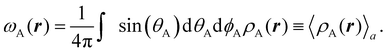
Contrary to the previous case, the weights ωB(r) satisfying eqn (1) can all of them be simultanously non-zero in fuzzy partitions. In this way, every point r is shared to different extents by all the atoms in the system. One of the possible choices of the ωB(r)'s was proposed by Axel Becke,48 just to facilitate the 3D integration of the one-electron functions that appear in Density Functional Theory (DFT). Indeed, any integral  is exactly given by a sum of atomic contributions
  as long as FB(r) = ωB(r)F(r), and the ωB(r) weights satisfy eqn (1). If F(r) = ρ(r) this procedure divides the total electron density into atomic densities.
In his original proposal, Becke defined the ωB(r)'s by dividing the space into fuzzy Voronoi polyedra that take into account the different atomic sizes through tabulated atomic radii. If, for the time being, we assume that all atoms are equal in size, the classical Voronoi cell of an atom A can be defined as follows. For the pair of atoms A and B, the elliptical coordinate μAB = (rA − rB)/RAB is defined, where rA and rB are the distances from nuclei A or B to a given point in space, and RAB is the distance between both nuclei. Any point r in the plane that bisects this line has μAB = 0. If the step function s(μAB) is defined as s(μAB) = 1 when −1 ≤ μAB ≤ 0 and s(μAB) = 0 when 0 < μAB ≤ +1, the Voronoi cell of atom A is given by a weight PA(r) = ΠB≠As(μAB), i.e. a point in R3 with PA = 1 belongs to atom A, otherwise it belongs to a different atom. The above definition provides a non-fuzzy partition of R3. However, a redefiniton of μAB in such a way that s(μAB) does not change abruptly from 1 to 0 in going from A to B allows for a fuzzy generalization of the partition. Becke's choice is 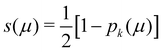 with pk(μ) = p(pk−1(μ)) and p1(μ) = (3/2)μ − (1/2)μ3. A small value of k, say k = 1, gives a slow decrease of s(μ) as we move away from the nucleus A, and k → ∞ provides again the original exhaustive partition. In general, the choice k = 3 is close to optimal and quite appropriate. The equal-atomic-size Becke's partition of R3 ends by defining
  through stockholder sharing, which automatically satisfies eqn (1). To account for the different atomic sizes, Becke replaces μAB by a new coordinate νAB = μAB + aAB(1 − μAB2) in the definition of pk, where |aAB| ≤ 1/2. The plane that bisects the AB internuclear axis in the original recipe is displaced towards center A or towards center B for positive or negatives values of aAB, respectively. Requiring that any point located in that plane (i.e. with νAB = 0) has rA/rB = RA/RB, where RA and RB are Bragg–Slater radii of both atoms, leads to aAB = uAB/(uAB2 − 1), where uAB = (χAB − 1)/(χAB + 1) and χAB = RA/RB. When aAB falls outside the |aAB| ≤ 1/2 range, Becke simply assigns the corresponding endpoint value to it.
Becke's partition method has been improved over the years to avoid some of its weak points. For instance, the atomic radii RA used in the definition of νAB can be determined on the fly and not from a tabulated list of values. When two atoms A and B are bonded according to QTAIM, RA and RB can be obtained from the distance of the BCP to both nuclei. If there is no a BCP point between A and B, the original recipe can be used.14 This choice leads to a modified Becke's method whose behavior is close to that of the exhaustive QTAIM partition. Another improvement is to change the definition of νAB, by using49νAB = (1 + μAB − χAB(1 − μAB))/(1 + μAB + χAB(1 − μAB)), which automatically takes into account the possible values of aAB greater than 1/2 or smaller than −1/2. This situation is not so uncommon and often happens when A and B have very different sizes. The above scheme, implemented by Salvador and Ramos-Córdoba,49 has been named topological fuzzy Voronoi cell (TFVC) partition by the authors. In an attempt to the TFVC partition to provide atomic electron populations as similar as possible to the QTAIM values, they choose k = 4, which does not imply an appreciable loss of precision of the numerical integrations that are necessary. Voronoi atoms have also been used by Fonseca Guerra and coworkers as a way to define the so-called Voronoi deformation density (VDD) charges.50 Among their many applications, they have been used to unravel a number of reaction mechanisms and bonding types.51,52
As a last variant of Becke's partition, it is worth mentioning about the proposal by Köster et al.53 These authors point out that the computation of the ωB(r)'s in the original algorithm grows with the third power of the number of atoms, which means that their calculation can be computationally very expensive. To remedy this they employed a modification of the atomic weight functions proposed by R. E. Stratmann et al.54 that involves replacing the p1(μ) expression used by Becke by another functions q1(μ;a), defined as q1(μ;a) = −1, q1(μ;a) = (3/2)(μ/a) − (1/2)(μ/a)3, and q1(μ;a) = +1 for μ ≤ −a, −a < μ < a and μ ≥ a, respectively. Moreover, they iterate this function three times to arrive finally at the function  , which is the analogous to Becke's s(μ) function. Köster et al. choose a = 0.7. The different definition of q1 depending on the value of μ dramatically reduces the CPU time required to construct the integration grids.
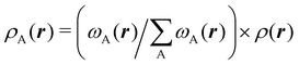
We stress that both Becke and Voronoi-like decompositions are geometric constructions lacking physical meaning. Their usefulness lies in their computational efficiency, or, as in TCFV, in its resemblance to other physically rooted decompositions, like that provided by the QTAIM. A radically different way of dividing the real space into fuzzy atoms is the one proposed by Hirshfeld as soon as in 1977.55 In order to carry out a population analysis in molecules, Hirshfeld introduced the reasonable idea that, at each point in space, the ratio between the density of one of the atoms (ρA(r)) and the total electron density (ρ(r)) should be the same as the ratio between the atomic density of the isolated atom A (ρ0A(r)) and the so-called promolecular density  . In other words
| |  | (2) |
The
ρ0A(
r)'s are usually taken as the spherically averaged atomic densities of neutral atoms.
An outstanding virtue of the atomic densities defined by eqn (2) is that they minimize the Kullback–Leibler entropy deficiency functional,56 defined by  so that these ρA(r)'s best preserve the information contained in the reference ρ0A(r)'s. This property places Hirshfeld's and related atoms among the very limited category of atoms-in-the-molecule that satisfy the physical properties or mathematical constraints. We refer the reader to the works of R. Nalewajski regarding the information on theoric treatment of chemical bonding.57 The original Hirshfeld partition exhibits some clear deficiencies. One of them is the strong dependence of the final electron population of the atoms-in-the-molecule (AIM) on the densities of isolated atoms, which is given by
  . For instance, the
 ![[n with combining macron]](https://www.rsc.org/images/entities/i_char_006e_0304.gif) Na and Cl values in the NaCl molecule, when the neutral
Na and Cl values in the NaCl molecule, when the neutral  and
and  densities of the isolated atoms are used to construct ρ0(r), are very different from those obtained when the ionic references
  and
and  are employed. In the first case, the net charges qNa = ZNa − Na and qCl = ZCl − Cl are too small, and far from the values obtained when
  and
and  are used in the method. It seems that Hirshfeld's original method tends to provide atomic charges close to those of the isolated atomic densities, and hence it does not account properly for ionic interactions.
There are several recent proposals aimed at improving Hirshfeld's original method. For instance, Bultinck et al.,58 in an attempt to minimize the strong dependence of the values of the A's on the atomic densities of isolated atoms, proposed the iterative Hirshfeld partition (Hirshfeld-I). As in the original method, the starting point (iteration zero) is computing the ωA(r)'s given in eqn (2) from some reference atomic densities ρ(0)A(r)'s. Let us call these initial weights ω(0)A(r). They are customary taken as the atomic densities of the isolated neutral atoms, although it has been proven that the final results do not depend on this choice. Next, the net charges of the atoms are computed as  . If qA ≥ 0, a new reference atomic density for A is obtained as
  where λ = qA − [qA] and [qA] stands for the integer part of qA. This procedure is nothing but taking the new reference atomic density for atom A as equal to the interpolated value between the isolated densities of ions with net charges [qA] and [qA] + 1. An analogous recipe is used in case that qA < 0. Then, improved weight functions
 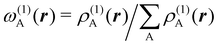 are obtained, and from them new net charges as
  in an iterative process that converges when the qA's in two successive cycles are less than a threshold value. A fast iterative procedure has been developed,59 based on Newton's method, which allows the convergence of the process to be achieved in very few cycles (normally, less than 10). An important point of Hirshfeld-I method is that the final atomic densities ρA(r) yield total electron populations of the atoms-in-the-molecule similar to those provided by the atomic references used to calculate the ωA(r) weights of the last cycle. Better variants that try to improve on still present caveats have also been published, like in the variational Hirshfeld method proposed by Heidar-Zadeh and coworkers.60 We will not extend here any more discussing the progressive improvements of Hirshfeld's method. For further information, we refer the reader to ref. 60. We notice that close to fifty years after Hirshfeld's original idea, the literature is riddled with a number of modified Hirshfeld rules that make it difficult for a non-expert to choose among them. This should be contrasted with QTAIM atoms, that have remained constant over that period of time.
Another procedure to obtain atomic densities ρA(r), very similar in spirit to the one just discussed, although formally different in its implementation is the iterative stockholder partitioning.61 Contrary to Hirshfeld-like methods, it does not require any calculation of the atomic densities of isolated atoms. It starts assuming ωA(r)'s equal to 1 for all the atoms. Then, initial atomic densities are obtained by using
| |  | (3) |
These atomic densities are then spherically averaged around their respective nuclei and taken as the next generation of atomic weights,
| |  | (4) |
The above integration is performed numerically and
r refers to the absolute position of an electron. The integral itself, however, depends only on
rA, the distance from nucleus A to the point
r.
Eqn (3) and (4) are applied until convergence.
All the partitions discussed so far, and also several unreported variants of them, require numerical integrations. In the case of Becke-like partitions, the method was designed to recover a global expectation value (typically, the exchange–correlation energy) by adding up all the atomic components. Many algorithms have been published to perform such integrations, but describing them is beyond the scope of this paper. We only want to point out that they can be grouped into two large families: those used for exhaustive partitions of R3 (typically, although not exclusively, the QTAIM partition) and those specifically focused on space partitions in fuzzy atoms.
To conclude this subsection, we must finally mention some other procedures that, albeit not strictly being atomic partitions of real space, have been widely used over the years, or are relevant to this particular work. Of course, it is mandatory to mention Mulliken's partition, used almost exclusively in the context of population analyses, and conventionally defined by 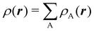 with
with  , where the ϕ's are nucleus-centered primitive functions, ρij are density matrix elements, and ρAij = ρij, ρAij = 0 or ρAij = (1/2)ρij when both ϕi and ϕj, none of them, or only one of them (ϕi or ϕj) are centered at nucleus A, respectively. Formally similar to Mulliken's atoms are the minimal deformation atoms defined by Fernández-Rico et al.,62 called deformed atoms-in-molecules (DAM) by these authors. They are determined by requiring that each bicentric contributions to ρ(r) has a minimal deformation. In the end, this criterion leads also to
  and
and  where ρAij takes the same values as in Mulliken's atoms, except when only ϕi or ϕj is centered at A, in which case ρAij = ρij if the function centered at A is the one with the largest exponent, and zero otherwise.
A comparison between the ωA weights for the C and O atoms of the CO molecule in some of the partitions discussed so far is found in Fig. 1 (mod-H is a variant of the Hirshfeld partition that has not been discussed here). As we can see, TFVC with k = 3 is the only case for which ωC = ωO = 0.5 at the BCP (denoted by a solid vertical line at about 0.66a0). At this point the QTAIM weight for the C (O) atom changes abruptly from 1 (0) to 0 (1). Although the figure illustrates the behavior of ωC and ωO only along the internuclear axis, it seems clear how the resemblance between the QTAIM and TFVC partitions increases as k grows.
 |
| | Fig. 1 Hartree-Fock (HF) TZV(2p,3d)++ atomic weight functions ωA(r) for carbon (A![[double bond, length as m-dash]](https://www.rsc.org/images/entities/char_e001.gif) C) and oxygen (AO) atoms of the CO molecule along the internuclear axis. C and O nuclei are at the −0.0424 and −2.0424 positions along the C–O axis, respectively. Labels Becke, TFVC (k = 3), and DAM stand for the original Becke's partition with Bragg–Slater radii, the modified Becke's partition with topological atoms, defined in the text as topological fuzzy Voronoi cell (TFVC) partition, and the deformed atoms in molecules (DAM) by Fernández-Rico et al., respectively. mod-H refers to a modified Hirshfeld partition not described in the text. Reprinted with permission from J. Chem. Theory Comput., 2006, 2, 90–102. Copyright 2006 American Chemical Society. C) and oxygen (AO) atoms of the CO molecule along the internuclear axis. C and O nuclei are at the −0.0424 and −2.0424 positions along the C–O axis, respectively. Labels Becke, TFVC (k = 3), and DAM stand for the original Becke's partition with Bragg–Slater radii, the modified Becke's partition with topological atoms, defined in the text as topological fuzzy Voronoi cell (TFVC) partition, and the deformed atoms in molecules (DAM) by Fernández-Rico et al., respectively. mod-H refers to a modified Hirshfeld partition not described in the text. Reprinted with permission from J. Chem. Theory Comput., 2006, 2, 90–102. Copyright 2006 American Chemical Society. | |
An important difference between fuzzy and non-fuzzy atoms is illustrated in Fig. 2, where we have lotted the atomic density of the left-H atom of the H2 molecule in four different partitions. We can see that the DAM density considerably invades the right part of the figure, that belongs in the QTAIM partition to the right-H atom. To a lesser extent, this situation also happens in the other two fuzzy partitions of the figure (Becke and mod-H). This behavior of overlapping atomic densities is general: fuzzy atoms display appreciable values in areas that, according to the QTAIM exhaustive partition, should be associated with other atomic moieties. Although orbital interpenetration is at the core of chemical thinking, fuzzy atoms seem to be less suitable than non-fuzzy ones as chemical bonding issues are regarded.14
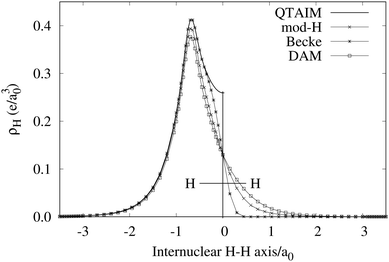 |
| | Fig. 2 CAS[2,2]/6-311G(p) atomic density for the left H atom of H2 along the internuclear axis. Left and right H atoms are at −0.7 and +0.7a0, respectively. Labels Becke and DAM have been defined in the text. mod-H refers to a modified Hirshfeld partition not described in the text. CAS[n,m] stands for a complete active space calculation with n electrons in m spin–orbitals. Reprinted with permission from J. Chem. Theory Comput., 2006, 2, 90–102. Copyright 2006 American Chemical Society. | |
3 The two faces of bonding: electron counting and energy decomposition
Once a suitable decomposition of a molecular system into atoms has been chosen, i.e., once a set of atomic weights ωA has been adopted, all expectation values can be partitioned into domain contributions. In order to simplify as much as possible, we will only consider spin independent operators in what follows. Let us take a general symmetric n-electron operator| | 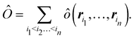 | (5) |
The structure of this expression includes, for instance, both the kinetic energy,  as well as the interelectron repulsion
  operators. Defining the nth order reduced density matrix (nRDM) (in McWeeny's normalization convention),63 as
| |  | (6) |
where we have abbreviated spin-spatial coordinate xi as i, and then the expectation value of operator Ô is given by| |  | (7) |
As it is customarily done, in this last expression, the operator acts on unprimed coordinates, after which the primed coordinates are equated to the unprimed ones before integration. Partitioning now the position of each electron into atomic regions, i.e. introducing a  term for each electron coordinate, we arrive at a general atomic partition of 〈O〉:
| |  | (8) |
where  .
.
In this way, the expectation value of any one-electron operator will become a sum of atomic components, that of a two-electron operator a sum of pairwise additive interatomic terms, etc. Typically, but not necessarily, it is the expectation value of the density matrices themselves as well as of the Hamiltonian of the system that are decomposed into atomic contributions. In the first case we come to the electron counting perspective of chemical bonding that divides the number of electrons or electron tuples (pairs, trios, etc.) in an atomic-wise manner. Taken to the limit, when each of the N electrons is integrated over some atomic domain, we come to the probability of finding a given partition of the electrons into the m nuclei of the system, what it has been called an electron distribution function (see below).64 If the one particle density (the diagonal 1RDM) or the electron density (ρ or 1RD) are integrated, we arrive at a population analysis. Similarly, if the pair density (the 2RD) is integrated over two different atomic regions, we get the number of electron pairs between them, NAB, a figure that can be compared to the product of the average electron populations, NA × NB.65 This product would provide the number of pairs if the electron populations of the two centers would be statistically independent. The difference NAB − NANB is thus a measure of the number of pairs shared between the atoms, a quantity that chemists associate with Lewis pairs and with bond orders. Note that this is actually a covariance. Descriptors based on the fluctuation of electron populations lie at the heart of the success of electron counting rules, and can be accessed through the so-called cumulant density matrices (CDMs).
In this regard, Mayer66 defined a bond order that takes into account the fact that, for atoms which interact with each other, the expectation value 〈![[N with combining circumflex]](https://www.rsc.org/images/entities/i_char_004e_0302.gif) AB〉 differs from the product 〈A〉 × 〈b〉, where A and B are the atomic electron population operators of atoms A and B, respectively. By using a second quantization formalism for non-orthogonal orbitals, he obtained δAB = −2[〈AB〉 − 〈A〉 × 〈B〉]. Shortly after, Giambiagi et al.67 rewrote Mayer's expression in the equivalent form δAB = −2 〈(A − 〈A〉) × (B − 〈B〉)〉, which gives the bond order a clear statistical interpretation, as it measures the correlation between the charge fluctuations on the individual atoms, vanishing when the motions of the electrons in A are independent from the motions of the electrons in B. Some years later, Angyan et al.68 made a comparison between two possible definitions of the bond order: the one derived from the exchange part of the two-particle density matrix and the other expressed as the covariance of the number of electrons between the atomic centers. Both definitions lead to identical formulae, although they predict different δAB's for correlated wavefunctions, as a consequence of excluding the correlation component of the two-particle density matrix. Actually, the fluctuation-based definition of the bond order had alreay been proposed in the seventies by Julg and Julg.69
AB〉 differs from the product 〈A〉 × 〈b〉, where A and B are the atomic electron population operators of atoms A and B, respectively. By using a second quantization formalism for non-orthogonal orbitals, he obtained δAB = −2[〈AB〉 − 〈A〉 × 〈B〉]. Shortly after, Giambiagi et al.67 rewrote Mayer's expression in the equivalent form δAB = −2 〈(A − 〈A〉) × (B − 〈B〉)〉, which gives the bond order a clear statistical interpretation, as it measures the correlation between the charge fluctuations on the individual atoms, vanishing when the motions of the electrons in A are independent from the motions of the electrons in B. Some years later, Angyan et al.68 made a comparison between two possible definitions of the bond order: the one derived from the exchange part of the two-particle density matrix and the other expressed as the covariance of the number of electrons between the atomic centers. Both definitions lead to identical formulae, although they predict different δAB's for correlated wavefunctions, as a consequence of excluding the correlation component of the two-particle density matrix. Actually, the fluctuation-based definition of the bond order had alreay been proposed in the seventies by Julg and Julg.69
If, in contrast, it is the Hamiltonian Ĥ that is partitioned, we arrive at a decomposition of the total energy in real space. Provided that the standard Coulomb Hamiltonian contains both one-electron (e.g. the kinetic energy and electron–nucleus attraction) as well as two-electron operators like the interelectron repulsion, the total energy will be written as a sum of intra- and inter-atomic terms. Separating these two types of contributions is the origin of the interacting quantum atoms (IQA) approach,14,70 which is probably the only orbital invariant energy decomposition scheme available at this time. As the only non-local operator in Ĥ is the kinetic energy, the only RDMs needed to perform an IQA decomposition are the non-diagonal 1RDM and the diagonal 2RDM.
We notice that, save the kinetic energy, which is a non-multiplicative operator that modifies non-trivially the 1RDM on which it acts, both the electron–nucleus and electron–electron interactions behave as distance-scaled RDMs. Thus, a close relationship between electron-counting descriptors, which depend on domain-averaged RDMs, and some IQA energetic terms exists. This provides a formal justification of the well-known bond-order bond-energy (BEBO) relationships.71
3.1 Cumulant densities and density matrices
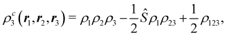
The nth-order cumulant density matrix (nCDM),72ρcn, is obtained after extracting from the nRDM, ρn, all those components that can be expressed in terms of RDMs of orders lower than n. If the same procedure is done with the diagonal components or reduced densities (RDs), the so-called cumulant densities (nCDs) are obtained. nCDs and nCDMs contain information about the n-electron correlations in the system. As Paul Ziesche73 has shown, these objects are actually the generators of the n-particle fluctuations of the electron distribution. In this sense, nCDs are intimately linked to the previously commented electron distribution functions,64,74,75 see below. Expressions for several cumulants can be found in ref. 76. The first, second and third order ones are, respectively,| | | ρc2(r1,r2) = ρ1(r1)ρ1(r2) − ρ2(r1,r2), | (10) |
| |  | (11) |
where Ŝρ1ρ23 = ρ1ρ23 + ρ2ρ13 + ρ3ρ12 are symmetrized products, and ρi, ρij, and ρijk are abbreviations for ρ1(ri), ρ2(ri,rj), and ρ3(ri,rj,rk), respectively. The first order cumulant density is just the electron density, and the second order one coincides with the so-called exchange–correlation density, ρxc2, which is immediately related to the McWeeny's exchange–correlation hole:| |  | (12) |
that measures the difference between the (conditional) probability density of finding an electron at r2 when another is located at r1 and the unconditional one, i.e. how the presence of an electron at r1 influences another at r2. Note that the hole integrates to one electron while the exchange–correlation density integrates to the total number of electrons in the system, N.
A relevant feature of nCDs is their extensivity, which allows ρcn−1 to be obtained from ρcn by integrating out the nth electron:
| |  | (13) |
If we recursively apply this relation to electrons
n,
n − 1,…, 1 we obtain
| |  | (14) |
Thus, a partition of any nCD into atomic contributions by integrating each of its electron coordinates over a given region provides a decomposition of the N electrons to which the cumulant integrates to, into atomic terms:
| |  | (15) |
The
NA1A2⋯An terms in the above expression, with all A
i's different, are
n-center generalizations of the
NAB two-center populations, and provide the number of electrons involved in
n-center fluctuations/delocalization/bonding. This provides the basis for introducing a hierarchy of electron counting techniques, which lead to the multicenter bonding indices initially introduced by Giambiagi, Bochicchio, Ponec, Bultinck, Matito, Solà and other authors.
77–80 We start by discussing electron counting issues, and move afterwards to energetic ones. The formalism of reduced density matrices of different orders as well as the
nCDMs, particularly the second order one, has been widely employed by Alcoba, Bochicchio, Lain, Torre, and others, in the analysis of local spins, the definition of several population analyses and covalent bond-order definitions, atomic valences, or the effectively unpaired electron density,
81–86 using both orbital-based (Mulliken) as well as topological partitions of space.
4 Electron counting
Armed with electrons as well as with energy partitioning, we will now consider how this general framework has been used to build insight into chemical bonding problems. Almost all the results that we will review have been obtained with the exhaustive QTAIM partition, although we stress that, as shown, the underlying methodology can be equally applied to any other partition.
4.1 Electron-number distribution functions
As explained in Section 3, any integral in which a given nRDM or nRD appears as part of the integrand can be appropriately partitioned into atomic (fuzzy or non-fuzzy) contributions. To put it bluntly, an arbitrary function F(r1,…,rN), where N is the number of electrons, can be expressed as a sum of mN contributions, being m the number of atoms of the system:| |  | (16) |
where| | | FB1⋯BN(r1,…,rN) = ωB1(r1)⋯ωBN(rN)F(r1,…,rN). | (17) |
Taking F(r1,…,rN) = 1, it is evident that, just as eqn (1) performs a partition of R3 into m domains, eqn (16) defines a partition of the 3N-dimensional space into mN regions. Suppose now that we have a normalized N-electron wavefunction Ψ that (for the time being) depends only on the spatial coordinates r1,…,rN, and take F(r1,…,rN) = Ψ*(r1,…,rN)Ψ(r1,…,rN), which is nothing but an scaled nRDM, then| |  | (18) |
Furthermore, assume that n1 values of the Bi's are equal to Ω1, n2 values are equal to Ω2,… and nm are equal to Ωm, with 0 ≤ ni ≤ N and n1 + ⋯ + nm = N. Since F(r1,…,rN) is symmetric with respect to the exchange of any two of the coordinates ri and rj, eqn (18) can then be re-written as| |  | (19) |
where N!Λ = N!/[n1! × ⋯ × nm!]. The number of terms in the summation is equal to NN,m = (N + m − 1)!/[N!(m − 1)!] that counts all the possible ways to choose the n1,…,nm set of electron counts such that their sum is equal to N. Similarly, the factor N!Λ simply counts the number of different possibilities of choosing the Bi fragments such that n1 of them coincide with Ω1, n2 with Ω2, and so on. Without any loss of generality it can be assumed that B1 = ⋯ = Bn1 = Ω1, Bn2+1 = ⋯ = Bn1+n2 = Ω2, and the last nm domains are equal to Ωm.
Eqn (19) is valid for fuzzy or non-fuzzy partitions of R3. However, in the latter case, where each ωB(r) is 0 or 1, it is customary to write it in the form
| |  | (20) |
where
D is an
N-dimensional domain in which the first
n1 electrons are integrated over Ω
1, the second
n2 electrons over Ω
2,… and the last
nm electrons over Ω
m. Remembering that
Ψ is normalized, each term of the above sum is the probability that
n1 electrons are found in Ω
1,
n2 electrons are found in Ω
2,… and
nm electrons are found in Ω
m| |  | (21) |
This statement simply arises from Born's interpretation of quantum mechanics. The set
S = (
n1,
n2,…,
nm) ≡ {
ni} defines a real space resonance structure (RSRS) and, from
eqn (20), the sum of all of them, as it should be, is equal to one:
| |  | (22) |
We have been assuming so far that each Ω
i identifies an
atom-in-the-molecule. However, the
ωi's of a subset of atoms can be added up to define fragment weight functions. This means that
m in all of the above can be identified with the total number of fragments in which we have grouped the atoms of the molecule. For instance, in methane (CH
4), we can define fragment 1 as the carbon atom and fragment 2 as the sum of the four hydrogen atoms. This gives
m = 2;
i.e. R3 = Ω
1 + Ω
2, with Ω
1 ≡ Ω = Ω
C and Ω
1 ≡ Ω′ = Ω
H1 + Ω
H2 + Ω
H3 + Ω
H4. In this and all two-fragment partitions of
R3, one has
S = (
n1,
n2) and, since
n1 +
n2 =
N, each RSRS is defined by just providing the number of electrons of one of the fragments; say
n1 ≡
n. Then,
eqn (21) can be written as
| |  | (23) |
Although
eqn (21) is not properly a probability when the space is divided into fuzzy atoms,
eqn (20) still holds in this case and, therefore, we will consider the former as a probability in what follows.
The wavefunction Ψ depends on the full set of electron coordinates x1,…,xN, where xi = r1 × σi is the product of a spatial coordinate (ri) and a spin variable (σi). Although the spin variables σi have not been included so far in our discussion, the generalization of eqn (21) to take them into account is easy:
| |  | (24) |
where we have replaced
F by |
Ψ|
2.
As written, eqn (24) does not state what the spin for each of the n1 electrons in Ω1, n2 electrons in Ω2, etc. is. If the N electrons are split in two subsets of Nα α and Nβ β electrons, with Nα + Nβ = N, a RSRS is defined now as S = (Sα;Sβ) ≡ {nα1,…,nαm;nβ1,…,nβm}, p(S) ≡ p(Sα;Sβ), and the probability that nα1 α electrons lie in Ω1, nα2 α in Ω2, etc., and nβm β electrons lie in Ωm, can be obtained by considering 2m domains, the first m with α spin and the last m with β spin. The result is
| |  | (25) |
where
Λσ = [
nσ1× ⋯ ×
nσm]
−1 and
σ = (α,β). Now,
D is a
N-dimensional domain such that the first
nα1 α electrons are integrated over Ω
1, the following
nα2 α electrons over Ω
1,… and the last
nβm β electrons over Ω
m. The set of all probabilities, {
p(
S)}, is called the electron number distribution function (EDF) of the system for the given partition. When the number of electrons of each spin in each domain is specified one speaks of a spin-resolved EDF. Otherwise, we have a spin-unresolved EDF. There are
NN,m = (
N +
m − 1)!/[
N!(
m − 1)!] and
NN,m =
NNα,m ×
NNβ,m = (
Nα +
m − 1)!/[
Nα!(
m − 1)!] × (
Nβ +
m − 1)!/[
Nβ!(
m − 1)!] probabilities in the spin-unresolved and spin-resolved EDFs, respectively. From their definition, it is notorious that the spin-resolved EDFs give a more detailed information than the spin-unresolved ones, and also that the latter can be obtained by adding the spin-resolved probabilities with a given value of
nα1 +
nβ1,
nα2 +
nβ2,…, and
nαm +
nβm.
Fast algorithms to compute the EDF in both cases, especially when the space is partitioned into not too many regions (say m ≤ 6) and the number of electrons is not too large (N ≤ 30), have been developed over the years. We refer the reader to the original references to learn more about them.64,75,87,88 For single-determinant wavefunctions (SDWs) there is no a priori difficulty (even for large N's) to calculate all the p(S)'s when the space is divided exclusively into two regions Ω + Ω′ = R3, as an explicit recursive formula was developed by Cancès et al.87 For m > 2, there is no explicit formula to compute the EDF. However, in many circumstances, several approximations endowed with a clear physical meaning can be used. Among these, we highlight the so-called core approximation. In the present context, it can be stated as follows: if from the set of molecular orbitals (used almost universally in the construction of Ψ) a number of them are almost entirely localized on one of the fragments, we can simultaneously increase by two (one α plus one β) the number of electrons of that fragment per localized orbital and exclude them from the calculation. In this way, we can reduce the effective value of N considerably and restrict the EDF calculation to the set of valence electrons.
It is customary in real space chemical bonding analyses to measure the degree of localization of a (normalized) molecular orbital (MO) ϕi(r) in a region Ω by the quantity 〈ϕi(r)|ϕi(r)〉Ω, i.e. the overlap of this MO with itself in that region. This is the diagonal element of the atomic overlap matrix (AOM), defined by
| |  | (26) |
This AOM definition holds for fuzzy and non-fuzzy partitions of space. The AOM integrals in all the domains Ω
1,…,Ω
m are the basic building blocks that one needs to compute the EDF in all cases (single- or multi-determinant wavefunctions (MDW), two (
m = 2) or more (
m > 2) fragments, …).
Extremely important for the analysis of chemical bonding by statistical analysis of EDFs is the fact that SDWs give rise to spin-resolved EDFs with α and β subsets of electrons that behave as statistically independent entities. This means that p(Sα;Sβ) is given by the direct product of the α and β EDFs
| | | p(Sα;Sβ) = pα(Sα) ⊗ pβ(Sβ). | (27) |
This is no longer true for MDWs. However, even in this case, there is a certain degree of α–β statistical independence which greatly facilitates the calculation of the spin-resolved EDF. When
Ψ is a MDW we can write it, in general, as
| |  | (28) |
where
cr are (variational or fixed-by-symmetry) coefficients and
ψr is a Slater determinant built with
N-spin orbitals
ϕr1,…,
ϕrN. When
Ψ in
eqn (25) is replaced by the above expression, the spin-resolved EDF results
89| |  | (29) |
where
| |  | (30) |
and it turns out that it can be written as the direct product of the corresponding components for both spins,
prs(
Sα;
Sβ) =
prsα(
Sα) ⊗
prsβ(
Sβ). Actually, the computational time required to perform this direct product is an important fraction of that needed to obtain the full EDF, especially when the total number of α and β probabilities is very high. In addition to the core approximation that we have already discussed, much computer time can also be saved by neglecting in
eqn (28) those determinants with coefficients
cr smaller (in absolute value) than a certain threshold value
εr, or those
rs terms in the sum 29 for which

where
εrs is another (small) threshold value.
Probabilities for single domains obtained through the Cancès fast algorithm87 have been widely used both using QTAIM and ELF basins.90 They have also been employed to define a new type of spatial partitioning in which general regions that maximize the probability of finding a given number of electrons are obtained through shape optimization techniques. These have been called maximum probability domains (MPDs),91 and have been examined in molecules92,93 in the mean-field regime, and also in solids.94 MPDs have great potential in the translation of chemical concepts, like the electron pair of Lewis, to the orbital invariant realm, but are notoriously difficult to compute and to generalize to the correlated regime.95 Some efforts to elucidate their properties and usefulness in the case of strong correlation have been made through the use of model Hamiltonians like that of Hubbard.96,97
4.1.1 Chemical bonding from the statistical analysis of EDFs.
Once the EDF of a molecule is available, it is possible to use it to obtain all kinds of statistical information about it. As an example, if all the m-fragment probabilities p(n1,n2,…,nm) are known, the marginal probabilities of having n1 electrons in Ω1, n2 electrons in Ω2,…, and nm−1 electrons in Ωm−1 irrespective of the value of nm are provided by| |  | (31) |
The one-fragment EDF can be obtained as| |  | (32) |
| |  | (33) |
We can obviously join several fragments into a single one, and add the probabilities in a different way. For instance, if the EDF for a partition R3 = Ω1 + Ω2 + Ω3 (i.e. m = 3) is known, and we join Ω1 and Ω2 into a new fragment Ω′ = Ω1∪Ω2, the p(n′,n3)'s are given by| |  | (34) |
In short, all the probabilities for a given partition are immediately accessible if those for a partition with a larger number of fragments are known.
Now, let us show how EDFs can provide valuable chemical bonding information. If we start from the one-center condensed probabilities, the pΩ(n) values for a given fragment Ω allow immediate recovery of its average electron population as  whose meaning is obvious: we simply multiply each possible value of the number of electrons in Ω(n) by its probability of occurrence (pΩ(n)) and carry out the sum for all ns. This value coincides with that obtained by integrating in R3 the density of the fragment,
| |  | (35) |
where
. The sum over A extends to all the atoms that belong to
Ω. In non-fuzzy partitions (in the QTAIM, for instance), the integral in
eqn (35) amounts to integrating the full density
ρ(
r) over the
Ω region:
| |  | (36) |
At this point we can immediately notice how the EDF expands our knowledge about the electron distribution. A standard population analysis will simply provide us with an average number of electrons for an atom. With the use of EDFs one clearly learns that the electron population fluctuates and that the average is made up of several electron counts with different probabilities of occurrence. Once this is understood, the relevance of knowing the width of this atomic electron count distribution becomes clear. If the width is very small, the atom will display a very sharp distribution of its number of electrons. We say that its electrons are localized. If, in contrast, the width (variance) is large, these electrons must be necessarily delocalized. Where? The covariance of a two-atom joint distribution will inform us about this. Actually, the cumulants of the EDF are immediately connected with those of the nRDMs.
73,98
For instance, just as 〈nΩ〉 can be obtained from the EDF or from ρ(r) (eqn (35) and (36)), the average 〈nAnB〉, where A and B are any two atoms of the system, can be computed in two different ways:
| |  | (37) |
where
ρAB2(
r1,
r2) =
ωA(
r1)
ωB(
r2)
ρ2(
r1,
r2). The covariance 〈
nAnB〉 − 〈
nA〉〈
nB〉 = 〈(
nA −
NA)(
nB −
NB)〉 (with
NA ≡ 〈
nA〉 and
NB ≡ 〈
nB〉) is a measure of the statistical independence between the two atoms. Note that this is the difference
NAB −
NANB commented above. In the QTAIM, a scaled value of this fluctuation is called the delocalization index (DI)
δAB![[thin space (1/6-em)]](https://www.rsc.org/images/entities/char_2009.gif) 99,100
99,100| | | δAB = −2cov(nA,nB) = −2〈(nA − NA)(nB − NB)〉, or | (38) |
| |  | (39) |
Thus, the second order cumulant of the probability distribution function is directly related to the atomic-condensed integral of the second order cumulant density. Similar, albeit more cumbersome, relationships exist between the
nth order cumulant of the EDFs and integrals of the
nCDs, which are used to define multicenter bond orders.
78 We note in passing that electron population fluctuations in spatial domains have been used many times in the literature to quantify electron localization and delocalization.
101,102 It is the fine-grained nature of the EDFs that provides a new look at their intimate nature.
When the electron populations of A and B are independent of each other, one has p(nA,nB) = p(nA) × p(nB), and then cov(nA,nB) = 0, and δAB = 0. δAB is customarily associated with the bond order between A and B, since it is easy to show that when the AOMs are condensed a là Mulliken, it coincides with the Wiberg–Mayer103,104 bond order. It is also closely related to the covalent interaction energy between both atoms. In a two-center molecule AB, the DI is positive definite, since an increase in the number of electrons in A (nA) is accompanied by a decrease in nB, and vice versa. In molecules with more than two atoms, this is not necessarily the case. There are situations (especially, but not only, in excited electronic states), which can be described as exotic, in which an increase in the population of one atom (say A) leads to an increase in the population of another (say B). This gives rise to positive covariances between both atoms and, consequently, to negative DIs.105 As a collorarly, the bond order thus measures the statistical dependence of electron populations in two atoms. Similarly, a multicenter bond thus only exist if there is mutual interdependence among the electron populations of more than two atoms.
As pointed out δAB ≥ 0 in diatomic molecules. However, the limit case δAB = 0 can only occur when there is a single p(nA,nB) ≠ 0 in the molecular EDF. This behaviour can be found, for instance, in the dissociation limit (RAB → ∞) of the ground state of dihydrogen, where the only resonance structure with non-zero probability is that with one electron in each atom. However, one can also show that at the Hartree–Fock (HF) level, δAB does not vanish at dissociation. At this level of theory, the wavefunction of H2 = HA − HB at any inter-nuclear distante RAB is given by the Ψ = |σg![[small sigma, Greek, macron]](https://www.rsc.org/images/entities/i_char_e0d2.gif) g| and the α and β electrons are statistically independent. The probability that the α electron be found in atoms A and B is the same, by symmetry, and equal to
g| and the α and β electrons are statistically independent. The probability that the α electron be found in atoms A and B is the same, by symmetry, and equal to  and the same happens with the β electron,
  . According to eqn (27), the spin-resolved EDF consists of four equal probabilities; namely
  . The sum of the first two is the spinless probability of finding one electron in A and the other in B (p(1,1)), regardless of their spin, and the third and fourth are the probabilities of finding both electrons in A (p(2,0)) and B (p(0,2)), respectively. Eqn (35) correctly predicts that each atom has on average one electron, 〈nA〉 = 〈nB〉 = 1. However, eqn (38) gives δAB = 1 at any RAB, which is clearly wrong and highlights the well-known dissociation problem of the Hartree–Fock model when the two resulting fragments are open shells. A minimum of two determinants are necessary to correctly dissociate dihydrogen. A complete active space calculation with two electrons in two spin–orbitals (CAS[2,2]), with wavefunction Ψ = c1|σgg| + c2|σuu|, where c1 and c2 are variational coefficients, remedies the problem and results in δAB values very close to those of a full configuration interaction (full-CI) calculation.98
At the equilibrium geometry, the mixing between the |σgg| and |σuu| configurations in the CAS[2,2] wavefunction of dihydrogen increases p(1,1) from 0.5 in the single-determinant (SD) calculation to about 0.58, and decreases p(2,0) = p(0,2) to 0.21. This behaviour can be easily rationalized (see below), and is quite general. In homonuclear diatomic molecules, electron correlation tends to narrow the distribution of probabilities around its neutral atom (NA = NB = N/2) value, and this results in a decrease of δAB. Actually, in the particular case of dihydrogen, it is trivial to prove from eqn (38) and the equality p(2,0) = p(0,2) that δAB = 4p(2,0) = 4p(0,2), so that the DI obviously decreases with increasing p(1,1) since p(1,1) = 1 −p(2,0) −p(0,2). This result can be corroborated in Table 1, which contains the EDF in dihydrogen as obtained with different methods. Notice how badly the Mulliken probabilities behave.
Table 1 CAS[2,2] EDF for H2 using different space partitions. Reprinted with permission from Springer Nature Customer Service Centre Gmb: Springer Nature, Theoretical Chemistry Accounts, generalized electron number distribution functions: real space versus orbital space descriptions, E. Francisco et al., 2010
| EDF |
p(2,0) = p(0,2) |
p(1,1) |
δ
AB
|
| QTAIM |
0.2083 |
0.5833 |
0.8332 |
| Becke |
0.2126 |
0.5749 |
0.8502 |
| Hirshfeld |
0.2299 |
0.5402 |
0.9196 |
| Mulliken |
0.1365 |
0.7270 |
0.5460 |
| Löwdin |
0.2255 |
0.5490 |
0.9019 |
| DAM |
0.1561 |
0.6877 |
0.6245 |
Another example of the decrease in δAB as the width of the distribution decreases can be seen in Fig. 3, where we have plotted the HF and CAS[10,8] p(nA,nB) values for several fuzzy partitions of space, as well as in the QTAIM partition, all for the N2 molecule. Only non-negligible probabilities (nA ≥ 4 or nB ≤ 10) are included in the figure. We observe that the HF p(nA,nB)'s are very similar in all the partitions, but differ considerably more in the correlated calculations (except p(6,8), which is very similar in all the cases). If, in a simple way, we estimate the width of the distribution by the value of p(7,7), we would conclude that, according to our previous arguments, the correlated δAB's should decrease in the order Löwdin > Hirshfeld > Becke > QTAIM > Mulliken > DAM. As we can see in Table 2 this is what actually happens. The smaller differences between the HF δAB's is a consequence of the great similarity between the HF distributions in the different partitions that we have already commented on.
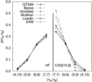 |
| | Fig. 3 Hartree-Fock and correlated EDF for N2 according to different space partitions. Reprinted with permission from Springer Nature Customer Service Centre Gmb: Springer Nature, Theoretical Chemistry Accounts, Generalized electron number distribution functions: real space versus orbital space descriptions, E. Francisco et al., 2010. | |
Table 2 Hartree–Fock and correlated CAS[10,8] p(7,7) values and delocalization indices, δAB, for the N2 molecule. Reprinted with permission from Springer Nature Customer Service Centre Gmb: Springer Nature, Theoretical Chemistry Accounts, generalized electron number distribution functions: real space versus orbital space descriptions, E. Francisco et al., 2010
|
|
HF |
CAS[10,8] |
|
p(7,7) |
δ
AB
|
p(7,7) |
δ
AB
|
| QTAIM |
0.3109 |
3.0408 |
0.3937 |
2.0113 |
| Becke |
0.3083 |
3.1073 |
0.3738 |
2.2298 |
| Hirshfeld |
0.2987 |
3.3664 |
0.3415 |
2.6879 |
| Mulliken |
0.3160 |
2.9110 |
0.4651 |
1.4618 |
| Löwdin |
0.2915 |
3.5613 |
0.3389 |
2.7703 |
| DAM |
0.3211 |
2.7834 |
0.5225 |
0.9998 |
4.2 Modeling EDFs
EDFs allow for an interesting classification of chemical bonds. Let us consider here only the two center case. The EDF for any two-electron system divided into two fragments A and B is fully characterized by p(2,0), p(1,1), and p(0,2), which can be collected in the vector| | | p2 = [p(2,0),p(1,1),p(0,2)]. | (40) |
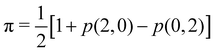
Since p(2,0) + p(1,1) + p(0,2) = 1, only two components of p2 are independent. As seen in the dihydrogen case, p(2,0) = p(0,2), with  or
or  for single- and multi-determinant descriptions, respectively. These results can be immediately extended to the SD case when both fragments are dissimilar. Let π and 1 − π be the probabilities that a first electron of an α–β electron pair is in A (p(A) = π) or B (p(B) = 1 − π), respectively. Since both electrons on a SDW are independent and indistinguishable, we will have p(2,0) = π2, p(0,2) = (1 − π)2, and p(1,1) = 2π(1 − π). To generalize these expressions to the correlated case, we can reason through a Bayesian analysis as follows.106 Provided that one of the electrons is in A, the probability that the second one is in B is
| | | p(B|A) = (1 + f)p(B) = (1 + f)(1 − π). | (41) |
Similarly, we have the following expression for the conditional probability that the second electron is in A if it is for sure that the first one is in B:| | | p(A|B) = (1 + f)p(A) = (1 + f)π. | (42) |
In eqn (41) and (42), f is a correlation factor whose value, necessarily in the range −1 ≤ f ≤ +1, measures how correlated the two electrons are. If f = 0, they are independent and p(B|A) = p(B), p(A|B) = p(A), i.e. the probability that one of the electrons lies in A or B does not depend on where the other electron is. Positive values of f imply that p(A|B) > π and p(B|A) > (1 − π). Both electrons are negatively correlated in this case and try to avoid each other: if the first one is in A(B), finding the second one in B(A) is more likely than if sites A(B) were empty. In contrast, if f < 0 we have p(A|B) < π and p(B|A) < (1 − π), and the presence of one of the electrons in A(B) increases the probability of finding the other in the same region: both electrons show a certain degree of bosonization.
The probability p(1,1) is given by
| | | p(1,1) = p(A|B)p(B) + p(B|A)p(A) = 2(1 + f)π(1 − π), | (43) |
with
p(A|B)
p(B) =
p(B|A)
p(A) due to electron indistinguishability. In the two limit cases
f = 1 and
f = −1,
p(1,1) = 4π(1 − π) and
p(1,1) = 0, respectively. If, in addition, we are in the non-polar case, we have
, and
p(1,1) = 1 for
f = 1.
When an electron is in A the other is necessarily in A or B, so that p(A|A) +p(B|A) = 1. Similarly p(A|B) +p(B|B) = 1. From these two expressions and eqn (41) and (42) one obtains p(A|A) = 1 − (1 + f)(1 − π) and p(B|B) = 1 − (1 + f)π. Finally, in addition to eqn (43) for p(1,1), we have
| | | p(2,0) = p(A)p(A|A) = π[1 − (1 + f)(1 − π)], | (44) |
| | | p(0,2) = p(B)p(B|B) = (1 − π)[1 − (1 + f)π]. | (45) |
p(2,0) and
p(0,2) can also be written as
p(2,0) = π
2 − π
f(1 − π) and
p(0,2) = (1 − π)
2 − π
f(1 − π), or
p(2,0) =
p(2,0)
indep − π
f(1 − π) and
p(0,2) =
p(0,2)
indep − π
f(1 − π);
i.e. the same quantity, equal to half the increase in
p(1,1) due to correlation effects, must be subtracted from their corresponding independent electron values. In the end, any vector
p2 is uniquely determined with two chemically relevant parameters, the net electron transfer towards site A given by
q = 2π − 1, and the correlation factor
f. These are easily inverted, since
f = {
p(1,1)/[2π(1 − π)]} − 1 and
.
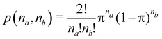
If each electron has a probability π ≡ SA of being in A and 1 −π ≡ SB = 1 − SA of being in B and both electrons are independent, the three components of p2 can be obtained from the binomial distribution106
| |  | (46) |
yielding
p(2,0) =
p(0,2) = 1/4 and
p(1,1) = 1/2 in the symmetric case (π = 1/2). In a heteropolar union, one of the two fragments is more likely to retain the electrons, and the polarity parameter π≠1/2. In the π = 0 or π = 1 limits,
p2 collapses onto
p2 = (0,0,1) and
p2 = (1,0,0), respectively. From
eqn (46),
p2 = [π
2,2π(1 − π),(1 − π)
2]. This is the general expression of
p2 for a (2c,2e) uncorrelated bond. A (2c,2e) bond with correlated electrons may be fully characterized from a Bayesian analysis of
p2 through the π parameter (or the net electron charge transfer towards fragment A,
q = 2π − 1) and a correlation factor
f =
p(1,1)/[2π(1 − π)] − 1,
106 which is the coarse-grained analogue of the standard
f in density matrix theory. This is evident if the above expression is written as
| | | p(1,1) = 2π(1 − π)(1 + f) = p(1,1)indep[1 + f], | (47) |
which is the analogue of equation
ρ2(
r1,
r2) =
ρ(
r1)
ρ(
r2)[1 +
f(
r1,
r2)] of density matrix theory. In this correlated case,
p(2,0) = π
2 − π(1 − π)
f and
p(0,2) = (1 − π)
2 − π(1 − π)
f.
The correlation factor f lies in the range −1 ≤ f ≤ +1, and cleanly classifies (2c,2e) links into three categories: (1) bonds with statistically independent electrons (f = 0); (ii) bonds with electrons that try to avoid each other (f > 0 or p(1,1) > p(1,1)indep) or normal bonds (NB); (iii) bonds with positively correlated electrons (f < 0 or p(1,1) < p(1,1)indep). These are related to the charge-shifted bonds (CSBs) in valence bond theory.107 Note that, usually, electrons are negatively correlated, so that they display positive correlation factors. Up to the moment of writing, bosonized states have only been found in excited states.105 Their electron distribution is so different from what chemists are used to that they promise to provide new insights into chemical bonding.
In the (q,f) polarity-correlation coordinates, the DI between A and B is δAB = 4(1 − f)π(1 − π) = (1 − f)(1 − q2). Thus, non-polar (π = 1/2) NBs (f > 0) give δAB = 1 − f < 1, and non-polar CSBs (f < 0) display δAB = 1 − f > 1, with the limits δAB = 0 and δAB = 2 when f = +1 or f = −1, respectively (thus, 0 ≤ δAB ≤ 2 in non-polar bonds). The p2 vector in these two limit cases is given by p2 = (0,1,0) and p2 = (1/2,0,1/2). p2 = (0,1,0) implies that, whenever one takes a picture of the system, one of the electrons lies in A and the other in B. That is, there is no electron sharing at all. In this case, interpreting δAB as a bond order is coherent. However, since p2 = (1/2,0,1/2) means that the two electrons are either both found in A or in B, using δAB as a bond order in strongly non-binomial EDFs with f ≃ −1 should be undertaken with care. In this case, the electron distribution does not resemble any textbook model, and chemical intuition, which is heavily based on them, fails. Note, however, that from the point of view of the fluctuation of electron populations, δAB has the same interpretation always.
Everything we have discussed in the last paragraphs is beautifully illustrated in the triangular graphical representation of Fig. 4, where all possible two-fragment two-electron EDFs are plotted in a ternary diagram. The evolution of the delocalization index, correlation factor or net charge transferred from one fragment A to the other B is clearly identified. Note how the area of normal bonds with positive f values is considerably smaller (actually one third of the full area of the triangle) than that corresponding to negative correlation factors. No diatomic molecule in its ground state has been found yet to populate the negative correlation factor region.
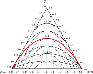 |
| | Fig. 4 Ternary representation of a two-fragment two-electron EDF. For any point inside the triangle, p(2,0), p(1,1), and p(0,2) are given by the distances from it to the left, bottom and right sides, respectively. Isolines of f from top (f = 1) to bottom (f = −1) are represented by full solid lines at intervals of 0.25. Dashed lines, tangent to f isolines at the p(2,0) = p(0,2) point, and growing from 0 (top) to 2 (bottom), in intervals of 0.25, are δAB isolines. Constants q isolines, growing from q = −1 (left) to q = +1 (right), at intervals of 0.2, are the vertical dashed green lines. The thick red solid line separates NBs (upper part) from CSBs (lower part). Reproduced from ref. 106 with permission from the Royal Society of Chemistry. | |
The generalization of the above ideas to more than a single bond has already been presented.106 The idea is to recover the full N-electron EDF, pN, in terms of the probabilities associated with a smaller number of electrons. Let us consider that the system has an even number of electrons (N = 2n), and assume that (a) the molecule is well described by a set of n = N/2 two-center, two electron (2c,2e) bonds, and (b) that all of these bonds are independent of each other. Then,
The direct product symbol (⊗) in the above equation simply takes this second assumption into account. We now assume that
pi2 = [
pi(2,0),
pi(1,1),
pi(0,2)], where
| | | pi(1,1) = πi(1 − πi)2(1 + fi), | (49) |
| | | pi(2,0) = πi2 − πi(1 −πi)fi, | (50) |
| | | pi(0,2) = (1 − πi)2 − πi(1 − πi)fi. | (51) |
In this way, the set {π
i,
fi} (
i = 1,
n) defines
pN. The better the hypotheses (a) and (b), the better
eqn (48) is fulfilled. The pair of atoms involved in each
pi2 can be equal or different. In the first case, one expects π
i to be close to ½. A value of π
i exactly equal to ½ can only occur if, in addition to both atoms being similar, they have a similar environment in the molecule. On the other hand, when the polarity of both atoms is different, π
i will deviate from its mean value, getting closer to 1 (0) when the atom A(B) is much more electronegative than B(A). The optimal set {π
i,
fi} can be determined by minimizing the quantity
δ, defined as
| | 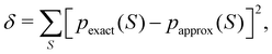 | (52) |
where
pexact(
S) are the exact probabilities and
papprox(
S) the approximated ones obtained by applying
eqn (48). To exploit the above fitting strategy in those cases where one believes that hypotheses (a) and (b) are reasonably accurate, the following steps are taken: (1) A given number of types of bonds is assumed and the initial values of π
i and
fi chosen, (2) each pair of atoms of the molecule is assigned zero, one, or more of the above types, and (3)
δ is minimized with respect to the {π
i,
fi} parameters.
A very simple example can be used to illustrate the procedure. Let us take a hypothetical molecule AB2 ≡ B1 − A − B2 and assume that a single (2c,2e) bond exists between the atom A and each of the two similar atoms B. Then, there exists only a type of bond and two optimizable quantities π1 = π2 = π and f1 = f2 = f. The vector pN consists of nine components p1(1,1)p2(1,1), p1(1,1)p2(2,0),…, p1(0,2)p2(0,2). Each of these products contributes to the probability papprox(nA,nB1,nB2) of a specific three-center four electrons RSRS. For example, p1(1,1)p2(1,1) adds to papprox(2,1,1), p1(1,1)p2(2,0) adds to papprox(3,1,0),…, and p1(0,2)p2(0,2) adds to papprox(0,0,4).
The presence in a molecule of lone or core electron pairs on one or more of the atoms also fits into the above scheme. For instance, in the trans-N2H2 molecule, we can reasonably assume that the 1s cores of nitrogen atoms are not involved in any bond. If we set πi = 1 and fi = 0 for one of these pairs, and fix their values, its effect on pN will be to increase the number of electrons in the corresponding atom by 2. Let us assume three types of bonds here, types 1 and 2 associated with the N–N pair, and type 3 to each N atom and the H atom closer to it. At the CAS[12,8]/6-311G(d,p) level of calculation, the results obtained after minimizing the δ quantity can be seen in Fig. 5 and Table 3. The agreement between the exact and fitted probabilities is very good. Only a few fitted p(S)'s deviate a little from the exact ones. As corresponds to two equivalent atoms in equivalent environments, the π value for both N–N bonds is very close to ½ (q ≃ 0.0), with correlation factors being strongly positive. This results in a p(1,1) probability much larger than p(2,0) = p(0,2) and a  much smaller than 1.0. The π value for the N–H bond is considerably larger than 0.5, which indicates a clear polarization towards the nitrogen atom, as it is evident if we compare the p(2,0) and p(0,2) values: if one takes an infinite number of snapshots of the N–H bond, 48% of the time both electrons will lie within the N region. The two electrons of these N–H bonds are positively correlated (fi < 0), although we suspect that the value of fi is not very significant in this case, and that it simply absorbs other electronic delocalizations that have not been taken into account in our simple bonding model. Finally, we should notice in the final part of Table 3 that the approximate δAB's are quite similar to the exact ones, particularly for N–H bonds. In the table, N2–H3 and N1–H4 refer to the hypothetical bonds between each N atom and the H atom farthest from it. The exact δAB for them are close to 0.0, which justifies that we have not assumed their existence in our model. The same happens with the hypothetical bond between the two H atoms.
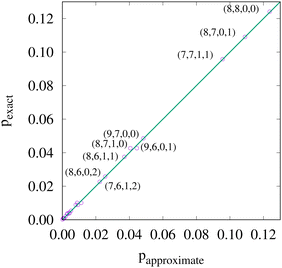 |
| | Fig. 5 Exact (y-axis) versus fitted (x-axis) EDF for N2H2 at the CAS[12,8]/6-311G(d,p) level of calculation. Only non-equivalent probabilities with pexact > 0.02 are labeled. The four integers on each label are the number of electrons in N1, N2, H1, and H2. | |
Table 3 Parameters of the EDF fitting of N2H2 molecule at the CAS[12,8]/6-311G(d,p) level of calculation. N1–H3 and N2–H4 are the standard polar N–H bonds, and N1–H4, N2–H3, and H3–H4 are non-bonded pairs
| Pair → |
N1–N2 |
N1–N2 |
N1–H3 |
N2–H4 |
|
q
|
0.000375 |
−0.000216 |
0.379834 |
0.379834 |
| π |
0.500187 |
0.499892 |
0.689917 |
0.689917 |
|
f
|
0.594557 |
0.260804 |
−0.015801 |
−0.015801 |
|
δ
AB
i
|
0.405443 |
0.739196 |
0.869247 |
0.869247 |
|
p(2,0) |
0.101548 |
0.184691 |
0.479365 |
0.479365 |
|
p(0,2) |
0.101173 |
0.184907 |
0.099532 |
0.099532 |
|
p(1,1) |
0.797279 |
0.630402 |
0.421103 |
0.421103 |
| Atom → |
N1 |
N2 |
H3 |
H4 |
| 〈nA〉exact |
7.375559 |
7.375307 |
0.624567 |
0.624567 |
| 〈nA〉approx |
7.379993 |
7.379675 |
0.620166 |
0.620166 |
| Pair → |
N1–N2 |
N1–H3 |
N2–H3 |
N1–H4 |
N2–H4 |
H3–H4 |
|
δ
AB (exact) |
1.077506 |
0.860953 |
0.032239 |
0.032262 |
0.860930 |
0.003975 |
|
δ
AB (approx) |
1.144639 |
0.869247 |
0.000000 |
0.000000 |
0.869247 |
0.000000 |
The δ error in the above example is quite small (0.000028). When this does not occur, it is very likely due to an inappropriate choice of the proposed bonding pattern. When it is almost certain that there are no (nc,2e) multicenter bonds (n > 2), a decrease of δ may be achieved by including other p2 vectors in eqn (48). If, even so, the value of δ does not decrease, the initial assumption that EDF can be represented as a direct product of (2c,2e) bonds is simply wrong, and alternative models that explicitly account for these forgotten (nc,2c) bonds should be developed. Although we will not pursue this objective in this work, some didactic examples are explained in some detail in ref. 98.
5 Energy decompositions
As stated in Section 3, the second face of chemical bonding is energetic. After all, no bonding exists without an energetic stabilization. This statement can be assessed with respect to some appropriately defined set of fragments that interact or, in the case of metastable bonds (like that in the O22+ cation, for instance108), with respect to some finite geometrical perturbation. When chemical insight is to be pursued it is clearly not sufficient to report the overall dissociation energy; chemists would like to know which fragments, bonds, or moieties are responsible for it and to what extent. This background leads necessarily to consider an energy decomposition scheme. Not unexpectedly, there are dozens, if not hundreds of them out in the literature. Very grossly speaking, three families of energy decomposition analyses (EDAs) have survived through the present time. In the case of weakly interacting systems, the traditional theory of intermolecular interactions that computes the interaction between two (or more) unperturbed fragments by means of perturbation theory has evolved into very accurate and complex methods, among which we highlight the well-known symmetry adapted perturbation theory (SAPT).109 SAPT and related perturbative approaches suffer from two very clear problems. On the one hand, they fail to converge easily in the short-range regime, so that a user never knows when the perturbation series stops being reliable. On the other hand, the use of unperturbed monomers fails to reflect the changes that their densities, orbitals, etc. experiment after the interaction has taken place. When a supermolecule is computed and compared to the interacting fragments, the original Morokuma decomposition,110,111 generalized by Ziegler and Rauk,112 has turned into a set of very useful recipes, frequently used in density functional calculations.113,114 This energy decomposition analysis depends heavily on how the fragments that interact are chosen, being thus reference dependent. Finally, if atoms are singled out from a molecule, another set of EDAs emerge which compute their energies and mutual interactions. This procedure can be done in orbital space, as for instance, in the methods proposed by Head-Gordon and coworkers,115 which also use some artificial states borrowing ideas from Morokuma-like partitions, and depend obviously on how atoms are extracted in orbital space. If done in real space, like in the interacting quantum atom (IQA) decomposition,70,116–119 no reference is needed at all, although the procedure now becomes dependent on how the real space atoms are defined. From a wavefunction, a consistent decomposition of the expectation value of the Hamiltonian into atomic and pairwise additive contributions is obtained. These ideas will be further discussed in the next subsection.
5.1 The IQA energy partition
Let us consider either a fuzzy or an exhaustive partition of space, as provided by a set of ωA weights (see Section 2). Once this has been chosen, the expectation value of the Hamiltonian can be written as:| |  | (53) |
wherein  and ρ2(r1,r2) are 1RDM and the 2RD, respectively, ĥ(r1) is the monoelectronic part of the electronic Hamiltonian as a function of the coordinates of electron 1, while r12 represents the distance between electrons 1 and 2 and Vnn is the internuclear repulsion. Finally, EAself and EABint represent the energy terms which contain particles (i) in only one basin A or (ii) in two different basins A and B, respectively, and are known as the atomic self-energy of atom A and the interaction energy between atoms A and B, respectively. Eqn (53) represents the basis of the Interacting Quantum Atom (IQA) energy partition.14,70
The atomic self-energy contains all those energy terms that would survive after full dissociation of the system into its atoms: the kinetic energy of the electrons, the electron-own nucleus attraction and their mutual repulsion:
| | | EAself = TA + VAAen + VAAen. | (54) |
As we progressively dissociate a molecule into its atomic components, all the atomic self-energies evolve to the
in vacuo atomic energies. An atom's self-energy is the local expectation value of the atomic Hamiltonian in-the-molecule. It is rather obvious that the magnitude of a given
EAself will be on the same scale as that of the
in vacuo energy of A. Namely, about −0.5
Eh for a hydrogen atom, around −100
Eh for a F moiety. This means that, although no reference is needed to perform an IQA decomposition, if a suitable atomic reference is chosen (
e.g. the evolved atomic states at dissociation) the energetic difference between the self-energy and this reference energy will be small, in the chemical scale, measuring the energy associated with the chemical deformation experienced by the atom on going from its reference to its in-the-molecule state. We call these differences deformation energies:
| | | EAdef = EAself − EA0, | (55) |
EA0 being the chosen reference energy for atom A. Deformation energies are typically positive, since it takes some energy to deform a free atom to get it bonded. Their values are chemically intuitive, in line with the traditional idea of valence excitation. For instance, since Li in LiF has almost lost one electron which has been taken by the very electronegative F atom, the in-the-molecule state of Li is largely cationic, so its self-energy will have been destabilized with respect to the neutral reference by about its ionization potential. Similarly, we expect that the deformation energy of fluorine in LiF to be small or even negative, since although the moiety needs to be deformed to get bonded, the atom will have also gained energy close to the electron affinity of F in the process. These intuitions are supported by actual calculations.
120
In a similar manner, the interatomic interaction energy between two atoms, EABint, contains all energetic components affecting mutual interaction of their electrons and nuclei: the attraction between the electrons on A and the nucleus of B and vice versa, the repulsion between the electrons lying in A and those lying in B, and the internuclear repulsion:
| | | EABint = VABen + VBAen + VABee + VABnn. | (56) |
In the large interatomic distance limit,
EABint provides exactly the interaction energy that is obtained from perturbation approaches. Nevertheless, an important difference is that
EABint, unlike perturbational methods, has a well-defined limit at any distance. The interaction energy can be chemically exploited by dividing the pair density
ρ2(
r1,
r2), into Coulombic and exchange–correlation terms, as in Eq. 10. If this is done,
EABint becomes a sum of a Coulombic term, which depends only on the 1RD,
i.e. on classical electrostatics from the quantum-mechanically obtained densities, and an exchange–correlation term, purely quantum-mechanical in origin:
| | | EABint = VABcl + VABxc. | (57) |
The first is clearly related to ionicity, while the second, which comes from integrating an interelectron distance-scaled, measures the energetic effect of electron fluctuation (or delocalization) and thus provides a direct connection with covalency. The interaction energy between two atoms is thus divided into a term that tends to the standard multipolar series at large interatomic distances, dominated by the fist non-zero atomic multipolar moments, and a contribution which does only exist due to quantum fluctuations. These ideas are chemically appealing and they have been documented in detail.
13
The IQA partition can be exploited at different levels of granularity, viz., it can be equally applied to groups of atoms  so that
| |  | (58) |
wherein
| |  | (59) |
and
| |  | (60) |
The interaction energy between two groups  can also be divided in Coulombic and exchange–correlation contributions,
  and
and  in a similar fashion to EABint in eqn (57). This ability of the IQA approach to provide chemically intuitive answers at different granularities allows for a relatively easy way to compare it to other energy decomposition methods. The other way around is not so obvious. We refer the reader to specific publications on the subject for further information.121,122
IQA can also be used in the multi-component MC-QTAIM formalism.47 This is a very promising strategy that may help understand how chemical bonding evolves when the Born–Oppenheimer approximation breaks and the quantum nature of nuclei needs to be considered. We refer the reader to the above reference for further details.
Although  and ρ2(r1,r2) are not attainable via Kohn-Sham Density Functional Theory (KS-DFT), it is possible to divide the KS-DFT electronic energies using scaling techniques as suggested in ref. 123 and 124. Taking into account the popularity of the KS-DFT in modern computational chemistry, this pragmatic strategy has reinforced the applicability and interest of IQA. However, the relatively-high computational cost of IQA is the major inconvenience that remains for its widespread use. This situation, which occurs because the IQA terms involve the integration of scalar fields over very irregular regions, is aggravated for correlated scalar fields
  and ρ2(r1;r2). We expect that such calculations could be accelerated by introducing carefully-controlled approximations, as found in the case of the partition of MP2 correlation energies using effective two-electron matrices,125 which reduces in ∼ 80% of the computational cost for double- and triple-ζ basis sets. More considerable reductions in computer time may result for larger basis sets.
5.2 Multifaceted applications of IQA
Chemists are often interested in the nature and the relative strength of covalent and noncovalent interactions under different circumstances. Indeed they characterize all kinds of interactions in terms of heuristic, intuitive chemical concepts such as steric hindrance, π-conjugation, aromaticity, cooperative and anticooperative effects, etc. Within this context, the IQA method can provide much valuable information, not only by assessing the energetic magnitude and essential features of chemical contacts in diverse scenarios, but also by providing quantitative descriptors of those concepts that are not associated with Dirac observables and thereby lack a rigorous mathematical definition. Thus, we will show that the applicability of the QTAIM and IQA methods is gradually expanding and, as recently noticed by Richter et al.,126 their additional computational effort is more than compensated by the great amount of useful information they provide. Several authors have used IQA to provide unified models of chemical bonding. In this sense, Cukrowski,127 has advocated for using fragments in his Fragment Attributed Molecular System Energy Change (FAMSEC) familiy of methods to solve a battery of chemically relevant problems.128–130
In this perspective, we will focus on the IQA analysis performed within the QTAIM framework although it can also be applied to other scalar fields such as the ELF partition.131–133 Let us discuss first the characterization of selected noncovalent complexes, which is no doubt one of the most typical goals of EDAs. In this regard, IQA has been successfully employed to explain the experimentally observed Hydrogen Bond (HB) cooperative effects in water clusters.134 For example, IQA has unveiled that double HB donors and acceptors of HB can also be associated with marked cooperative effects,135 in contrast with the traditional view that associates them with anticooperative effects.136 Likewise, the IQA partition puts forward a hierarchy of HB strength within water clusters as a function of the single/double and donor/acceptor character of the involved monomers.137 In general, IQA has proven useful to characterize the underlying classical and quantum-mechanical effects in other prototypical noncovalent interactions, such as the crucial role played by the exchange–correlation stabilization complementing the electrostatic picture of both anion–π138 and halogen bonding139,140 complexes.
Perhaps one of the major appealing features of IQA is the determination of the attractive or repulsive character of A⋯B or  interactions as well as their covalent and ionic contributions. For instance, the stabilizing role of the H⋯H interaction proposed by Matta and coworkers143 has been the subject of considerable debate.144,145 Several IQA studies146–148 have confirmed the attractive character of this interaction. In like manner, the IQA energy partition and other EDAs have been exploited to determine that the CH⋯HC interactions in the “in–in” conformation of ortho-xylene are also attractive.149 Therefore, the larger stability of the “out–out” conformer is due to other factors which include charge delocalization and aromaticity.
Let us consider in more detail another similar problem, the IQA assessment of the so-called Jørgensen Secondary Interaction Hypothesis (JSIH).141,142 The JSIH states that the relative strength of similar H-bond complexes can be determined by the balance between the attractive and repulsive interactions among the frontier atoms between the interacting monomers. For example, JSIH correctly predicts that amides dimerize more strongly than imides because imide dimerization is impaired by a repulsion that involves the oxygens of the spectator carbonyls (dashed arrows in Fig. 6(a)). Additionally, the JSIH rightly foretells that AAA–DDD complexes are stronger than those of the type AAD–DDA wherein A stands for HB acceptors and D for HB donors. In turn, AAD–DDA clusters are stronger than those of the sort ADA–DAD (Fig. 6(b)). Nevertheless, the JSIH wrongly foresees that the strength of amide–imide heterodimers should be intermediate between that of the corresponding homodimers (Fig. 6(c)). However, the IQA descriptors indicate that all the atoms within the monomers should be considered to properly account for the intermolecular formation energy (see for example atom C1 in Fig. 6(d)). Ref. 141 concludes that the relative strengths of homo- and hetero-dimers of amides and imides can be better explained by considering the acidity and the basicity of the involved HB donors and acceptors, respectively.
 |
| | Fig. 6 (a) and (b) Jorgensen Secondary Interaction Hypothesis (JSIH) applications to the study of hydrogen bonded systems. Solid/dashed arrows indicate JSIH attractions/repulsions between the interacting molecules. The JSIH predicts that (a) the amide homodimers are more strongly bound than imide homodimers and (b) the order of strength for complexes with hydrogen bond acceptors (A) and donors (D) is AAA-DDD > AAD-DDA > ADA-DAD. (c) Association constants and changes in chemical shift in CDCl3 at 25° of δ-valerolactam and 3,3-dimethylglutarimide. The heterodimer is more strongly bound than the two homodimers. (d) IQA energy partition for the dimerization of 3,3-dimethylglutarimide. One monomer and its atoms are indicated in green color. Ditto for the other monomer and orange color. The values are reported in kcal mol−1. Note that the interactions of C1 with the interacting monomer I are also important to the interaction between the two monomers. The deformation energies of the monomers are 16.4 and 20.0 kcal mol−1 so that the formation energy of the dimer is − 10.4 kcal mol−1. Adapted from ref. 141 and 142 with permission from the Royal Society of Chemistry. | |
As stated above, the QTAIM and IQA methods of wave function analysis contribute to the understanding of intuitive and heuristic chemical ideas. An intuitive chemical concept whose quantum mechanical foundation has been addressed by means of IQA is Sterical Hindrance (SH).150 For a given pair of frontier atoms A⋯B located in different molecules, their deformation energies EAdef and EBdef can be fitted to an exponential decaying function,151 which corresponds to the repulsive part of the Buckingham potential Urep ∼ exp(−αr).152 This observation has led to the proposal that EAdef + EBdef equals the short-range repulsion energy of these atoms, and that such repulsive interaction acts over distances longer than previously envisioned (other IQA studies153 predict a different behavior of the H atom in this regard). More recently, it has been pointed out154 that changes in the number of electrons have a very significant contribution in deformation energies. In other words, an assessment of the SH energetics would be biased by alterations in the electronic population of the atoms in a process under consideration. Hence, charge transfer energy should be subtracted from the deformation energy to yield a quantitative measure of the SH of atom A, that is, EASH = EAdef − EACT where EACT = EAref(N) − EAref(N0) estimates the charge transfer contribution when N and N0 are the electrons of A in its final and initial (reference) states, respectively. The suitability of the EASH expression has been validated in different archetypical systems such as atomic compression and SN2 reactions in which SH is usually invoked.
Clearly, the strengthening or weakening of chemical interactions under different scenarios as provided by IQA can be very useful to understand chemical reactivity, especially when the appropriate IQA descriptors are monitored along the process to determining which interactions or atoms are mostly responsible for the occurrence (or lack of) of a chemical reaction, what might result in directives for the tuning of chemical modifications in reactants. In addition the selection of group-based IQA quantities is normally required given that, besides the atoms involved directly in the bond forming/breaking, other contributions need to be considered in order to account for the net energy changes along the reaction profiles.155 For instance, the changes in the steric energy associated with reacting molecules (i.e.,  ) supports the kinetic role of SH that is traditionally claimed to play in the competition between SN2 and E2 reactions.156 On the other hand, the geometric and electronic deformation of a diene/dienophile helps to understand the origin of the endo–exo preference in prototypical Diels–Alder reactions157 while the atomic IQA decomposition of the IRC profiles explains the synchronous or asynchronous character of the polar Diels–Alder reactions.126 Focusing also on the proper fragment quantities, the IQA study of the bifunctional catalysis played by water clusters158 shows how water monomers encompassing the reaction between SO3 and H2O to yield H2SO4 mitigate the changes in chemical bonding across the rate-limiting step of the process, thereby reducing the activation energy as more water molecules are included in the system. Similar results are obtained for the hydrolysis of oxyrane and its methyl derivatives in neutral water.159
The utility of IQA to describe chemical reactivity can be augmented by coupling it with the reaction force, F(ξ) = −(dE(ξ)/dξ), a projection of the Hellmann–Feynman forces acting on the nuclei of a molecular system onto a reaction coordinate ξ that is usually determined by an intrinsic reaction coordinate algorithm. Thus, the IQA decomposition of F(ξ) into self-atomic/group components and classical/exchange–correlation interaction terms, which can be obtained through differentiation of cubic splines, yields chemically appealing images in terms of bonds, covalency and ionicity for different types of reactions.160,161 Similar descriptions can be obtained with the closely-related Reduced Energy Gradient (REG) technique,162 which relates the gradient of selected IQA components to the gradient of the total energy with respect to an arbitrary reaction coordinate for binding or reactive processes.
The versatility of IQA is further illustrated by its application to the study of excited-state chemistry, including noncovalent interactions, charge transfer and photochemical reactions.164 Indeed, the EOM-CCSD excitation energies can be divided into intra and inter-atomic energies according to the IQA formalism,163,165 allowing thus to establish the atoms and chemical bonds wherein the excitation energy resides. This kind of analysis has been performed in the 1 1A′′ and 2 1A′ electronic states of the water dimer in the  configuration (Fig. 7). Also of particular interest may be the relevant applications on molecular crystals, like the detailed characterization166 of the polymorphism in succinic acid crystals or the assessment of noncovalent contacts within selected hydrogen storage materials KN(CH3)2BH3 and LiN(CH3)2BH3.167 Other materials that have been examined with the IQA energy partition are the donor–acceptor charge–transfer tetrathiafulvalene–tetracyanoquinodimethane cocrystals.168 More specifically, the IQA approach unveils the stabilizing (or destabilizing) character of C⋯S, Csp3–H⋯S and S⋯S interactions within these systems. Likewise, the IQA method characterizes Cl⋯S, Cl⋯Cl and O⋯Cl contacts in trimers of 2-chloro-5-methoxy-naphtho[1,2-d]thiazole, used as an archetype in the study of organic semiconductors.169 Actually, a specific implementation of the IQA method for the study of crystals has been developed and successfully tested in crystals with different types of bondings.170 Eventually, this enhanced IQA methodology will permit to tackle interesting and challenging problems, such as the origin of different stabilities of crystalline phases (e.g. graphite versus diamond).
 |
| | Fig. 7 Deformation energies of the hydrogen bond donor and acceptor in (H2O)2 in its electronic systems 1 1A′′ (left) and 1 1A′ due to electronic photoexcitation. The IQA interaction energy between the monomers is reported as well. Reproduced from ref. 163. Copyright 2020 John Wiley and Sons, Inc. | |
5.3 Understanding organometallics using IQA
Computational chemistry has been intensively (and successfully) applied to investigate the structure and properties of organometallic complexes, which are usually attractive targets for the design of catalysts and functional materials.171 Thus, the activity of such systems can be carefully tuned through ligand design and metal selection based on the structure–property relationships predicted by modern QM methods. However, nontrivial electronic structure effects usually introduce additional complexity in the interpretation of the properties of organometallic compounds, which represent, thus, a particular challenge to the various EDA methodologies. Hence, we review here some representative studies showing the capability of IQA to yield valuable insight into organometallic chemistry.
One of the characteristic features of IQA, the assessment on an equal-footing of all metal⋯ligand, ligand⋯ligand and/or metal⋯metal pairwise interactions can shed further light on complex bonding effects involving either direct or through-space interactions. A striking example is found in the recent analysis172 of the [Mn+⋯CR3]1−n pyramidal adducts constituted by alkaline and alkaline-earth cations (Mn+ = Li+,Na+,Ca2+,…) and various anionic fragments (e.g., C(CN)3−,CF3−,C(Ph)3−). For these species, the IQA shows unambiguously that the Mn+ cation gives only slightly-favorable or repulsive interactions with the central C atom, but establishes significant exchange–correlation interactions with the rest of the atoms that account for the overall stabilization of the adduct. Interestingly, this energetic pattern is markedly different from those of the typical covalent or ionic bonds dominated by direct (i.e., 1,2) contributions, suggesting thus that the collective interactions resulting from through-space (1,n with n > 2) interactions constitute a genuine type of chemical bonding characteristic of organometallic complexes.172
Other non-evident or surprising electronic properties have been observed in metal⋯metal bonds like the Rh⋯Cr bond in rhodium(I) complexes stabilized by hemichelation (i.e., hetero-bisligation where one of the two sites binds the metal noncovalently),173 which turns out to be mainly governed by electrostatics according to the QTAIM and IQA analysis. The same methods have been applied to the Ag⋯Ag174,175 and Au⋯Au176 interactions, revealing significant cooperative effects in the Au⋯Au bonds. Similarly, the nature of the metal–carbene bonds has been examined in the cyclopropenylidene⋯MX2 and imidazol-2-ylidene⋯MBr2 complexes in which M = Be, Mg, Zn and X = Br, H.177 Curiously, the results show that Be forms the strongest M–C bonds followed by Mg and Zn while the H atoms bound to the metal centers hinder the M–C bond in comparison with the electron-withdrawing Br atoms. This observation is consistent with the fact that the main contribution to the M–C bond energetics is again electrostatics. Some metal–carbonyl compounds, which are usually recognized as archetypes for the study of metal–metal bonding and the ligand-bridges between metallic centers, have been also subject to IQA analysis, as in the case of the [Ni2(CO)n]− complexes in which the Ni–CO bond is dominated by the covalent contribution even to the extent that the electrostatic component of the energetics of the Ni–C chemical bond is slightly repulsive.178 In contrast, the metal–CO bonds in the recently synthesized [M(CO)8] complexes with M = Ca, Sr, Ba turn out to be dominated by electrostatics without any significant π-back donation according to the corresponding IQA pairwise contributions complemented with several QTAIM descriptors.179 Regarding the role of noncovalent interactions within organometallic complexes, we find a representative example in ref. 180, which addresses the intramolecular contacts within the six-coordinated Zn complexes, [Zn(bpy)(H2O)4]2+, [Zn(bpy)2(H2O)2]2+ and [Zn(bpy)3]2+ in which bpy = 2,2′-bipyridyl. The IQA results reveal the magnitude of cooperative effects exerted by the bpy ligands, i.e., the Zn–O and Zn–N bond strengths decrease with the number of bpy ligands bonded to Zn while the CH⋯N and CH⋯O interactions within the coordination complexes are reinforced.
Concerning organometallic catalysis, it is clear that the computation and analysis of the IQA descriptors along the reaction profiles may offer a wealth of information useful to elucidate the relative importance of the metal and substituent effects. This is shown, for example, in a mechanistic study of ammonia fixation by Ir-based complexes,181 showing how the ionic contribution of the Ir–X bonds with different ligands modulates the activation energies. In another recent study,182 the breaking of a Ru–O chemical bond during the initiation step of Hoveyda–Grubbs Catalysts (HGCs),183 which are extensively used in olefine methathesis reactions, has been rationalized thanks to the IQA picture of the reactive Ru–O bond as mainly dominated by electrostatics (roughly 90% of ERu–Oint comes from the classical contribution in eqn (57)). In this way, the impact on the initiation kinetics due to substitution at different positions of HGCs is well understood in terms of their electron donor and withdrawing influence. Moreover, the most labile HGC precatalysts have the smallest values of |ERu–Oint|,182 which may be considered as a reliable reactivity index.
Finally, we briefly comment on the growing interest in understanding the role of noncovalent contacts in organometallic reactivity.184 In this respect, the agostic interactions, whose nature is still unclear,185,186 are frequently crucial in the understanding and tuning of reactivity, e.g., in C–H bond activation via Concerted Metallation Deprotonations (CDM).187 For instance, Fig. 8 displays the different interactions within the agostic species involved in the CMD mechanism of cyclopalladation and cyclonickelation of N,N-dimethylbenzylamine determined with QTAIM, IQA and Local Energy Decompositions (LED). One can see that several contributions govern the interactions between the metal and its surrounding environment such as electrostatics, charge transfer and covalency. The first two-mentioned components of the interaction energy are consistent with the observation that the overall process is very sensitive to the charge of the metallic center. Another metalation process that has been investigated using the QTAIM and IQA methods is the cyclometalation of CpCo(III) species via base-promoted CDM.188 By tracking the changes in the pairwise ionic and covalent contributions throughout the whole reaction path, it has been possible to ascertain the key role played by Co⋯O contacts as the driving force for the reaction to take place. The IQA analyses also reveal that bulky ligands of HGCs participate in CH⋯Cl contacts and CH⋯Ru agostic interactions,182 and may contribute to the weakening of the reactive Ru–O bonds. Overall, these and other examples suggest that the IQA and QTAIM approaches might be critical in building a paradigm of chemical reactivity based on noncovalent interactions as suggested by Cornaton and Djukic.184
 |
| | Fig. 8 Agostic species in the concerted metalation deprotonation mechanism in the cyclopalladation and cyclonickelation of N,N-dimethylbenzylamine. The IQA, QTAIM and LED analyses reveal the different kinds of interactions between the metallic center and other atoms within the molecule, namely, electrostatic attractions and repulsions, and exchange and charge-transfer interactions. Figure taken from ref. 187. | |
5.4 IQA as a computational tool for biomolecular modelling
Some of the early studies in QCT made clear that the real-space theories provide useful descriptors that correlate with biological/pharmacological properties and identify all kinds of noncovalent interactions.189–191 In this respect, IQA could represent a significant leap forward in pharmalocoly by discerning the actual energetic impact of specific interactions on the stability and conformational properties of large biomolecules. The prospects of achieving such long-term goals are continuously increasing, not merely because of the higher performance of computers, but, more importantly, because of the methodological advances. Thus, the ad hoc adoption of additive exchange–correlation Khon–Sham energies into the IQA framework,123,124 which can be complemented with pairwise dispersion energies as calculated with the Grimme's D3 potential,192 is especially remarkable given that modern DFT methods are the default choice for large systems. The computational hurdles are also being reduced by the efficient IQA functionality in the popular AIMAll suite193 or by the nearly linear-scaling version of our PROMOLDEN code, which relies on atomic subsets of localized MOs and employs fast multipolar algorithms for the calculation of distant exchange–correlation interactions.75 As a result, the IQA partitioning of the total energies derived from DFT densities is currently feasible for medium-sized molecules (50–200 atoms). We also note that, according to recent results,194 the IQA-style partitioning of the electronic energy calculated with fast semiempirical QM methods could give atomic and interatomic energy descriptors for large molecules close to those derived from conventional IQA/DFT.
In recent years, several computational studies have validated different IQA protocols and applied them to obtain new chemical insight into biomolecular properties. Thus, it has been shown that the DFT-D3 (or HF-D3) IQA categorizes the S66 set of noncovalent complexes similarly as perturbation methods do and, interestingly, unveils the atomic hot spots involved in the interactions.195 The same approach has been extended to the analysis of conformational energies of organic and peptide molecules196 in such a way that, once that a convenient fragmentation is chosen, IQA provides a balanced description of various intramolecular effects associated with classical electrostatics, exchange–correlation, etc. Other works have also exploited the IQA ability to assess both intramolecular and intermolecular contacts in systems relevant in biology. For instance, the IQA analysis of the conformers of vitamin C197 or proline198 points out that the intramolecular HBs are the main factors determining their relative stability in the gas-phase. Considering molecular association, the IQA descriptors reveal the relative strength and the nature of the key interactions. Selected examples include the alkaline/alkaline-earth cations in complex with bioorganic ligands (dominated by electrostatics, but modulated by exchange–correlation), the H-bonded aspartate dimer (mainly electrostatic, but encompassing a certain covalency),199 and the arrangements of neutral/charged DNA nucleobases (the exchange–correlation energy between the H-bonded atoms is the determinant for the neutral forms whereas both the H-bonded and the adjacent atoms contribute to the electrostatic stabilization of the charged bases; see Fig. 9).200 Other representative IQA studies on molecular clusters have focused on the characterization of cooperative effects (a guanine quartet in complex with metal cations or porphyrin molecules),201,202 the identification of preferred binding sites (the adeninate anion interacting with Na+/K+ counterions),203 and the strength of charged-assisted H-bonds.204
 |
| | Fig. 9 IQA contributions to the bond energy for the G⋯C base-pairing interaction. Geometries and electron densities were computed for 39 different base pairs and their corresponding individual bases at the M06- 2X/TZVP computational level. Reprinted with permission from ref. 200. Copyright 2021 American Chemical Society. | |
The IQA scoring of key interactions between a ligand and its biological target could be particularly useful for fragment-based drug design by assessing the suitability of chemical modifications, as suggested by the recent studies on zimlovisertib, an interleukin-1 receptor-associated kinase 4 inhibitor, currently in trials for its use in patients of COVID-19 pneumonia,205 and on two drug candidates targeting the hepatitis C virus NS5B protein.206 Similarly, an insightful view of enzymatic catalysis can be gained by tracking the strengthening/forming or weakening/breaking of chemical bonds through the evolution of selected IQA terms along the energy profiles derived from cluster models. This idea is nicely demonstrated in the complex energetic mechanisms that have been drawn using the REG method for the peptide hydrolysis in the aspartic active site of the HIV-1 protease207 and the phosphoryl-transfer process in β-phosphoglucomutase.208
Molecules of biological relevance range from those formed by a few atoms (e.g., water, ions, small drugs, etc.) to flexible and large macromolecules like proteins and nucleic acids. The properties of these molecules are generally simulated using classical force field (FF) methods that comprise bonded energy terms (bond-angle-dihedral) and pairwise terms accounting for the long-range non-bonded interactions. For some specific interactions, whose inclusion in FFs may be problematic, IQA can provide rigorous quantitative descriptions like that of the charge penetration energy.209 This contribution to the interaction energy is characterized by IQA as an intramolecular electrostatic effect closely related to other deformation components induced by intermolecular overlap (e.g., the repulsive SH). Furthermore, to overcome some of the limitations of the classical FFs, there is growing interest in the use of the EDAs for the design, parametrisation, and validation of the next-generation (ab initio) FF methods.210 Among the ongoing projects in this field, we point out here the development of the FFLUX method191 by Popelier and co-workers that is based on a rigorous QTAIM formalism. This development exploits the machine-learning method kriging to construct accurate models that represent the fluctuating atomic IQA energies or the (polarized) atomic multipole moments as a function of positions of all atoms in the system. FFLUX combines the (kriging) intraatomic energy with the electrostatic energy among the (kriging) atomic multipole moments, including also an empirical dispersion potential. The latest FFLUX implementation, which has been efficiently parallelized, reproduces minimum-energy conformations of small molecules and peptides,211,212 and simulates both water clusters and liquid water.213–215 Work is still on progress to optimize the method for developing chemically accurate and transferable kriging models of atomic properties,216,217 as well as to include the non-electrostatic intermolecular energy in a fully integrated and unified way.215
The pursuit to quantify atomic and group energy contributions in biomolecular systems requires the treatment of solvent and environmental effects within the IQA framework. Although the EDA decompositions of QM energies including environmental effects have been scarce, it turns out that the IQA net atomic energies can easily absorb the electrostatic continuum-solvent effects,219 allowing thus the partition of hydration energies into effective atomic and group contributions. Similarly, in the case of hybrid QM/MM (molecular mechanics) methodologies, which combine the QM description of a region of interest with the classical FF representation of the surroundings, the electrostatic interaction between QM and MM atoms can be readily included as one more pairwise IQA term.218 The pairwise QM–MM dispersion energy as well as the effective atomic solvation energies extracted from classical Poisson-Boltzmann (PB) calculations are analogously incorporated, so that a consistent IQA partitioning of the QM/MM-PB interaction energies in protein-ligand systems is now feasible. In addition, the IQA descriptors of the QM/MM model systems can detect and monitor the underlying unbalance between QM–QM and QM–MM interactions, quantifying thus the overpolarisation of the QM region (see Fig. 10).218 Hence, IQA and other EDAs220 could help in the diagnosis of QM/MM methodological problems and in the evaluation of possible solutions.
 |
| | Fig. 10 Schematic representation of the formal MM→ QM conversion of the water molecules in the second shell around one M(II) cation. Note that the electrostatic interaction energies (in au) between the metal and the first and second water shells depend on the QM-MM boundary. The structures were built from molecular dynamics snapshots and each cation is solvated by a spherical cap of 5400 MM waters. The IQA calculations were performed at the HF-D3/cc-pVTZ(-g)/MM level. Reprinted with permission of the authors from ref. 218. | |
Certainly, the significant number and scope of the computational studies that are reviewed in this subsection support the potential of the IQA-based descriptors to gain valuable data and information from the QM and QM/MM calculations on biomolecules, ranging from the energetic assessment of all kinds of interactions (covalent and noncovalent, short and long-range) to the determination of reference data useful for the development and validation of modern FF and hybrid methods. However, various obstacles lie ahead for the development and consolidation of more user-friendly IQA tools that may become the favorite EDA method in this field. Obviously, despite the latest advances, it is still required to simplify and speed up the challenging biomolecular applications of IQA as well as to control and ameliorate the impact of the numerical errors that affect especially the decomposition of relative energy differences. Hopefully, the IQA applicability may be enhanced by introducing controlled approximations, for example, by constructing machine-learning models for selected IQA components as a function of molecular geometry. But in addition to faster implementations, it will be necessary to optimize and standardise the selection and/or averaging of the myriad of atomic and fragment-based IQA terms that arise in large systems in order to design meaningful and robust descriptors that may help guide the design and optimization of biomolecules.
6 The electron counting-bond energy link
One of the most interesting features that emerges from using a single framework to derive both electron counting descriptors as well as energetic ones is the possible algebraic relationship between both. This notion lies deep in traditional chemical intuition, which takes for granted that bond energies are proportional to bond orders. For instance, a double C–C bond displays close to double the bond energy of a C–C single link. One of the main problems to formalize this relationship is the absence of an universally accepted definition of bond energy (BE).221,222 As soon as we move from a diatomic to a general polyatomic system, a large set of phenomena, including relaxation of fragments, non-additivity effects, etc., sets on, precluding a consensus on how to define such an important chemical concept as bond strength from an energetic viewpoint. For many, all these effects can only be separated apropriately if we are able to quantify the energetic cost of transforming an isolated atom into an atom-in-the-molecule. This leads to the so-called intrinsic bond energies.223,224 It has been shown225 that a real space partition like IQA provides a conceptually clean way out. EABint can be safely read as an in situ bond energy (IBE) that behaves exactly as other intrinsic bond energies proposed in the literature do. The IBE is the interaction (bond) energy between two fragments that have already been deformed to their in-the-molecule state. The total energy is fully recovered as a pairwise additive sum of all these IBEs plus the fragments' deformation energy costs (the IQA Edefs). Interestingly, the BE non-additivity problem is solved by allowing for the existence of interactions between all pair of fragments, not only between those who are directly bonded in a chemical sense (drawing a dash in between).
IQA thus provides a consistent definition of the (in situ) bond energy which can now be compared to bond orders (BOs). To do so, we notice that both the electrostatic (or classical or ionic) and the exchange–correlation (or covalent) contributions to the interatomic interaction energies can be written in a formally equivalent way:
| | 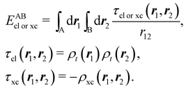 | (61) |
In this expression, a classical nuclear density,
, where α runs over the nuclei and
Z denotes the nuclear charge, has been added to the electron density
ρ to define a total (electronic plus nuclear) charge density,
ρt(
r) =
ρn(
r) −
ρ(
r). We now recall that the covalent bond order, as measured by the delocalization index
δAB, given by
eqn (39) which, apart from the
r12 interelectron distance, is just a scaled
EABxc. Using a bipolar expansion, which is always convergent unlike the more commonly found multipolar expansion,
226 it has been shown
71 that both the covalent and ionic terms can be written as Taylor series in which the leading terms are
| |  | (62) |
| |  | (63) |
where
QA, and
QB are the total (nuclear plus electronic) charges of A and B. In this sense,
ιAB = −
QAQB can be taken as an ionic bond order. Doing so, a total bond order
εAB =
ιAB +
δAB can be defined such that the total interaction energy
EABint ≈ −
εAB/
RAB.
An algebraic relationship is thus uncovered between electron counting descriptors (bond orders) and (in situ) bond energies. Surprisingly, the leading term in the covalent energy contribution follows an inverse power law much as the ionic one. It is very satisfying that a clear model of this behavior is straightforward from the analysis of EDFs. In a purely covalent bond, as examined, the total probability of finding two electrons in one center is 1/4 + 1/4 = 1/2. In these situations a −1/RAB attraction exists between them, leading to an overall −1/(2RAB) interaction. No interaction, to first order, occurs when one electron lies in each neutral center. We believe that this model shows neatly that the origin of all interactions in a Coulombic Hamiltonian is electrostatic in nature.
The first order approximation reproduces reasonably well the exactly computed IQA/QTAIM covalent, ionic, and total interaction energies. Fig. 11 shows this comparison. In most cases, the leading order term of the expansion leads to semi-quantitative agreement with the exactly computed values. We have also shown that the agreement improves considerably if further order in the series expansion of both the covalent and ionic energies is taken into account.227
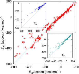 |
| | Fig. 11 Comparison of the leading order covalent (Exc), ionic (Ecl), and total interaction energies (Eint) with their exactly computed values for a set of over 800 different compounds covering several types of bonding regimes. Taken from ref. 228, where more details can be found, with permission granted by the retained rights of the authors. Data are provided in kcal mol−1. | |
7 Recovering one-electron pictures
Regardless of the intrinsic power that real space methods have shown in chemical bonding issues, it cannot be denied that most chemists still use and pursue orbital pictures to rationalize their findings. Since delocalized canonical orbitals do not conform to the standard Lewis image, localized functions have become important in one-particle images of the chemical bond. Being Slater determinants invariant under unitary transformations of their orbitals, many different localization techniques have been devised over the years, like the now standard Edmiston–Ruedenberg229 or Pipek–Mezey230 procedures. Simultaneously, a quest for a simplified description of a complex wavefunction in terms of a set of atomic-like orbitals as close as possible to a minimal basis set has led to well-known procedures, like Weinhold and coworkers' natural bond orbital (NBO) formalism,231 that has been severely criticized (see for instance ref. 232). Newer ideas have not ceased to be proposed, like in the case of the so-called intrinsic atomic orbitals proposed by Knizia,233 or in the adaptive natural density partitioning (AdNDP) method of Zubarev and Boldyrev,234 that allows to tell easily two- from multi-center bonds, and that has been also generalized to solids.235 Clearly, chemists are used to manipulate orbitals in very many clever ways, and it is relevant to examine the possibility of recovering effective one-particle functions from real space methods.
The combined use of a real space partition into fuzzy or non-fuzzy atoms together with an Open Quantum Systems (OQS) perspective of QCT236–238 is a relatively straightforward, yet powerful way to access one-electron images of different flavors. These one-electron functions can be visualized and compared between different systems, as well as with orbitals obtained by other methods as those described in the previous paragraph. Their analyses allow drawing significant conclusions, which are difficult or impossible to obtain in other ways. Among the different existing possibilities, in this work we will only comment on three of them: the domain averaged Fermi hole (DAFH) orbitals, the natural adaptive molecular orbitals (NAdOs), and the fragment natural orbitals (FNO). Interestingly, all of them converge onto the domain natural orbitals (DNO) developed by Ponec in the case of one region and SDWs. When describing how these one-electron functions are obtained, we will only present an illustrative example, without further discussion (see Fig. 12–14), for which we refer the reader to the original references.
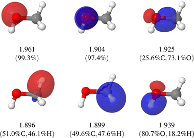 |
| | Fig. 12 |ϕ| = 0.08 a.u. isosurface of the non-core valence 1c and 2c DAFH functions found in methanol at the CCSD(T)//cc-pVDZ level. 1c and 2c occupations and percentage of population localized are also shown. Reproduced from ref. 255 with permission from the Royal Society of Chemistry. | |
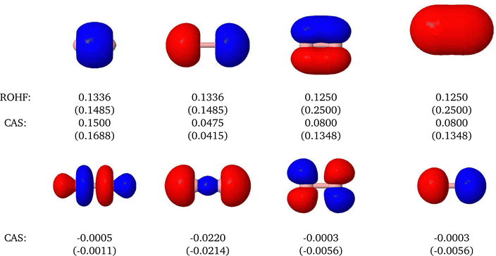 |
| | Fig. 13 |ψ| = 0.05 a.u. isosurfaces for the non-core NAdOs in the B2 and C2 molecules. The numbers below correspond to their respective occupations nabi at the ROHF and CAS levels, with a 6-311G(d,p)++ basis set. C2 data in parenthesis. Reproduced from ref. 256. Copyright 2015 John Wiley and Sons, Inc. | |
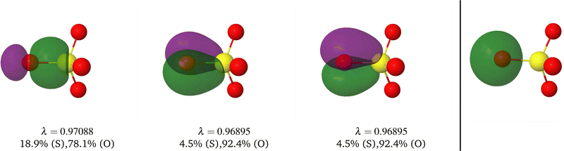 |
| | Fig. 14 |φ| = 0.05 a.u. isosurface of the σ (left) and π (center and right) S–O FNOs of the SO42− anion at the B3LYP//def2-QZVPPD level of calculation. The rightmost graph corresponds to the lone pair of oxygen atom. Reprinted with permission of the authors from ref. 257. | |
7.1 Domain-averaged Fermi hole orbitals (DAFH)
The DAFH molecular orbitals of atom or fragment A are obtained by diagonalizing the exchange–correlation density ρxc2 after one of the electron coordinates has already been integrated over A. In a basis of canonical orbitals ϕi, assuming for simplicity a closed-shell (N = 2n) molecule, real spin–orbitals, and after integrating out the spin variables, we arrive at| |  | (64) |
Threrein, M is the size of the MO basis, and ηijkl are coefficients coming from the expansion of the wavefunction in terms of Slater determinants, with ηijkl = 2δikδjl for SDWs. If electron 2 is integrated over fragment A, the spinless DAFH GA(r) function is obtained:| |  | (65) |
where  . The diagonalization of GA/2 = GAα = GAβ leads to a set of M DAFH MOs ϕAi(r) and their corresponding occupation numbers nAi. The DAFH MOs of highest occupancy for the methanol molecule and their occupation numbers at the CCSD(T)//cc-pVDZ level are provided in Fig. 12. These are well-defined functions obtained at any level of theory that preserve conventional chemical wisdom and that are invariant under orbital tranformations of the underlying wavefunction. Notice how close to two the propulations are, much as in NBO analyses, without the need of the involved and some times ad hoc transformations that lead to natural bond orbitals.
We can use the DAFH to write
| |  | (66) |
where the factor 2 accounts for both the α and β components of
GA, which turn out to be equal in a closed-shell molecule. The above expression was originally derived by Ponec,
239,240 and the analysis of the
ϕAi and
nAi functions was carried out later by Ponec and other authors.
241–250 The formalism has been applied to a very large number of systems, both for fuzzy- and non-fuzzy partitions of space, and at equilibrium and non-equilibrium geometries. DAFHs are also intimately related to the effective atomic orbitals of Mayer,
251 which have been very successfully used by Salvador and coworkers to obtain oxidation states in agreement with the IUPAC's recommendations.
252,253 From now on, we will call the
ϕAi s obtained for SDWs domain natural orbitals (DNOs). In the SDW case,
GA acquires a very simple form, since it is given by
GA = 2
SA, where
SA is the AOM defined in
eqn (26).
The occupation numbers nAi satisfy  , the average number of electrons in A. Given that
  , we also have
 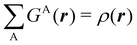 . From eqn (39), (65) and (66), the delocalization index between A and B, δAB, is given by248
| | 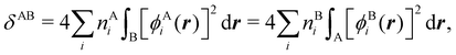 | (67) |
| | 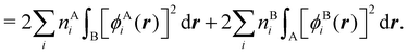 | (68) |
eqn (68) arises due to the symmetry

.
δAB takes a simpler form when the sum of fragments A and B exhaust the system (A∪B =
R3). Then, the first integral in
eqn (68) is equal to 1 −
sAi, where

, and the second becomes 1 −
sBi, where
so
δAB can be written as
| | 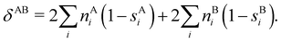 | (69) |
As already stated, both contributions to
δAB are equal. However,
ϕAi ≠
ϕBi and
nAi(1 −
sAi) ≠
nBi(1 −
sBi) in general wavefunctions. Nonetheless, further simplifications in the formalism, very illuminating as regards the relevance of DNOs in chemical bonding theory, take place for SDWs when A∪B =
R3.
254 In this case, using the property
SB =
I −
SA, it can be shown that
ϕAi =
ϕBi, and not only that: DNOs, in addition to being orthonormal in
R3, are also orthogonal in A and B, with 〈
ϕAi|
ϕjA〉
A =
δijsAi =
δij(1 − 〈
ϕBi|
ϕBj〉
B) =
δij(1 −
sBi). Moreover, the occupations of both fragments are related by
nAi = 1 −
nBi, and are equal to the respective overlaps in the fragments,
nAi =
sAi and
nBi =
sBi. In the end, all these transformations allow us to write
eqn (69) as
| | 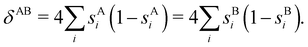 | (70) |
The relevance of the above equation is that it connects the bond order between A and B, measured through δAB, with the localized or delocalized character of the DNOs. A DNO highly localized in A (sAi = 1 − sBi ≃ 1) or in B (sBi = 1 − sAi ≃ 1) hardly contributes to δAB and only those orbitals significantly delocalized in both fragments give rise to significant contributions to the bond order. In an indirect way, the exchange–correlation interaction energy between two fragments A and B (VABxc), as long as A∪B = R3 and the wavefunction is a SDW expressed in terms of the DNOs, is completely dominated by those DNOs with appreciable delocalization in A and B simultaneously. The contribution of those DNOs that are strongly localized in one of the two fragments is very small. This picture offers an extraordinarily coherent image of our electron counting formalism plus IQA energy partitioning method. Expressed in a language quite familiar to chemists: the core electrons of a system (represented in this case by highly localized DNOs in one of the fragments) have little relevance, both from the point of view of the bond order (i.e. the δAB value), as well as from the energetic viewpoint (i.e. the VABxc value).
7.2 Natural adaptive molecular orbitals (NAdOs)
The use of cumulant densities allow for a rather simple generalization of DNOs to the multicenter case. As we have seen, if one electron coordinate of the nth-order cumulant density (nCD), ρcn, is integrated out we recover the (n − 1)th CD (eqn (13)). Taking, for instance, n = 3,| |  | (71) |
Alternatively, if we integrate r1 in a region ΩA and r2 in another region ΩB, what it is obtained is the one-electron function ρab(r)| |  | (72) |
Expressed in the basis {ϕi} of canonical orbitals,| | | ρab(r) = (ϕ1ϕ2⋯)Dab(ϕ1ϕ2⋯)†, | (73) |
where Dab is a symmetric matrix that can be diagonalized. In terms of its eigenvalues {nabi} and eigenvectors {ψabi}| | 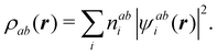 | (74) |
Since 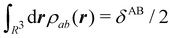 , and each ψabi(r) is normalized, the nabis obey the sum rule
 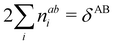 . Thus, 2 × nabi is the contribution of ψabi(r) to the bond order between A and B, and each ψabi itself defines a two-center natural adaptive orbital (NAdO). This means that two-center NAdOs induce a one-electron decomposition of any two-center delocalization index.
The generalization to an arbitrary n is straightforward:256
| |  | (75) |
| | | = (ϕ1ϕ2⋯)Dab⋯n(ϕ1ϕ2⋯)†, | (76) |
and
| |  | (77) |
where {
ψab⋯ni} and {
nab⋯ni} are the
n-center NAdOs and their eigenvalues, respectively. Since
and the
ψab⋯ni(
r)'s are again normalized, the sum rule is now
than can be taken as an
n-center delocalization index. When
n = 1, the generalized density
ρa(
r) coincides with the DAFH function
GA(
r) defined in the previous subsection, and the 1-center NAdOs
ψai(
r) and their eigenvalues
nai's are equal to twice the DAFH occupancies (2
nAi) and DAFH MOs
ϕAi(
r).
The n-center NAdOs provide clear images of n-center bonds, and are adaptively localized or delocalized over the n centers used to compute them. If one NAdO is fully localized over one center, it represents a core or lone-pair orbital of that center and does not contribute to any n-center bond (n > 1). If one of the NAdOs is completely localized over n centers, it describes a pure n-center bond. In contrast, a NAdO which is only partly localized on n centers signals the existence of higher order multicenter bonding. For instance, NAdOs obtained for n = 1 can be fully localized on one center (i.e. they describe core or lone pair orbitals) or delocalized over two or more centers, describing in this second case the existence of at least two-center bonding. This means that the NAdOS obtained by diagonalizing ρa(r) can be used to analyze chemical bonds in real space if we focus our attention on their delocalized components. This procedure is, in fact, the usual way in which Ponec's DAFHs have generally been used since they were proposed. Nonetheless, we note that the formalism just introduced is more suitable for this purpose. Moreover, n-center NAdOs obtained as described here transform according to the irreducible representations of the group of the n centers involved in obtaining them. No a posteriori matrix transformation as, for instance, an isopycnic rotation, is necessary to achieve this.
As an example, the valence NAdOs obtained for the B2 and C2 molecules, described at the restricted open shell HF (ROHF) as well as the CAS levels are shown in Fig. 13. It can be clearly seen that their shape is easily interpreted with standard chemical wisdom, and that we clearly isolate σ or π contributions as in standard molecular orbital theory. NAdOs, however, contain extra information, since their occupation numbers measure their contribution to the total bond order. Thus we see that both in dicarbon and diboron the σg and σu functions contribute considerably to bonding at the mean-field level, leading to a close to quadruple bond image in C2, but that the σu function becomes considerably less important upon inclusion of correlation.
7.3 Fragment natural orbitals (FNOs)
Much as in the NBO paradigm it is the atomic blocks of the 1RDM written in an atom-centered basis which is diagonalized to provide natural atomic orbitals,231 the consideration of an atom or fragment in real space as an open quantum system (OQS) can be used to define real space analogues of an atomic RDMs. We call fragment natural orbitals (FNOs) the orbitals obtained for a fragment A of a molecule after diagonalizing its OQS 1RDM. It can be shown238 that the 1RDM of an atom or fragment A can be written as ρA(r;r′) = ωA(r)ωA(r′)ρ(r;r′), where ωA is a weight factor as defined above (when A is a single atom) or the sum of the weight factors of all the atoms that make up the fragment otherwise, and ρ(r;r′) is the standard 1RDM of the whole molecule. When the latter is expressed in a basis of orthonormal orbitals |ui〉,| |  | (78) |
ρA(r;r′) results| | | ρA(r;r′) = ωA(r)|u〉ρ〈u|ωA(r′). | (79) |
The matrix representation of ρA(r;r′) in the |ui〉 basis is simply SAρSA, where SA is the standard AOM matrix (eqn (26)) when A is an atom, or the sum of the AOMs of all the atoms that make up the fragment A. The FNOs of this fragment are obtained by diagonalizing SAρSA, taking care that the basis |ui〉 is not orthonormal in A. This is equivalent to diagonalize ρA = (SA)1/2ρ(SA)1/2, i.e. ρAU = Udiag(λA). An alternative possibility is to first express the standard 1RDM in the Löwdin orthogonalized basis |up〉, defined as |up〉 = |u〉(SA)−1/2. In this basis, the matrix representation of ρA(r;r′) is directly ρA. Be that as it may, FNOs of fragment A are given by |φ〉 = |up〉U = |u〉 (SA)−1/2U ≡ |u〉C. The φi functions are orthonormal in A but not in R3, since 〈φ|φ〉R3 = U†(SA)−1U = C†C ≠ I.
In SDWs, ρ = 2I (where I is the identity matrix) and, therefore, ρA = (SA)1/2ρ(SA)1/2 = 2SA, so that the matrix representation of ρA(r;r′) coincides with twice the AOM in fragment A. In other words, ρA it is equal to the GA matrix that is diagonalized in the derivation of Ponec's DNOs. This means that DNOs and FNOs are the same in this case, as well as their respective occupations, λAi = 2nAi. Furthermore, since SA is positive definite, all λAis are greater than zero, so there are no DNOs or FNOs with negative occupations in case of SDWs. This equivalence between DNOs and FNOs in SDWs extends also to 1- and 2-center NAdOs provided that A∪B = R3, since Da = SA, Db = SB, and Dab = (SASB + SBSA)/2 in SDWs. The diagonalization of these three matrices lead to the same eigenvectors, ψai = ψbi = ψabi, for SB = I − SA. Moreover, occupations derived from Da and Db are related by nai = 1 − nbi and each nai is the self-overlap integral of ψai in A, 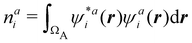 .
.
We took the SO42− anion as an example to illustrate FNOs. In Fig. 14 we present the bonding FNOs for one of the four equivalent S–O pairs, as well as the oxygen lone pair FNO. As we clearly see, there is a triple S–O bond (one σ and two equivalent π bonds).
8 Summary and conclusions
We have reviewed in this perspective some recent advances in the concept of an atom-in-a-molecule from a real space viewpoint. We have shown that both fuzzy and non-fuzzy decompositions can be dealt with, on the same footing, when atomic weight functions are used and have examined a few of the best-known weights in both categories. Once an atom (or fragment) is so defined, a wealth of chemically relevant information becomes accessible by using reduced densities or density matrices and their irreducible parts, the so-called cumulant densities or density matrices. We have stressed how the expectation value of any operator can be written as a sum of atomic contributions. This is not the case in many other methodologies. When the expectation values of the densities themselves are partitioned, we obtain atomic, interatomic, or, in general, polyatomic populations that provide, in the limit, the full statistical electron distribution function. The relationship between the fluctuation of the atomic or fragment populations and the real space multicenter bond orders has been highlighted. This link is particularly important, and not so well known. When the total Hamiltonian operator is partitioned instead, an energy decomposition arises, the interacting quantum atoms (IQA) method, which writes the total energy of a system as a sum of atomic or fragment self-energies and pairwise additive interatomic (interfragment) interactions. We have focused on recent expansions of IQA to intermolecular interactions and biologically important compounds. A straightforward link between electron counting and IQA has also been reviewed. Finally, a means to recover one-electron functions, i.e. orbitals, from real space partitions, has also been provided.
The definition of an atom-in-a-molecule as a real space object provides a unique way to examine the spatial distribution of the electrons in a molecule. By adopting this viewpoint, fully compatible with the underlying quantum mechanical reality, the chemist's language shifts from orbitals (which if endowed with an energetic signature must be delocalized) to interactions. Instead of isolating electrons from nuclei and considering more or less delocalized objects that exactly host one or two electrons, the real space perspective considers spatial regions associated with interacting atoms or fragments. These regions do not possess an immutable but a fluctuating number of particles. The fluctuations can be followed if the probabilities of finding a given partition of the electrons in the set of atomic regions, i.e. the electron distribution function, are computed. The number of atoms involved in these population fluctuations decides whether we have two-center or multi-center bonds, which can be visualized by building appropriate one-electron functions that further decompose bond orders using an orbital-like narrative.
Author contributions
Conceptualization: AMP and EFM. Funding acquisition: AMP and TRR. Investigation: AMP, EFM, DS, AC, ND, JM, TRR, and JMG. Writing-original draft: AMP, EFM, DS, AC, ND, JM, TRR, and JMG. Project administration: AMP.
Conflicts of interest
There are no conflicts to declare.
Acknowledgements
We acknowledge the spanish MICINN, grant PID2021-122763NB-I00 and the FICyT, grant IDI/2021/000054 for financial support. TRR gratefully acknowledges DGTIC/UNAM for computer time (LANCAD-UNAM-DGTIC 250).
References
- C. A. Coulson, Rev. Mod. Phys., 1960, 32, 170–177 CrossRef CAS.
- F. Neese, M. Atanasov, G. Bistoni, D. Maganas and S. Ye, J. Am. Chem. Soc., 2019, 141, 2814–2824 CrossRef CAS PubMed.
- K. T. Butler, D. W. Davies, H. Cartwright, O. Isayev and A. Walsh, Nature, 2018, 559, 547–555 CrossRef CAS PubMed.
- A. Aspuru-Guzik, M.-H. Baik, S. Balasubramanian, R. Banerjee, S. Bart, N. Borduas-Dedekind, S. Chang, P. Chen, C. Corminboeuf, F.-X. Coudert, L. Cronin, C. Crudden, T. Cuk, A. G. Doyle, C. Fan, X. Feng, D. Freedman, S. Furukawa, S. Ghosh, F. Glorius, M. Jeffries-EL, N. Katsonis, A. Li, S. S. Linse, S. Marchesan, N. Maulide, A. Milo, A. R. H. Narayan, P. Naumov, C. Nevado, T. Nyokong, R. Palacin, M. Reid, C. Robinson, G. Robinson, R. Sarpong, C. Schindler, G. S. Schlau-Cohen, T. W. Schmidt, R. Sessoli, Y. Shao-Horn, H. Sleiman, J. Sutherland, A. Taylor, A. Tezcan, M. Tortosa, A. Walsh, A. J. B. Watson, B. M. Weckhuysen, E. Weiss, D. Wilson, V. W.-W. Yam, X. Yang, J. Y. Ying, T. Yoon, S.-L. You, A. J. G. Zarbin and H. Zhang, Nat. Chem., 2019, 11, 286–294 CrossRef CAS PubMed.
- J. M. Galbraith, S. Shaik, D. Danovich, B. Braïda, W. Wu, P. Hiberty, D. L. Cooper, P. B. Karadakov and T. H. Dunning, J. Chem. Educ., 2021, 98, 3617–3620 CrossRef CAS.
- M. Kohout, K. Pernal, F. R. Wagner and Y. Grin, Theor. Chem. Acc., 2004, 112, 453–459 Search PubMed.
- M. Kohout, K. Pernal, F. R. Wagner and Y. Grin, Theor. Chem. Acc., 2005, 113, 287–293 Search PubMed.
- M. Kohout, F. R. Wagner and Y. Grin, Theor. Chem. Acc., 2007, 119, 413–420 Search PubMed.
- K. Ruedenberg and M. W. Schmidt, J. Phys. Chem. A, 2009, 113, 1954–1968 CrossRef CAS PubMed.
- W. A. Kato, Commun. Pure Appl. Math., 1957, 10, 151 CrossRef.
- P. Hohenberg and W. Kohn, Phys. Rev., 1964, 136, B864–B871 CrossRef.
-
R. F. W. Bader, Atoms in Molecules, Oxford University Press, Oxford, 1990 Search PubMed.
- J. M. Guevara-Vela, E. Francisco, T. Rocha-Rinza and Á. Martín Pendás, Molecules, 2020, 25, 4028 CrossRef CAS PubMed.
- E. Francisco, Á. Martín Pendás and M. A. Blanco, J. Chem. Theory Comput., 2006, 2, 90–102 CrossRef CAS PubMed.
-
Á. Martín Pendás, M. Kohout, M. A. Blanco and E. Francisco, in Modern Charge-density analysis, ed. C. Gatti and P. Macchi, Springer, Dordrecht., 2012, p. 165 Search PubMed.
-
C. Kittel, Introduction to solid state physics, John Wiley & Sons, Nashville, TN, 8th edn, 2004 Search PubMed.
- J. C. Slater, J. Chem. Phys., 1964, 41, 3199–3204 CrossRef CAS.
- R. F. W. Bader, T. T. Nguyen-Dang and Y. Tal, Rep. Prog. Phys., 1981, 44, 893–948 CrossRef.
- J. S. M. Anderson, P. W. Ayers and J. I. R. Hernandez, J. Phys. Chem. A, 2010, 114, 8884–8895 CrossRef CAS PubMed.
- A. D. Becke and K. E. Edgecombe, J. Chem. Phys., 1990, 92, 5397–5403 CrossRef CAS.
- B. Silvi and A. Savin, Nature, 1994, 371, 683–686 CrossRef CAS.
- V. Polo, J. Andres, S. Berski, L. R. Domingo and B. Silvi, J. Phys. Chem. A, 2008, 112, 7128–7136 CrossRef CAS PubMed.
- J. Andrés, S. Berski and B. Silvi, Chem. Commun., 2016, 52, 8183–8195 RSC.
- M. Kohout, Int. J. Quantum Chem., 2003, 97, 651–658 CrossRef.
- In Chemical applications of atomic and molecular electrostatic potentials, ed. P. Politzer and D. G. Truhlar, Springer, New York, NY, 1981st edn, 1981 Search PubMed.
- S. R. Gadre and R. D. Bendale, Chem. Phys. Lett., 1986, 130, 515–521 CrossRef CAS.
- S. R. Gadre, S. A. Kulkarni and I. H. Shrivastava, J. Chem. Phys., 1992, 96, 5253–5260 CrossRef CAS.
- I. Mata, E. Molins and E. Espinosa, J. Phys. Chem. A, 2007, 111, 9859–9870 CrossRef CAS PubMed.
- S. R. Gadre, C. H. Suresh and N. Mohan, Molecules, 2021, 26, 3289 CrossRef CAS PubMed.
- Á. Martín Pendás and J. Hernández-Trujillo, J. Chem. Phys., 2012, 137, 134101 CrossRef PubMed.
- J. Dillen, J. Comput. Chem., 2015, 36, 883–890 CrossRef CAS PubMed.
- V. Tsirelson and A. Stash, Acta Crystallogr., Sect. B: Struct. Sci., Cryst. Eng. Mater., 2020, 76, 769–778 CrossRef CAS PubMed.
- N. O. J. Malcolm and P. L. A. Popelier, Faraday Discuss., 2003, 124, 353 RSC.
- P. Popelier, Coord. Chem. Rev., 2000, 197, 169–189 CrossRef CAS.
- B. Landeros-Rivera, M. Gallegos, J. Munárriz, R. Laplaza and J. Contreras-García, Phys. Chem. Chem. Phys., 2022, 24, 21538–21548 RSC.
- Á. Martín Pendás, M. A. Blanco, A. Costales, P. M. Sánchez and V. Luaña, Phys. Rev. Lett., 1999, 83, 1930–1933 CrossRef.
- R. Saha, P. Das and P. K. Chattaraj, ChemPhysChem, 2022, e202200329-1-17 Search PubMed.
- M. Marqués, M. I. McMahon, E. Gregoryanz, M. Hanfland, C. L. Guillaune, C. J. Pickard, G. J. Ackland and R. J. Nelmes, Phys. Rev. Lett., 2011, 106, 095502 CrossRef PubMed.
- V. Postils, M. Garcia-Borràs, M. Solà, J. M. Luis and E. Matito, Chem. Commun., 2015, 51, 4865–4868 RSC.
- S. Noorizadeh, Chem. Phys. Lett., 2016, 652, 40–45 CrossRef CAS.
- Á. Martín Pendás, E. Francisco, M. Blanco and C. Gatti, Chem. – Eur. J., 2007, 13, 9362–9371 CrossRef PubMed.
- S. Shahbazian, Chem. – Eur. J., 2018, 24, 5401–5405 CrossRef CAS PubMed.
- M. Yu and D. R. Trinkle, J. Chem. Phys., 2011, 134, 064111 CrossRef PubMed.
- M. Goli and S. Shahbazian, Theor. Chem. Acc., 2013, 132, 1365 Search PubMed.
- M. Goli and S. Shahbazian, Phys. Chem. Chem. Phys., 2014, 16, 6602 RSC.
- M. Goli and S. Shahbazian, ChemPhysChem, 2019, 20, 831–837 CrossRef CAS PubMed.
-
S. Shahbazian, Advances in Quantum Chemical Topology Beyond QTAIM, Elsevier, 2023, pp. 73–109 Search PubMed.
- A. D. Becke, J. Chem. Phys., 1988, 88, 2547–2553 CrossRef CAS.
- P. Salvador and E. Ramos-Cordoba, J. Chem. Phys., 2013, 139, 071103 CrossRef PubMed.
- C. Fonseca Guerra, J.-W. Handgraaf, E. J. Baerends and F. M. Bickelhaupt, J. Comput. Chem., 2003, 25, 189–210 CrossRef PubMed.
- A. N. Petelski and C. Fonseca Guerra, Chem. – Asian J., 2022, 17, e202201010 CAS.
- D. Svatunek, T. Hansen, K. N. Houk and T. A. Hamlin, J. Org. Chem., 2021, 86, 4320–4325 CrossRef CAS PubMed.
- A. M. Köster, R. Flores-Moreno and J. U. Reveles, J. Chem. Phys., 2004, 121, 681–690 CrossRef PubMed.
- R. Stratmann, G. E. Scuseria and M. J. Frisch, Chem. Phys. Lett., 1996, 257, 213–223 CrossRef CAS.
- F. L. Hirshfeld, Theor. Chem. Acc., 1977, 44, 129–138 Search PubMed.
- K. Kullback and R. A. Leibler, Ann. Math. Statistics, 1951, 22, 79 Search PubMed.
-
R. F. Nalewajski, Information origins of the chemical bond, Nova Science, Hauppauge, NY, 2010 Search PubMed.
- P. Bultinck, C. V. Alsenoy, P. W. Ayers and R. Carbó-Dorca, J. Chem. Phys., 2007, 126, 144111 CrossRef PubMed.
- K. Finzel, Á. Martín Pendás and E. Francisco, J. Chem. Phys., 2015, 143, 084115 CrossRef PubMed.
- F. Heidar-Zadeh, P. W. Ayers, T. Verstraelen, I. Vinogradov, E. Vöhringer-Martinez and P. Bultinck, J. Phys. Chem. A, 2017, 122, 4219–4245 CrossRef PubMed.
- T. C. Lillestolen and R. J. Wheatley, J. Chem. Phys., 2009, 131, 144101 CrossRef PubMed.
- J. F. Rico, R. López and G. Ramírez, J. Chem. Phys., 1999, 110, 4213–4220 CrossRef CAS.
- R. McWeeny, Rev. Mod. Phys., 1960, 32, 335–369 CrossRef.
- E. Francisco, Á. Martín Pendás and M. A. Blanco, J. Chem. Phys., 2007, 126, 094102-1–094102-13 Search PubMed.
- C. Outeiral, M. A. Vincent, A. Martín Pendás and P. L. A. Popelier, Chem. Sci., 2018, 9, 5517–5529 RSC.
- I. Mayer, Chem. Phys. Lett., 1983, 97, 270–274 CrossRef CAS.
- M. S. Giambiagi, M. Giambiagi and F. E. Jorge, Theor. Chim. Acta, 1985, 68, 337–341 CrossRef.
- J. G. Ángyán, E. Rosta and P. R. Surján, Chem. Phys. Lett., 1999, 299, 1–8 CrossRef.
- A. Julg and P. Julg, Int. J. Quantum Chem., 1978, 13, 483–497 CrossRef CAS.
- M. A. Blanco, Á. Martín Pendás and E. Francisco, J. Chem. Theory Comput., 2005, 1, 1096–1109 CrossRef CAS PubMed.
- E. Francisco, D. Menéndez-Crespo, A. Costales and Á. Martín Pendás, J. Comput. Chem., 2017, 38, 816–829 CrossRef CAS PubMed.
- W. Kutzelnigg and D. Mukherjee, J. Chem. Phys., 1999, 110, 2800–2809 CrossRef CAS.
- P. Ziesche, Int. J. Quantum Chem., 1996, 60, 1361–1374 CrossRef.
- C. Aslangul, R. Constanciel and R. Daudel, Adv.
Quantum Chem., 1972, 6, 93–141 CrossRef CAS.
- E. Francisco, Á. Martín Pendás and M. A. Blanco, Comput. Phys. Commun., 2008, 178, 621–634 CrossRef CAS.
- E. Francisco, Á. Martín Pendás, M. García-Revilla and R. Álvarez Boto, Comput. Theor. Chem., 2013, 1003, 71–78 CrossRef CAS.
- M. Giambiagi, M. S. de Giambiagi and K. C. Mundim, Struct. Chem., 1990, 1, 423–427 CrossRef CAS.
- K. C. Mundim, M. Giambiagi and M. S. de Giambiagi, J. Phys. Chem., 1994, 98, 6118–6119 CrossRef CAS.
- R. Ponec, P. Bultinck and A. G. Saliner, J. Phys. Chem. A, 2005, 109, 6606–6609 CrossRef CAS PubMed.
- R. Bochicchio, R. Ponec, A. Torre and L. Lain, Theor. Chem. Acc., 2001, 105, 292–298 Search PubMed.
- L. Lain, A. Torre, R. Bochicchio and R. Ponec, Chem. Phys. Lett., 2001, 346, 283–287 CrossRef CAS.
- A. Torre, L. Lain and R. Bochicchio, J. Phys. Chem. A, 2002, 107, 127–130 CrossRef.
- R. Bochicchio, L. Lain and A. Torre, J. Comput. Chem., 2003, 24, 1902–1909 CrossRef CAS PubMed.
- R. C. Bochicchio, A. Torre and L. Lain, J. Chem. Phys., 2005, 122, 084117 CrossRef CAS PubMed.
- A. Torre, D. R. Alcoba, L. Lain and R. C. Bochicchio, J. Phys. Chem. A, 2010, 114, 2344–2349 CrossRef CAS PubMed.
- D. R. Alcoba, A. Torre, L. Lain and R. C. Bochicchio, J. Chem. Theory Comput., 2011, 7, 3560–3566 CrossRef CAS PubMed.
- E. Cancès, R. Keriven, F. Lodier and A. Savin, Theor. Chem. Acc., 2004, 111, 373–380 Search PubMed.
- Á. Martín Pendás, E. Francisco and M. A. Blanco, J. Chem. Phys., 2007, 127, 144103-1–144103-9 CrossRef PubMed.
- E. Francisco, Á. Martín Pendás and M. A. Blanco, Theor. Chem. Acc., 2010, 128, 433–444 Search PubMed.
- E. Chamorro, P. Fuentealba and A. Savin, J. Comput. Chem., 2003, 24, 496–504 CrossRef CAS PubMed.
- A. Gallegos, R. Carbó-Dorca, F. Lodier, E. Cancès and A. Savin, J. Comput. Chem., 2005, 26, 455–460 CrossRef CAS PubMed.
-
O. M. Lopes, B. Braïda, M. Causà and A. Savin, Advances in the Theory of Quantum Systems in Chemistry and Physics, Springer, Netherlands, 2011, pp. 173–184 Search PubMed.
- M. Menéndez and A. M. Pendás, Theor. Chem. Acc., 2014, 133, 1539 Search PubMed.
- M. Causà and A. Savin, J. Phys. Chem. A, 2011, 115, 13139–13148 CrossRef PubMed.
- A. Scemama, M. Caffarel and A. Savin, J. Comput. Chem., 2006, 28, 442–454 CrossRef PubMed.
- G. Acke, S. D. Baerdemacker, P. W. Claeys, M. V. Raemdonck, W. Poelmans, D. V. Neck and P. Bultinck, Mol. Phys., 2016, 114, 1392–1405 CrossRef CAS.
- D. V. Hende, L. Lemmens, S. D. Baerdemacker, D. V. Neck, P. Bultinck and G. Acke, J. Comput. Chem., 2022, 43, 457–464 CrossRef PubMed.
- Á. Martín Pendás and E. Francisco, ChemPhysChem, 2019, 20, 2722–2741 CrossRef PubMed.
- R. F. W. Bader and M. E. Stephens, J. Am. Chem. Soc., 1975, 97, 7391 CrossRef CAS.
- R. F. W. Bader and M. E. Stephens, Chem. Phys. Lett., 1974, 26, 445–449 CrossRef CAS.
-
Y. Grin, A. Savin and B. Silvi, The Chemical Bond, Wiley-VCH Verlag GmbH & Co. KGaA, 2014, pp. 345–382 Search PubMed.
- B. Silvi and E. Alikhani, J. Chem. Phys., 2022, 156, 244305 CrossRef CAS PubMed.
- K. Wiberg, Tetrahedron, 1968, 24, 1083–1096 CrossRef CAS.
- I. Mayer, J. Comput. Chem., 2006, 28, 204–221 CrossRef PubMed.
- J. L. Casals-Sainz, J. Jara-Cortés, J. Hernández-Trujillo, J. M. Guevara-Vela, E. Francisco and Á. Martín Pendás, Chem. – Eur. J., 2019, 25, 12169–12179 CrossRef CAS PubMed.
- Á. Martn Pendás, E. Francisco and M. A. Blanco, Phys. Chem. Chem. Phys., 2007, 9, 1087–1092 RSC.
- J. L. Casals-Sainz, F. Jiménez-Grávalos, E. Francisco and Á. Martín Pendás, Chem. Commun., 2019, 55, 5071–5074 RSC.
- L. Zhao, M. Hermann, W. H. E. Schwarz and G. Frenking, Nat. Rev. Chem., 2019, 3, 48–63 CrossRef CAS.
- B. Jeziorski, R. Moszynski and K. Szalewicz, Chem. Rev., 1994, 94, 1887–1930 CrossRef CAS.
- K. Kitaura and K. Morokuma, Int. J. Quantum Chem., 1976, 10, 325–340 CrossRef CAS.
- K. Morokuma, Acc. Chem. Res., 1977, 10, 294–300 CrossRef CAS.
- T. Ziegler and A. Rauk, Inorg. Chem., 1979, 18, 1558–1565 CrossRef CAS.
- L. Zhao, M. von Hopffgarten, D. M. Andrada and G. Frenking, Wiley Interdiscip. Rev.: Comput. Mol. Sci., 2017, 8, e1345-1-37 Search PubMed.
-
F. M. Bickelhaupt and E. J. Baerends, Rev. Comp. Chem., John Wiley & Sons, Inc., 2007, pp. 1–86 Search PubMed.
- D. S. Levine and M. Head-Gordon, Proc. Natl. Acad. Sci. U. S. A., 2017, 114, 12649–12656 CrossRef CAS PubMed.
- Á. Martín Pendás, M. A. Blanco and E. Francisco, J. Comput. Chem., 2007, 28, 161–184 CrossRef PubMed.
- Á. Martín Pendás, M. A. Blanco and E. Francisco, J. Chem. Phys., 2006, 125, 184112-1–184112-20 CrossRef PubMed.
- D. Tiana, E. Francisco, M. A. Blanco, P. Macchi, A. Sironi and Á. Martín Pendás, J. Chem. Theory Comput., 2010, 6, 1064–1074 CrossRef CAS.
- Á. Martín Pendás, M. A. Blanco and E. Francisco, J. Comput. Chem., 2009, 30, 98–109 CrossRef PubMed.
- Á. Martín Pendás and E. Francisco, Nat. Commun., 2022, 13, 3327-1-10 Search PubMed.
-
E. Francisco and A. Martín Pendás, in Non-covalent Interactions in Quantum Chemistry and Physics, ed. A. Otero-de-la Roza and G. DiLabio, Elsevier, Amsterdam, 2017, ch. Energy Partition Analyses: Symmetry-Adapted Perturbation Theory and Other Techniques, pp. 27–64 Search PubMed.
- S. Racioppi, A. Sironi and P. Macchi, Phys. Chem. Chem. Phys., 2020, 22, 24291–24298 RSC.
- E. Francisco, J. L. Casals-Sainz, T. Rocha-Rinza and A. Martín Pendás, Theor. Chem. Acc., 2016, 135, 1–8 Search PubMed.
- P. Maxwell, Á. Martín Pendás and P. L. A. Popelier, Phys. Chem. Chem. Phys., 2016, 18, 20986–21000 RSC.
- J. L. Casals-Sainz, J. M. Guevara-Vela, E. Francisco, T. Rocha-Rinza and Á. Martín Pendás, J. Comput. Chem., 2020, 41, 1234–1241 CrossRef CAS PubMed.
- L. F. Feitosa, R. B. Campos and W. E. Richter, J. Mol. Graphics, 2023, 118, 108326 CrossRef CAS PubMed.
- I. Cukrowski, Wiley Interdiscip. Rev.: Comput. Mol. Sci., 2021, 12, e1579 Search PubMed.
- I. Cukrowski, D. M. E. van Niekerk and J. H. de Lange, Struct. Chem., 2017, 28, 1429–1444 CrossRef CAS.
- J. H. de Lange, D. M. E. van Niekerk and I. Cukrowski, Phys. Chem. Chem. Phys., 2019, 21, 20988–20998 RSC.
- I. Cukrowski and P. Mangondo, J. Comput. Chem., 2016, 37, 1373–1387 CrossRef CAS PubMed.
- Á. Martín-Pendas, E. Francisco and M. A. Blanco, Chem. Phys. Lett., 2008, 454, 396–403 CrossRef.
- J. Munárriz, R. Laplaza, Á. Martín Pendás and J. Contreras-García, Phys. Chem. Chem. Phys., 2019, 21, 4215–4223 RSC.
- J. Munárriz, M. Gallegos, J. Contreras-García and Á. Martín Pendás, Molecules, 2021, 26, 513 CrossRef PubMed.
- J. M. Guevara-Vela, R. Chávez-Calvillo, M. García-Revilla, J. Hernández-Trujillo, O. Christiansen, E. Francisco, Á. MartínPendás and T. Rocha-Rinza, Chem. – Eur. J., 2013, 19, 14304–14315 CrossRef CAS PubMed.
- J. M. Guevara-Vela, E. Romero-Montalvo, A. Costales, Á. Martín Pendás and T. Rocha-Rinza, Phys. Chem. Chem. Phys., 2016, 18, 26383–26390 RSC.
- T. Steiner, Angew. Chem., Int. Ed., 2002, 41, 48–76 CrossRef CAS.
- V. M. Castor-Villegas, J. M. Guevara-Vela, W. E. V. Narváez, Á. Martín Pendás, T. Rocha-Rinza and A. Fernández-Alarcón, J. Comput. Chem., 2020, 41, 2266–2277 CrossRef CAS PubMed.
- C. Foroutan-Nejad, Z. Badri and R. Marek, Phys. Chem. Chem. Phys., 2015, 17, 30670–30679 RSC.
- M. A. Niyas, R. Ramakrishnan, V. Vijay, E. Sebastian and M. Hariharan, J. Am. Chem. Soc., 2019, 141, 4536–4540 CrossRef CAS PubMed.
- F. Jimeńez-Grávalos, M. Gallegos, Á. Martín-Pendás and A. S. Novikov, J. Comput. Chem., 2021, 42, 676–687 CrossRef PubMed.
- W. E. V. Narváez, E. I. Jiménez, E. Romero-Montalvo, A. S. de la Vega, B. Quiroz-García, M. Hernández-Rodríguez and T. Rocha-Rinza, Chem. Sci., 2018, 9, 4402–4413 RSC.
- W. E. V. Narváez, E. I. Jiménez, M. Cantú-Reyes, A. K. Yatsimirsky, M. Hernández-Rodríguez and T. Rocha-Rinza, Chem. Commun., 2019, 55, 1556–1559 RSC.
- C. F. Matta, J. Hernández-Trujillo, T.-H. Tang and R. F. W. Bader, Chem. – Eur. J., 2003, 9, 1940–1951 CrossRef CAS PubMed.
- J. Poater, M. Solà and F. M. Bickelhaupt, Chem. – Eur. J., 2006, 12, 2889–2895 CrossRef CAS PubMed.
- J. Poater, M. Solà and F. M. Bickelhaupt, Chem. – Eur. J., 2006, 12, 2902–2905 CrossRef CAS PubMed.
- K. Eskandari and C. V. Alsenoy, J. Comput. Chem., 2014, 35, 1883–1889 CrossRef CAS PubMed.
- P. Matczak, Bull. Chem. Soc. Jpn., 2016, 89, 92–102 CrossRef CAS.
- P. L. A. Popelier, P. I. Maxwell, J. C. R. Thacker and I. Alkorta, Theor. Chem. Acc., 2018, 138, 12-1-16 Search PubMed.
- M. P. Mitoraj, F. Sagan, D. W. Szczepanik, J. H. Lange, A. L. Ptaszek, D. M. E. Niekerk and I. Cukrowski, ChemPhysChem, 2020, 21, 494–502 CrossRef CAS PubMed.
-
J. Clayden, N. Greeves and S. Warren, Organic Chemistry, Oxford University Press, London, England, 2nd edn, 2012 Search PubMed.
- A. L. Wilson and P. L. A. Popelier, J. Phys. Chem. A, 2016, 120, 9647–9659 CrossRef CAS PubMed.
- R. A. Buckingham, Proc. R. Soc. London, Ser. A, 1938, 168, 264–283 CAS.
- B. C. B. Symons, D. J. Williamson, C. M. Brooks, A. L. Wilson and P. L. A. Popelier, ChemistryOpen, 2019, 8, 560–570 CrossRef CAS PubMed.
- M. Gallegos, A. Costales and Á. Martín Pendás, ChemPhysChem, 2021, 22, 775–787 CrossRef CAS PubMed.
- J. Jara-Cortes, B. Landeros-Rivera and J. Hernandez-Trujillo, Phys. Chem. Chem. Phys., 2018, 20, 27558–27570 RSC.
- M. Gallegos, A. Costales and Á. Martín Pendás, J. Phys. Chem. A, 2022, 126, 1871–1880 CrossRef CAS PubMed.
- J. L. Casals-Sainz, E. Francisco and Á. Martin Pendas, Z. Anorg. Allg. Chem., 2020, 646, 1062–1072 CrossRef CAS.
- E. Romero-Montalvo, J. M. Guevara-Vela, W. E. V. Narváez, A. Costales, Á. Martín Pendás, M. Hernández-Rodríguez and T. Rocha-Rinza, Chem. Commun., 2017, 53, 3516–3519 RSC.
- A. Sauza-de la Vega, H. Salazar-Lozas, W. E. V. Narváez, M. Hernández-Rodríguez and T. Rocha-Rinza, Org. Biomol. Chem., 2021, 19, 6776–6780 RSC.
- C. Barrales-Martinez, S. Gutierrez-Oliva, A. Toro-Labbe and A. Martin-Pendas, ChemPhysChem, 2021, 22, 1976–1988 CrossRef CAS PubMed.
- J. Jara-Cortes, E. Leal-Sanchez and J. Hernandez-Trujillo, J. Phys. Chem. A, 2020, 124, 6370–6379 CrossRef CAS PubMed.
- J. C. R. Thacker and P. L. A. Popelier, Theor. Chem. Acc., 2017, 136, 86-1-13 Search PubMed.
- A. Fernández-Alarcón, J. M. Guevara-Vela, J. L. Casals-Sainz, A. Costales, E. Francisco, Á. Martín Pendás and T. R. Rinza, Chem. – Eur. J., 2020, 26, 17035–17045 CrossRef PubMed.
- J. Jara-Cortés, J. M. Guevara-Vela, Á. Martín Pendás and J. Hernández-Trujillo, J. Comput. Chem., 2017, 38, 957–970 CrossRef PubMed.
- A. Fernández-Alarcón, J. L. Casals-Sainz, J. M. Guevara-Vela, A. Costales, E. Francisco, Á. Martín Pendás and T. Rocha-Rinza, Phys. Chem. Chem. Phys., 2019, 21, 13428–13439 RSC.
- A. Sauza-de la Vega, L. J. Duarte, A. F. Silva, J. M. Skelton, T. Rocha-Rinza and P. L. A. Popelier, Phys. Chem. Chem. Phys., 2022, 24, 11278–11294 RSC.
- F. Sagan, R. Filas and M. Mitoraj, Crystals, 2016, 6, 28 CrossRef.
- M. A. Niyas, R. Ramakrishnan, V. Vijay and M. Hariharan, Chem. – Eur. J., 2018, 24, 12318–12329 CrossRef CAS PubMed.
- A. T. John, A. Narayanasamy, D. George and M. Hariharan, Cryst. Growth Des., 2022, 22, 1237–1243 CrossRef CAS.
- D. M. Crespo, F. R. Wagner, E. Francisco, Á. Martín Pendás, Y. Grin and M. Kohout, J. Phys. Chem. A, 2021, 125, 9011–9025 CrossRef PubMed.
- K. D. Vogiatzis, M. V. Polynski, J. K. Kirkland, J. Townsend, A. Hashemi, C. Liu and E. A. Pidko, Chem. Rev., 2019, 119, 2453–2523 CrossRef CAS PubMed.
- S. Sowlati-Hashjin, V. Sadek, S. Sadjaji, M. Karttunen, Á. Martín Pendás and C. Foroutan-Nejad, Nat. Commun., 2022, 13, 2069-1-9 Search PubMed.
- C. Werlé, C. Bailly, L. Karmazin-Brelot, X.-F. LeGoff, M. Pfeffer and J.-P. Djukic, Angew. Chem., Int. Ed., 2014, 53, 9827–9831 CrossRef PubMed.
- A. Caballero-Muñoz, J. M. Guevara-Vela, A. Fernández-Alarcón, M. A. Valentín-Rodríguez, M. Flores-Álamo, T. Rocha-Rinza, H. Torrens and G. Moreno-Alcántar, Eur. J. Inorg. Chem., 2021, 2702–2711 CrossRef.
- C. Lacaze-Dufaure, Y. Bulteau, N. Tarrat, D. Loffreda, P. Fau, K. Fajerwerg, M. L. Kahn, F. Rabilloud and C. Lepetit, Inorg. Chem., 2022, 61, 7274–7285 CrossRef CAS PubMed.
- J. M. Guevara-Vela, K. Hess, T. Rocha-Rinza, Á. Martín Pendás, M. Flores-Álamo and G. Moreno-Alcántar, Chem. Commun., 2022, 58, 1398–1401 RSC.
- F. Sagan, M. Mitoraj and M. Jabłoński, Int. J. Mol. Sci., 2022, 23, 14668 CrossRef CAS PubMed.
- Z. Liu, Y. Bai, Y. Li, J. He, Q. Lin, H. Xie and Z. Tang, Phys. Chem. Chem. Phys., 2020, 22, 23773–23784 RSC.
- J. F. Van der Maelen, Organometallics, 2020, 39, 132–141 CrossRef CAS.
- I. Cukrowski, J. H. de Lange and M. Mitoraj, J. Phys. Chem. A, 2014, 118, 623–637 CrossRef CAS PubMed.
- J. Munárriz, E. Velez, M. A. Casado and V. Polo, Phys. Chem. Chem. Phys., 2018, 20, 1105–1113 RSC.
- P. Śliwa, M. P. Mitoraj, F. Sagan and J. Handzlik, J. Mol. Model., 2019, 25, 331 CrossRef PubMed.
- V. Thiel, M. Hendann, K.-J. Wannowius and H. Plenio, J. Am. Chem. Soc., 2011, 134, 1104–1114 CrossRef PubMed.
- Y. Cornaton and J.-P. Djukic, Acc. Chem. Res., 2021, 54, 3828–3840 CrossRef CAS PubMed.
- M. A. Sajjad, J. A. Harrison, A. J. Nielson and P. Schwerdtfeger, Organometallics, 2018, 37, 3659–3669 CrossRef CAS.
- J. A. Harrison, A. J. Nielson, M. A. Sajjad and P. Schwerdtfeger, Organometallics, 2019, 38, 1903–1916 CrossRef CAS.
- Y. Cornaton and J.-P. Djukic, Phys. Chem. Chem. Phys., 2019, 21, 20486–20498 RSC.
- F. Wu, C. Deraedt, Y. Cornaton, J. Contreras-Garcia, M. Boucher, L. Karmazin, C. Bailly and J.-P. Djukic, Organometallics, 2020, 39, 2609–2629 CrossRef CAS.
- C. F. Matta, J. Comput. Chem., 2014, 35, 1165–1198 CrossRef CAS PubMed.
- P. Popelier, Curr. Top. Med. Chem., 2012, 12, 1924–1934 CrossRef CAS PubMed.
- P. L. A. Popelier, J. Mol. Model., 2022, 28, 276-1-41 CrossRef PubMed.
- S. Grimme, Wiley Interdiscip. Rev.: Comput. Mol. Sci., 2011, 1, 211–228 CAS.
-
T. A. Keith, AIMAll 19.10.12, 2019, http://aim.tkgritsmill.com Search PubMed.
- H. Salazar-Lozas, J. M. Guevara-Vela, Á. Martín Pendás, E. Francisco and T. Rocha-Rinza, Phys. Chem. Chem. Phys., 2022, 24, 19521–19530 RSC.
- D. Suárez, N. Díaz, E. Francisco and Á. Martín Pendás, ChemPhysChem, 2018, 19, 973–987 CrossRef PubMed.
- N. Díaz, F. Jímenez-Grávalos, D. Suárez, E. Francisco and Á. Martín Pendás, Phys. Chem. Chem. Phys., 2019, 21, 25258–25275 RSC.
- S. Ebrahimi, H. A. Dabbagh and K. Eskandari, Phys. Chem. Chem. Phys., 2016, 18, 18278–18288 RSC.
- A. V. Belyakov, M. A. Gureev, A. V. Garabadzhiu, V. A. Losev and A. N. Rykov, Struct. Chem., 2015, 26, 1489–1500 CrossRef CAS.
- M. O. Miranda, D. J. R. Duarte and I. Alkorta, ChemPhysChem, 2020, 21, 1052–1059 CrossRef CAS PubMed.
- B. J. R. Cuyacot, I. Durnik, C. Foroutan-Nejad and R. Marek, J. Chem. Inf. Model., 2021, 61, 211–222 CrossRef CAS PubMed.
- B. Milovanović, A. Stanojević, M. Etinski and M. Petković, J. Phys. Chem. B, 2020, 124, 3002–3014 CrossRef PubMed.
- A. Stanojević, B. Milovanović, I. Stanković, M. Etinski and M. Petković, Phys. Chem. Chem. Phys., 2021, 23, 574–584 RSC.
-
D. M. Buyens, L. A. Pilcher and I. Cukrowski, Coordination Sites for Sodium and Potassium Ions in Nucleophilic Adeninate Contact ion-Pairs: A Molecular-Wide and Electron Density-Based (MOWED) Perspective, 2022 Search PubMed.
- V. Sudarvizhi, T. Balakrishnan, M. J. Percino, H. Stoeckli-Evans and S. Thamotharan, J. Mol. Struct., 2020, 1220, 128701 CrossRef CAS.
-
C. A. Zapata-Acevedo, J. M. Guevara-Vela, P. L. A. Popelier and T. Rocha-Rinza, ChemPhysChem, 2022, e20220045-1-4 Search PubMed.
- C. A. Zapata-Acevedo and P. L. A. Popelier, Pharmaceuticals, 2022, 15, 1237 CrossRef CAS PubMed.
- J. C. R. Thacker, M. A. Vincent and P. L. A. Popelier, Chem. – Eur. J., 2018, 24, 11200–11210 CrossRef CAS PubMed.
- A. J. Robertson, A. L. Wilson, M. J. Burn, M. J. Cliff, P. L. A. Popelier and J. P. Waltho, ACS Catal., 2021, 11, 12840–12849 CrossRef CAS.
- F. Jiménez-Grávalos and D. Suárez, J. Chem. Theory Comput., 2021, 17, 4981–4995 CrossRef PubMed.
- C. Liu, J.-P. Piquemal and P. Ren, J. Chem. Theory Comput., 2019, 15, 4122–4139 CrossRef CAS PubMed.
- Z. E. Hughes, J. C. R. Thacker, A. L. Wilson and P. L. A. Popelier, J. Chem. Theory Comput., 2019, 15, 116–126 CrossRef CAS PubMed.
- J. C. R. Thacker, A. L. Wilson, Z. E. Hughes, M. J. Burn, P. I. Maxwell and P. L. A. Popelier, Mol. Simul., 2018, 44, 881–890 CrossRef CAS.
- Z. E. Hughes, E. Ren, J. C. R. Thacker, B. C. B. Symons, A. F. Silva and P. L. A. Popelier, J. Comput. Chem., 2020, 41, 619–628 CrossRef CAS PubMed.
- B. C. B. Symons, M. K. Bane and P. L. A. Popelier, J. Chem. Theory Comput., 2021, 17, 7043–7055 CrossRef CAS PubMed.
- B. C. B. Symons and P. L. A. Popelier, J. Chem. Theory Comput., 2022, 18, 5577–5588 CrossRef CAS PubMed.
- M. J. Burn and P. L. A. Popelier, J. Comput. Chem., 2022, 43, 2084–2098 CrossRef CAS PubMed.
- T. L. Fletcher and P. L. A. Popelier, J. Comput. Chem., 2017, 38, 1005–1014 CrossRef CAS PubMed.
- R. López, N. Díaz, E. Francisco, Á. Martín Pendás and D. Suárez, J. Chem. Inf. Model., 2022, 62, 1510–1524 CrossRef PubMed.
- F. Jiménez-Grávalos, N. Díaz, E. Francisco, Á. Martín Pendás and D. Suárez, ChemPhysChem, 2018, 19, 3425–3435 CrossRef PubMed.
- A. Pérez-Barcia, G. Cárdenas, J. J. Nogueira and M. Mandado, J. Chem. Inf. Model., 2023, 63, 882–897 CrossRef PubMed.
- M. Kaupp, D. Danovich and S. Shaik, Coord. Chem. Rev., 2017, 344, 355–362 CrossRef CAS.
- H. S. Johnston and C. Parr, J. Am. Chem. Soc., 1963, 85, 2544–2551 CrossRef CAS.
- D. Cremer, A. Wu, A. Larsson and E. Kraka, J. Mol. Model., 2000, 6, 396–412 CrossRef CAS.
- J. Grunenberg, Int. J. Quantum Chem., 2017, 117, e25359 CrossRef.
- D. Menéndez-Crespo, A. Costales, E. Francisco and Á. Martín Pendás, Chem. – Eur. J., 2018, 24, 9101–9112 CrossRef PubMed.
- Á. Martín Pendás, M. A. Blanco and E. Francisco, J. Chem. Phys., 2004, 120, 4581 CrossRef PubMed.
- Á. Martín Pendás, J. L. Casals-Sainz and E. Francisco, Chem. – Eur. J., 2018, 25, 309–314 CrossRef PubMed.
- Á. Martín Pendás and E. Francisco, Phys. Chem. Chem. Phys., 2018, 20, 16231–16237 RSC.
- C. Edmiston and K. Ruedenberg, Rev. Mod. Phys., 1963, 35, 457–464 CrossRef CAS.
- J. Pipek and P. G. Mezey, J. Chem. Phys., 1989, 90, 4916–4926 CrossRef CAS.
-
F. Weinhold and C. R. Landis, Valency and bonding, Cambridge University Press, Cambridge, England, 2005 Search PubMed.
- A. J. Stone, J. Phys. Chem. A, 2017, 121, 1531–1534 CrossRef CAS PubMed.
- G. Knizia, J. Chem. Theory Comput., 2013, 9, 4834–4843 CrossRef CAS PubMed.
- D. Y. Zubarev and A. I. Boldyrev, Phys. Chem. Chem. Phys., 2008, 10, 5207 RSC.
- T. R. Galeev, B. D. Dunnington, J. R. Schmidt and A. I. Boldyrev, Phys. Chem. Chem. Phys., 2013, 15, 5022 RSC.
-
H.-P. Breuer and F. Petruccione, The theory of open quantum systems, Oxford University Press, Oxford New York, 2002 Search PubMed.
-
M. Nielsen and I. L. Chuang, Quantum computation and quantum information, Cambridge University Press, Cambridge New York, 2010 Search PubMed.
- Á. Martín Pendás and E. Francisco, J. Chem. Theory Comput., 2018, 15, 1079–1088 CrossRef PubMed.
- R. Ponec, J. Math. Chem., 1997, 21, 323–333 CrossRef CAS.
- R. Ponec, J. Math. Chem., 1998, 23, 85–103 CrossRef CAS.
- R. Ponec and F. Feixas, J. Phys. Chem. A, 2009, 113, 8394–8400 CrossRef CAS PubMed.
- R. Ponec and F. Feixas, J. Phys. Chem. A, 2009, 113, 5773–5779 CrossRef CAS PubMed.
- R. Ponec, D. Cooper and A. Savin, Chem. – Eur. J., 2008, 14, 3338–3345 CrossRef CAS PubMed.
- D. L. Cooper, R. Ponec and M. Kohout, Mol. Phys., 2015, 114, 1270–1284 CrossRef.
- P. Bultinck, D. L. Cooper and R. Ponec, J. Phys. Chem. A, 2010, 114, 8754–8763 CrossRef CAS PubMed.
- D. L. Cooper and R. Ponec, Phys. Chem. Chem. Phys., 2008, 10, 1319 RSC.
- R. Ponec and D. L. Cooper, J. Mol. Struct.: THEOCHEM, 2005, 727, 133–138 CrossRef CAS.
- A. I. Baranov, R. Ponec and M. Kohout, J. Chem. Phys., 2012, 137, 214109 CrossRef PubMed.
- E. Francisco, Á. Martín Pendás and A. Costales, Phys. Chem. Chem. Phys., 2014, 16, 4586–4597 RSC.
- R. Ponec and D. L. Cooper, Struct. Chem., 2017, 28, 1033–1043 CrossRef CAS.
- I. Mayer and P. Salvador, J. Chem. Phys., 2009, 130, 234106 CrossRef CAS PubMed.
- E. Ramos-Cordoba, V. Postils and P. Salvador, J. Chem. Theory Comput., 2015, 11, 1501–1508 CrossRef CAS PubMed.
- V. Postils, C. Delgado-Alonso, J. M. Luis and P. Salvador, Angew. Chem., Int. Ed., 2018, 57, 10525–10529 CrossRef CAS PubMed.
- E. Francisco, Á. Martín Pendás and M. A. Blanco, J. Chem. Phys., 2009, 131, 124125 CrossRef CAS PubMed.
- Á. Martín Pendás and E. Francisco, Phys. Chem. Chem. Phys., 2018, 20, 21368–21380 RSC.
- M. Menéndez, R. Álvarez Boto, E. Francisco and Á. Martín Pendás, J. Comput. Chem., 2015, 36, 833–843 CrossRef PubMed.
- E. Francisco, A. Costales, M. Menéndez-Herrero, Á. Martín Pendás and E. Francisco, J. Phys. Chem. A, 2021, 125, 4013–4025 CrossRef CAS PubMed.
|
| This journal is © the Owner Societies 2023 |
Click here to see how this site uses Cookies. View our privacy policy here. 
 Open Access Article
 This Open Access Article is licensed under a Creative Commons Attribution-Non Commercial 3.0 Unported Licence
 *a,
Evelio
Francisco
*a,
Evelio
Francisco
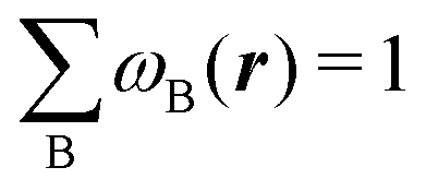
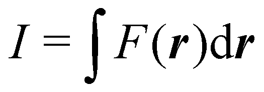 is exactly given by a sum of atomic contributions
 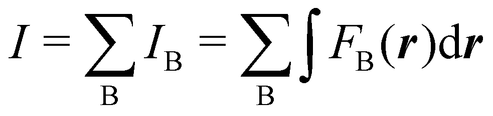 as long as FB(r) = ωB(r)F(r), and the ωB(r) weights satisfy eqn (1). If F(r) = ρ(r) this procedure divides the total electron density into atomic densities.
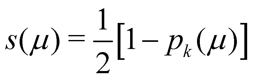 with pk(μ) = p(pk−1(μ)) and p1(μ) = (3/2)μ − (1/2)μ3. A small value of k, say k = 1, gives a slow decrease of s(μ) as we move away from the nucleus A, and k → ∞ provides again the original exhaustive partition. In general, the choice k = 3 is close to optimal and quite appropriate. The equal-atomic-size Becke's partition of R3 ends by defining
 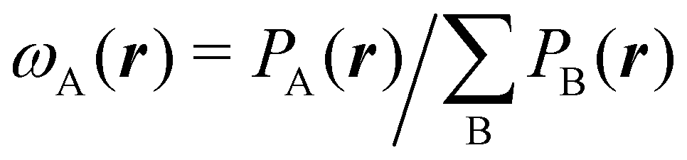 through stockholder sharing, which automatically satisfies eqn (1). To account for the different atomic sizes, Becke replaces μAB by a new coordinate νAB = μAB + aAB(1 − μAB2) in the definition of pk, where |aAB| ≤ 1/2. The plane that bisects the AB internuclear axis in the original recipe is displaced towards center A or towards center B for positive or negatives values of aAB, respectively. Requiring that any point located in that plane (i.e. with νAB = 0) has rA/rB = RA/RB, where RA and RB are Bragg–Slater radii of both atoms, leads to aAB = uAB/(uAB2 − 1), where uAB = (χAB − 1)/(χAB + 1) and χAB = RA/RB. When aAB falls outside the |aAB| ≤ 1/2 range, Becke simply assigns the corresponding endpoint value to it.
 , which is the analogous to Becke's s(μ) function. Köster et al. choose a = 0.7. The different definition of q1 depending on the value of μ dramatically reduces the CPU time required to construct the integration grids.
 . In other words
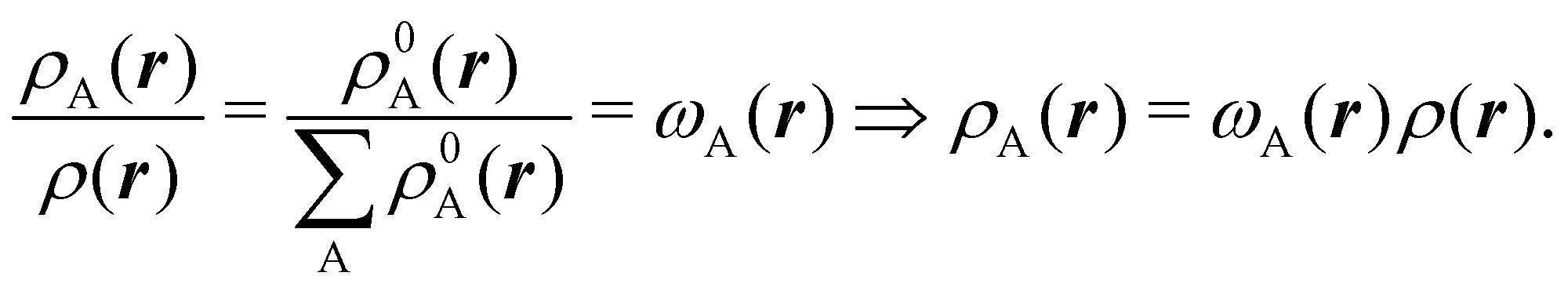
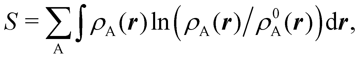 so that these ρA(r)'s best preserve the information contained in the reference ρ0A(r)'s. This property places Hirshfeld's and related atoms among the very limited category of atoms-in-the-molecule that satisfy the physical properties or mathematical constraints. We refer the reader to the works of R. Nalewajski regarding the information on theoric treatment of chemical bonding.57 The original Hirshfeld partition exhibits some clear deficiencies. One of them is the strong dependence of the final electron population of the atoms-in-the-molecule (AIM) on the densities of isolated atoms, which is given by
 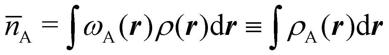 . For instance, the
  and
and  densities of the isolated atoms are used to construct ρ0(r), are very different from those obtained when the ionic references
  and
and  are employed. In the first case, the net charges qNa = ZNa −
  and
and  are used in the method. It seems that Hirshfeld's original method tends to provide atomic charges close to those of the isolated atomic densities, and hence it does not account properly for ionic interactions.
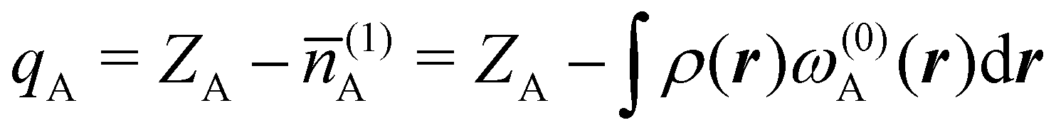 . If qA ≥ 0, a new reference atomic density for A is obtained as
 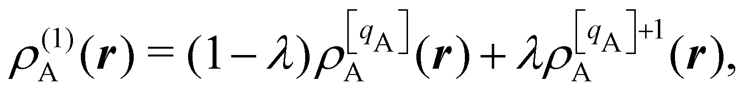 where λ = qA − [qA] and [qA] stands for the integer part of qA. This procedure is nothing but taking the new reference atomic density for atom A as equal to the interpolated value between the isolated densities of ions with net charges [qA] and [qA] + 1. An analogous recipe is used in case that qA < 0. Then, improved weight functions
 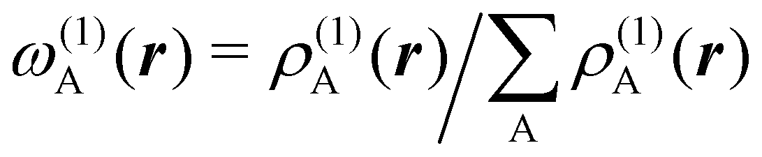 are obtained, and from them new net charges as
 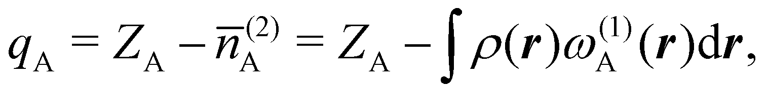 in an iterative process that converges when the qA's in two successive cycles are less than a threshold value. A fast iterative procedure has been developed,59 based on Newton's method, which allows the convergence of the process to be achieved in very few cycles (normally, less than 10). An important point of Hirshfeld-I method is that the final atomic densities ρA(r) yield total electron populations of the atoms-in-the-molecule similar to those provided by the atomic references used to calculate the ωA(r) weights of the last cycle. Better variants that try to improve on still present caveats have also been published, like in the variational Hirshfeld method proposed by Heidar-Zadeh and coworkers.60 We will not extend here any more discussing the progressive improvements of Hirshfeld's method. For further information, we refer the reader to ref. 60. We notice that close to fifty years after Hirshfeld's original idea, the literature is riddled with a number of modified Hirshfeld rules that make it difficult for a non-expert to choose among them. This should be contrasted with QTAIM atoms, that have remained constant over that period of time.
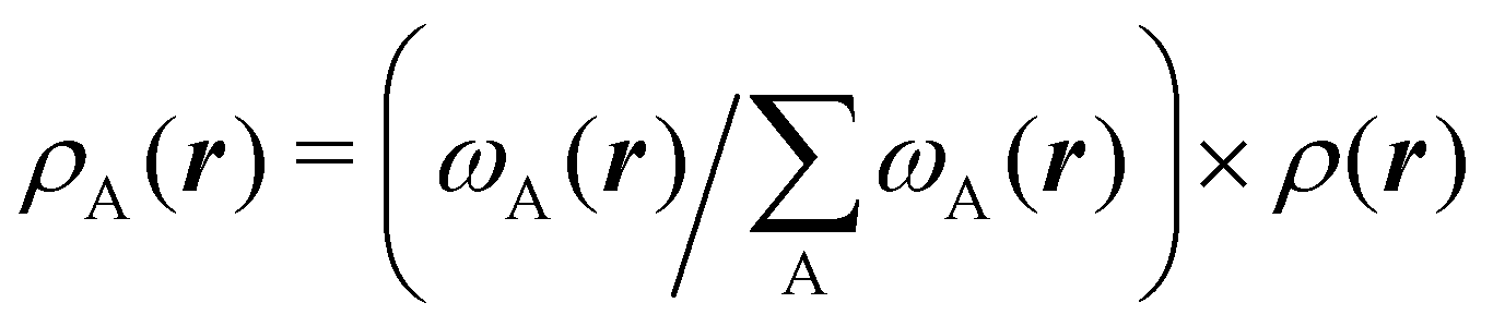
 with
with  , where the ϕ's are nucleus-centered primitive functions, ρij are density matrix elements, and ρAij = ρij, ρAij = 0 or ρAij = (1/2)ρij when both ϕi and ϕj, none of them, or only one of them (ϕi or ϕj) are centered at nucleus A, respectively. Formally similar to Mulliken's atoms are the minimal deformation atoms defined by Fernández-Rico et al.,62 called deformed atoms-in-molecules (DAM) by these authors. They are determined by requiring that each bicentric contributions to ρ(r) has a minimal deformation. In the end, this criterion leads also to
  and
and  where ρAij takes the same values as in Mulliken's atoms, except when only ϕi or ϕj is centered at A, in which case ρAij = ρij if the function centered at A is the one with the largest exponent, and zero otherwise.
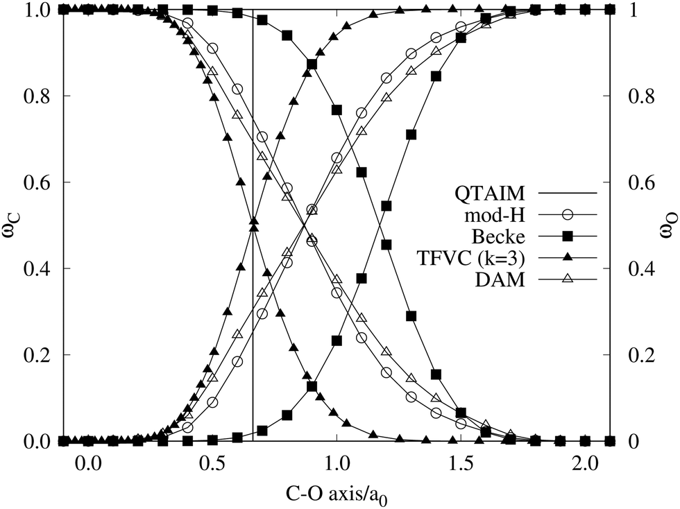
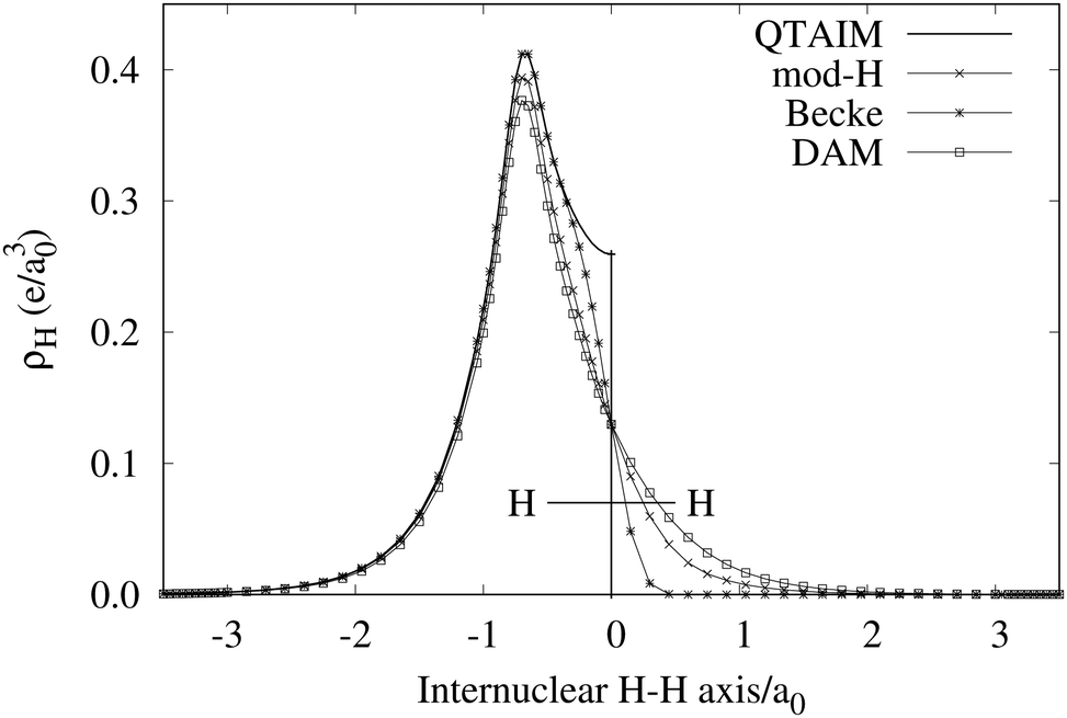
 as well as the interelectron repulsion
 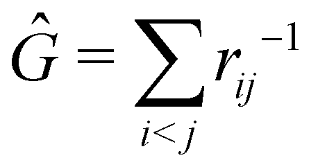 operators. Defining the nth order reduced density matrix (nRDM) (in McWeeny's normalization convention),63 as
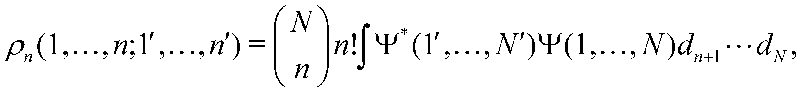
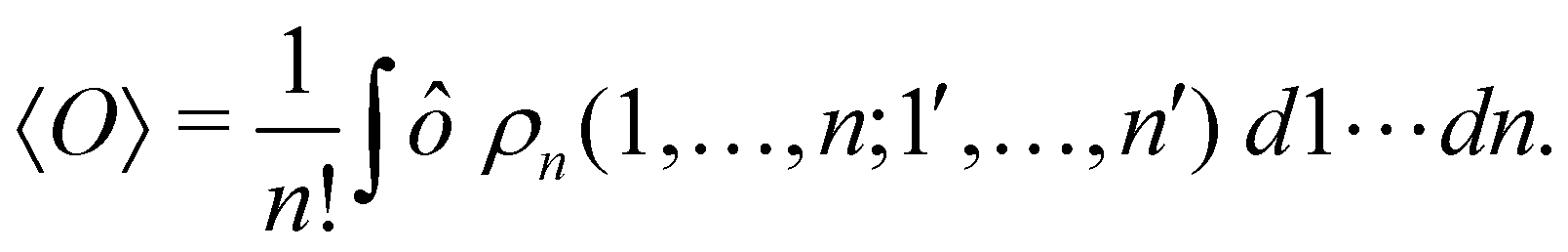
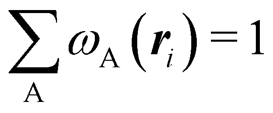 term for each electron coordinate, we arrive at a general atomic partition of 〈O〉:
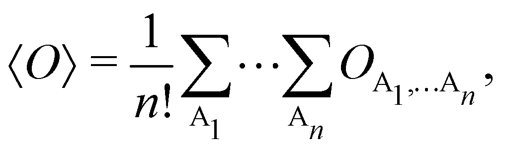
 .
.
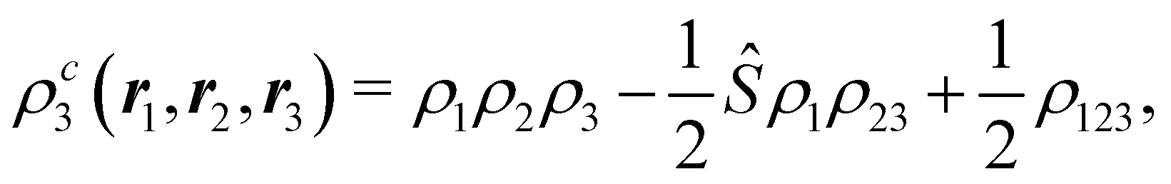
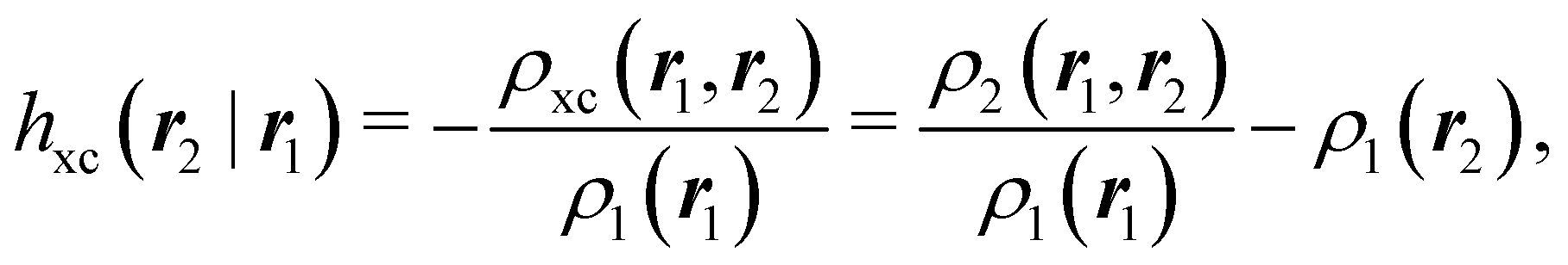


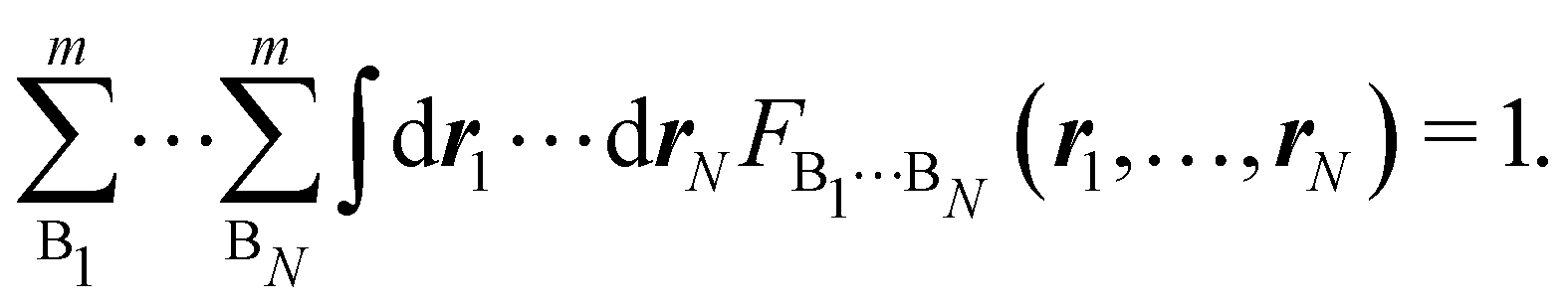
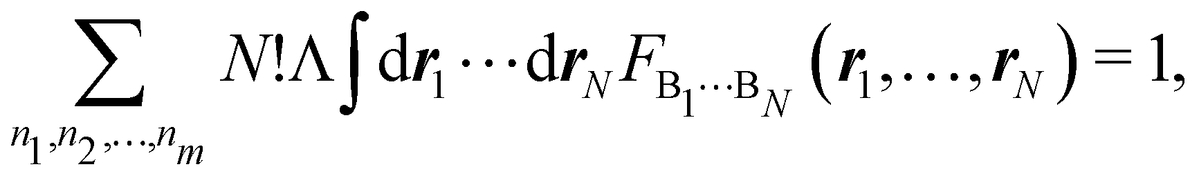


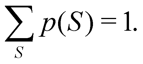
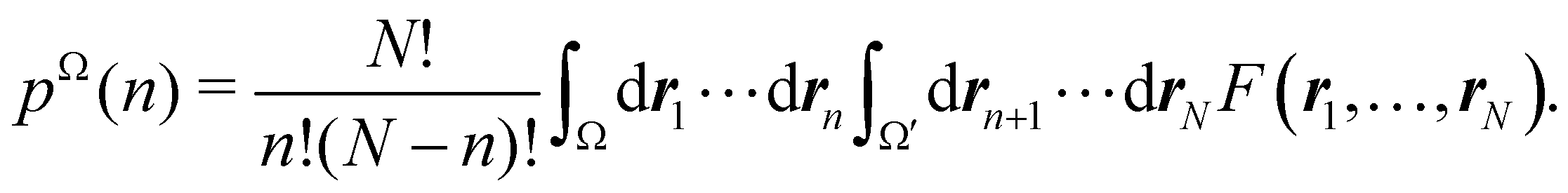

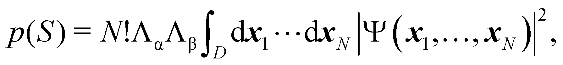


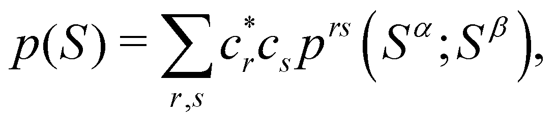

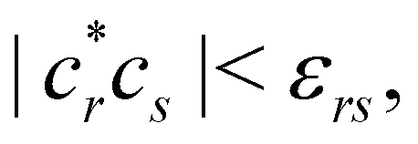 where εrs is another (small) threshold value.
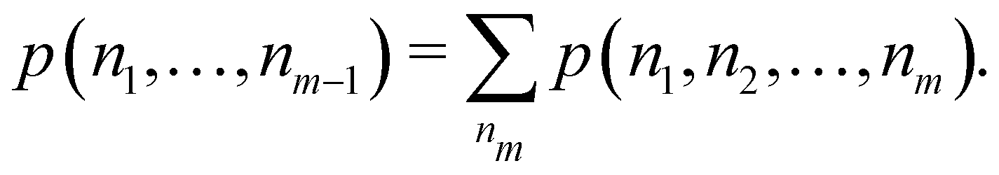


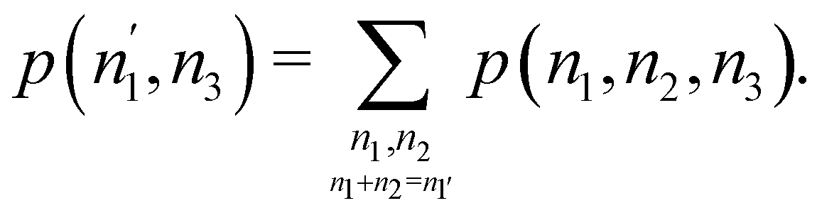
 whose meaning is obvious: we simply multiply each possible value of the number of electrons in Ω(n) by its probability of occurrence (pΩ(n)) and carry out the sum for all ns. This value coincides with that obtained by integrating in R3 the density of the fragment,
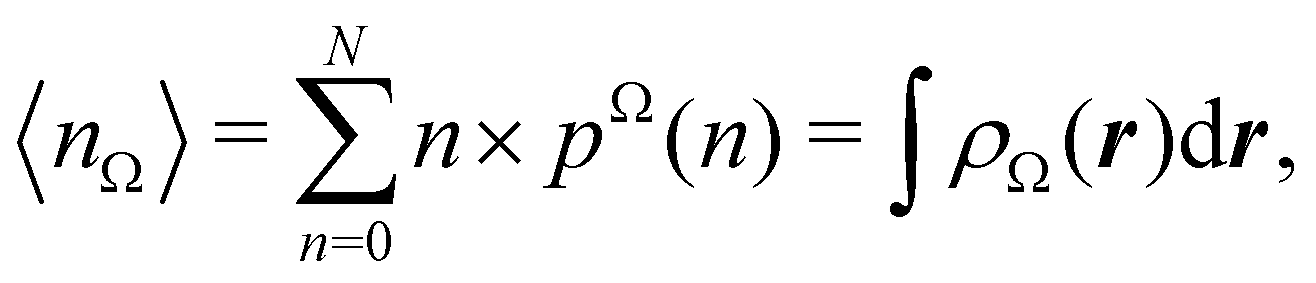
 . The sum over A extends to all the atoms that belong to Ω. In non-fuzzy partitions (in the QTAIM, for instance), the integral in eqn (35) amounts to integrating the full density ρ(r) over the Ω region:
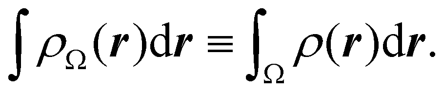
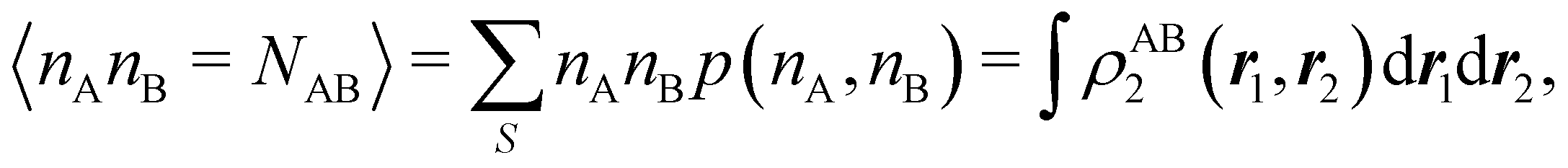
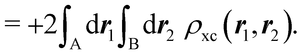
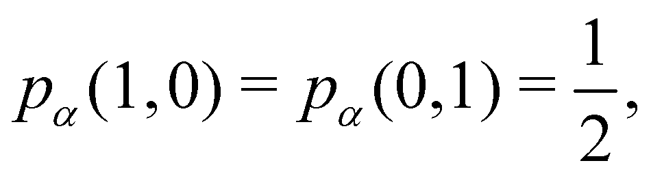 and the same happens with the β electron,
 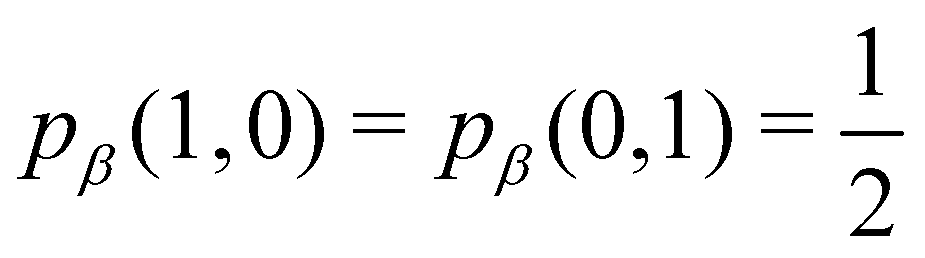 . According to eqn (27), the spin-resolved EDF consists of four equal probabilities; namely
  . The sum of the first two is the spinless probability of finding one electron in A and the other in B (p(1,1)), regardless of their spin, and the third and fourth are the probabilities of finding both electrons in A (p(2,0)) and B (p(0,2)), respectively. Eqn (35) correctly predicts that each atom has on average one electron, 〈nA〉 = 〈nB〉 = 1. However, eqn (38) gives δAB = 1 at any RAB, which is clearly wrong and highlights the well-known dissociation problem of the Hartree–Fock model when the two resulting fragments are open shells. A minimum of two determinants are necessary to correctly dissociate dihydrogen. A complete active space calculation with two electrons in two spin–orbitals (CAS[2,2]), with wavefunction Ψ = c1|σg
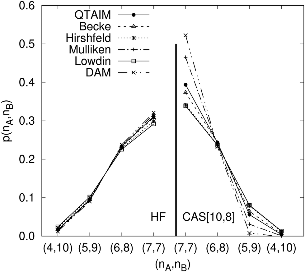
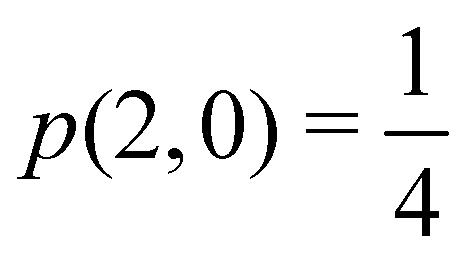 or
or 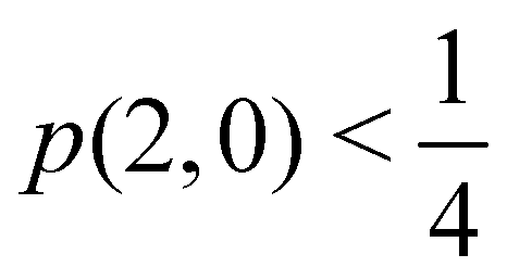 for single- and multi-determinant descriptions, respectively. These results can be immediately extended to the SD case when both fragments are dissimilar. Let π and 1 − π be the probabilities that a first electron of an α–β electron pair is in A (p(A) = π) or B (p(B) = 1 − π), respectively. Since both electrons on a SDW are independent and indistinguishable, we will have p(2,0) = π2, p(0,2) = (1 − π)2, and p(1,1) = 2π(1 − π). To generalize these expressions to the correlated case, we can reason through a Bayesian analysis as follows.106 Provided that one of the electrons is in A, the probability that the second one is in B is
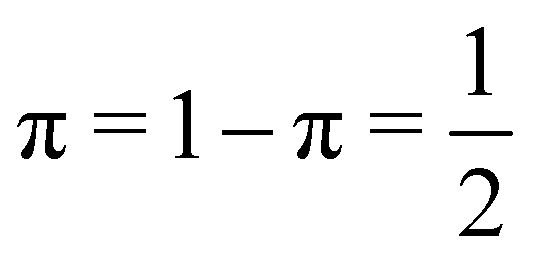 , and p(1,1) = 1 for f = 1.
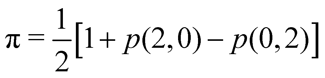 .
.

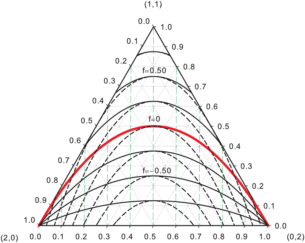

 much smaller than 1.0. The π value for the N–H bond is considerably larger than 0.5, which indicates a clear polarization towards the nitrogen atom, as it is evident if we compare the p(2,0) and p(0,2) values: if one takes an infinite number of snapshots of the N–H bond, 48% of the time both electrons will lie within the N region. The two electrons of these N–H bonds are positively correlated (fi < 0), although we suspect that the value of fi is not very significant in this case, and that it simply absorbs other electronic delocalizations that have not been taken into account in our simple bonding model. Finally, we should notice in the final part of Table 3 that the approximate δAB's are quite similar to the exact ones, particularly for N–H bonds. In the table, N2–H3 and N1–H4 refer to the hypothetical bonds between each N atom and the H atom farthest from it. The exact δAB for them are close to 0.0, which justifies that we have not assumed their existence in our model. The same happens with the hypothetical bond between the two H atoms.

 and ρ2(r1,r2) are 1RDM and the 2RD, respectively, ĥ(r1) is the monoelectronic part of the electronic Hamiltonian as a function of the coordinates of electron 1, while r12 represents the distance between electrons 1 and 2 and Vnn is the internuclear repulsion. Finally, EAself and EABint represent the energy terms which contain particles (i) in only one basin A or (ii) in two different basins A and B, respectively, and are known as the atomic self-energy of atom A and the interaction energy between atoms A and B, respectively. Eqn (53) represents the basis of the Interacting Quantum Atom (IQA) energy partition.14,70
 so that
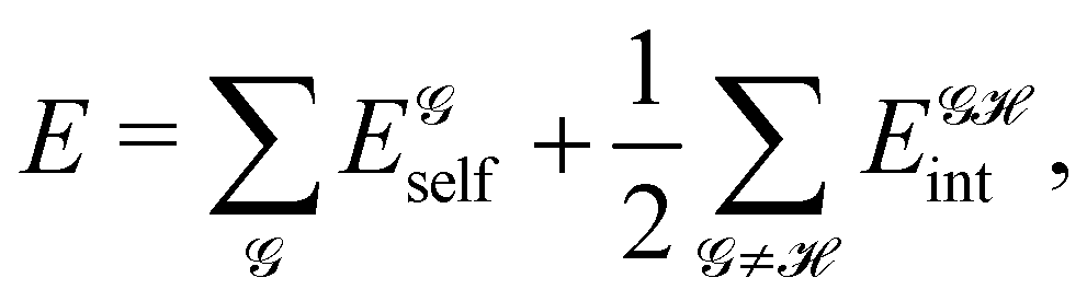
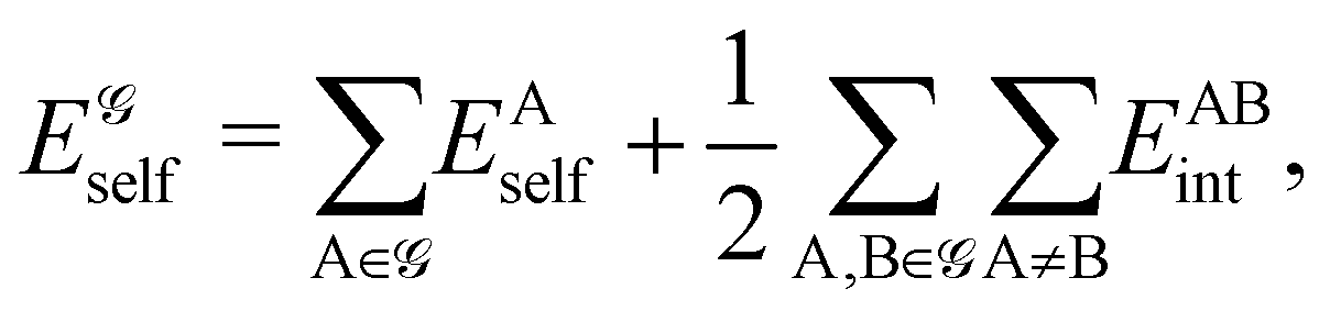
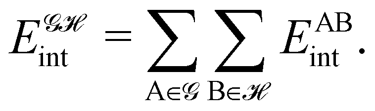
 can also be divided in Coulombic and exchange–correlation contributions,
  and
and  in a similar fashion to EABint in eqn (57). This ability of the IQA approach to provide chemically intuitive answers at different granularities allows for a relatively easy way to compare it to other energy decomposition methods. The other way around is not so obvious. We refer the reader to specific publications on the subject for further information.121,122
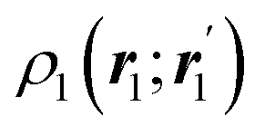 and ρ2(r1,r2) are not attainable via Kohn-Sham Density Functional Theory (KS-DFT), it is possible to divide the KS-DFT electronic energies using scaling techniques as suggested in ref. 123 and 124. Taking into account the popularity of the KS-DFT in modern computational chemistry, this pragmatic strategy has reinforced the applicability and interest of IQA. However, the relatively-high computational cost of IQA is the major inconvenience that remains for its widespread use. This situation, which occurs because the IQA terms involve the integration of scalar fields over very irregular regions, is aggravated for correlated scalar fields
  and ρ2(r1;r2). We expect that such calculations could be accelerated by introducing carefully-controlled approximations, as found in the case of the partition of MP2 correlation energies using effective two-electron matrices,125 which reduces in ∼ 80% of the computational cost for double- and triple-ζ basis sets. More considerable reductions in computer time may result for larger basis sets.
 interactions as well as their covalent and ionic contributions. For instance, the stabilizing role of the H⋯H interaction proposed by Matta and coworkers143 has been the subject of considerable debate.144,145 Several IQA studies146–148 have confirmed the attractive character of this interaction. In like manner, the IQA energy partition and other EDAs have been exploited to determine that the CH⋯HC interactions in the “in–in” conformation of ortho-xylene are also attractive.149 Therefore, the larger stability of the “out–out” conformer is due to other factors which include charge delocalization and aromaticity.
 ) supports the kinetic role of SH that is traditionally claimed to play in the competition between SN2 and E2 reactions.156 On the other hand, the geometric and electronic deformation of a diene/dienophile helps to understand the origin of the endo–exo preference in prototypical Diels–Alder reactions157 while the atomic IQA decomposition of the IRC profiles explains the synchronous or asynchronous character of the polar Diels–Alder reactions.126 Focusing also on the proper fragment quantities, the IQA study of the bifunctional catalysis played by water clusters158 shows how water monomers encompassing the reaction between SO3 and H2O to yield H2SO4 mitigate the changes in chemical bonding across the rate-limiting step of the process, thereby reducing the activation energy as more water molecules are included in the system. Similar results are obtained for the hydrolysis of oxyrane and its methyl derivatives in neutral water.159
 configuration (Fig. 7). Also of particular interest may be the relevant applications on molecular crystals, like the detailed characterization166 of the polymorphism in succinic acid crystals or the assessment of noncovalent contacts within selected hydrogen storage materials KN(CH3)2BH3 and LiN(CH3)2BH3.167 Other materials that have been examined with the IQA energy partition are the donor–acceptor charge–transfer tetrathiafulvalene–tetracyanoquinodimethane cocrystals.168 More specifically, the IQA approach unveils the stabilizing (or destabilizing) character of C⋯S, Csp3–H⋯S and S⋯S interactions within these systems. Likewise, the IQA method characterizes Cl⋯S, Cl⋯Cl and O⋯Cl contacts in trimers of 2-chloro-5-methoxy-naphtho[1,2-d]thiazole, used as an archetype in the study of organic semiconductors.169 Actually, a specific implementation of the IQA method for the study of crystals has been developed and successfully tested in crystals with different types of bondings.170 Eventually, this enhanced IQA methodology will permit to tackle interesting and challenging problems, such as the origin of different stabilities of crystalline phases (e.g. graphite versus diamond).
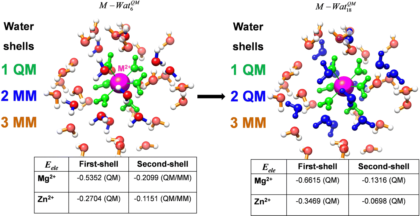

 , where α runs over the nuclei and Z denotes the nuclear charge, has been added to the electron density ρ to define a total (electronic plus nuclear) charge density, ρt(r) = ρn(r) − ρ(r). We now recall that the covalent bond order, as measured by the delocalization index δAB, given by eqn (39) which, apart from the r12 interelectron distance, is just a scaled EABxc. Using a bipolar expansion, which is always convergent unlike the more commonly found multipolar expansion,226 it has been shown71 that both the covalent and ionic terms can be written as Taylor series in which the leading terms are


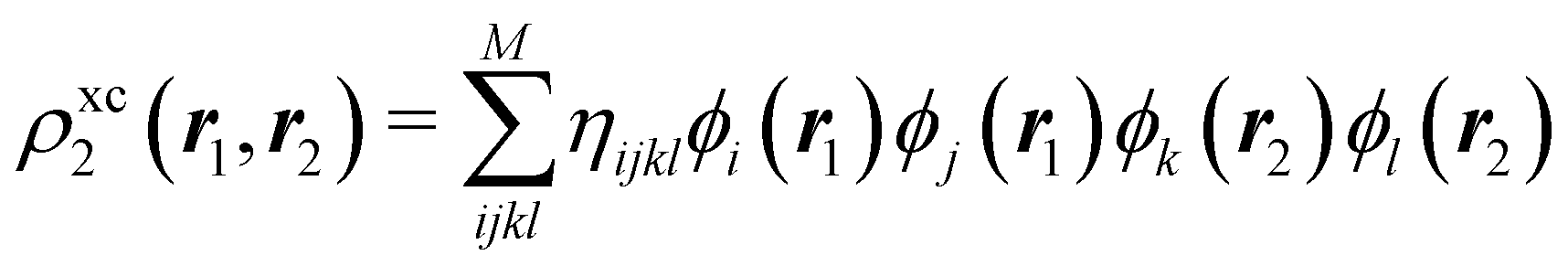

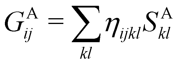 . The diagonalization of GA/2 = GAα = GAβ leads to a set of M DAFH MOs ϕAi(r) and their corresponding occupation numbers nAi. The DAFH MOs of highest occupancy for the methanol molecule and their occupation numbers at the CCSD(T)//cc-pVDZ level are provided in Fig. 12. These are well-defined functions obtained at any level of theory that preserve conventional chemical wisdom and that are invariant under orbital tranformations of the underlying wavefunction. Notice how close to two the propulations are, much as in NBO analyses, without the need of the involved and some times ad hoc transformations that lead to natural bond orbitals.
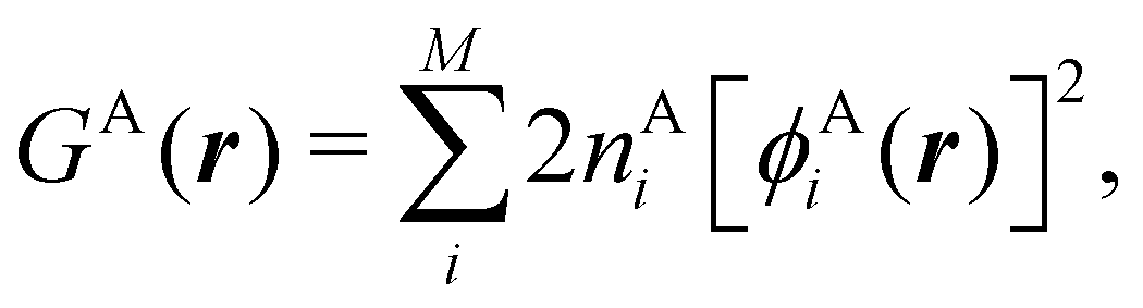
 , the average number of electrons in A. Given that
  , we also have
 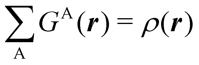 . From eqn (39), (65) and (66), the delocalization index between A and B, δAB, is given by248
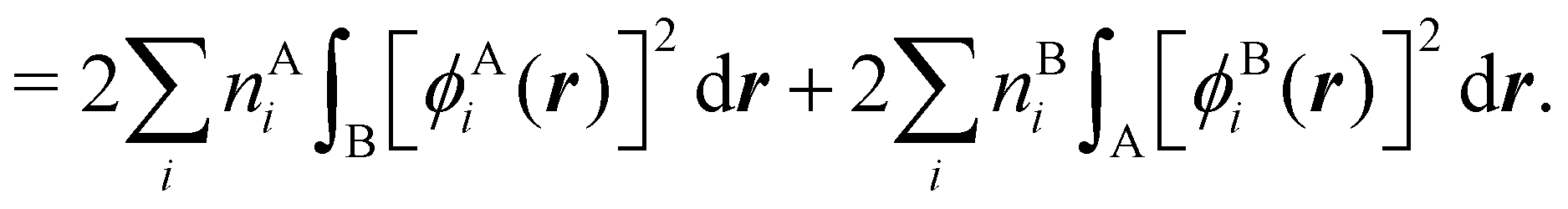
 . δAB takes a simpler form when the sum of fragments A and B exhaust the system (A∪B = R3). Then, the first integral in eqn (68) is equal to 1 − sAi, where
  , and the second becomes 1 − sBi, where
  so δAB can be written as
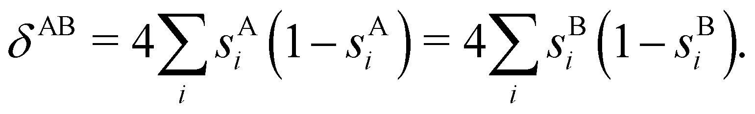
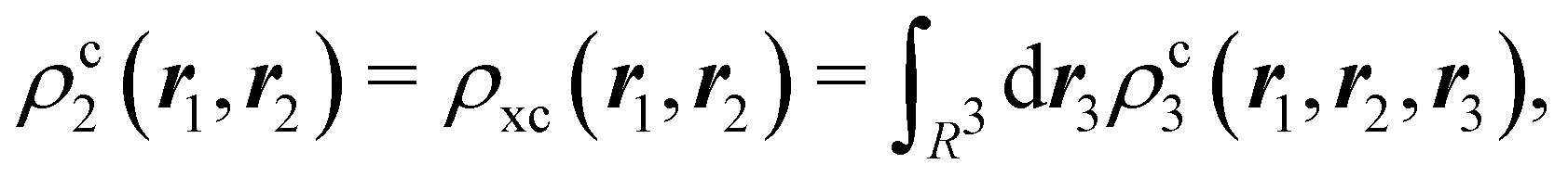
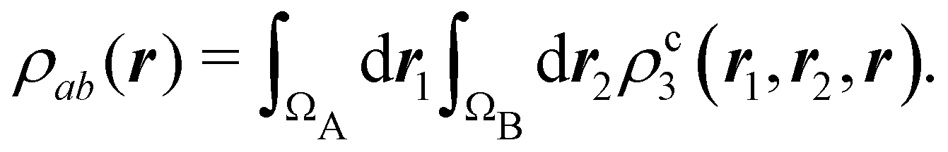

 , and each ψabi(r) is normalized, the nabis obey the sum rule
  . Thus, 2 × nabi is the contribution of ψabi(r) to the bond order between A and B, and each ψabi itself defines a two-center natural adaptive orbital (NAdO). This means that two-center NAdOs induce a one-electron decomposition of any two-center delocalization index.

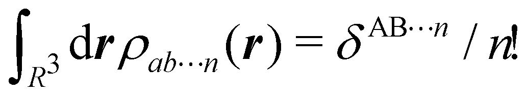 and the ψab⋯ni(r)'s are again normalized, the sum rule is now
 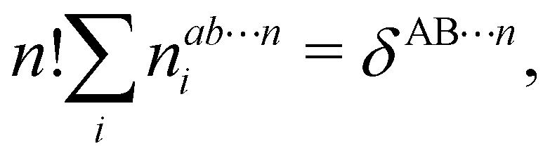 than can be taken as an n-center delocalization index. When n = 1, the generalized density ρa(r) coincides with the DAFH function GA(r) defined in the previous subsection, and the 1-center NAdOs ψai(r) and their eigenvalues nai's are equal to twice the DAFH occupancies (2nAi) and DAFH MOs ϕAi(r).
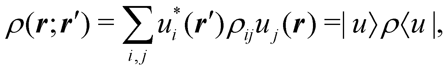
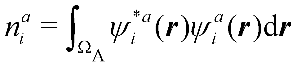 .
.