DOI:
10.1039/D4FD00035H
(Paper)
Faraday Discuss., 2024,
254, 429-450
Rapidly convergent quantum Monte Carlo using a Chebyshev projector
Received
25th February 2024
, Accepted 1st May 2024
First published on 2nd May 2024
Abstract
The multireference coupled-cluster Monte Carlo (MR-CCMC) algorithm is a determinant-based quantum Monte Carlo (QMC) algorithm that is conceptually similar to Full Configuration Interaction QMC (FCIQMC). It has been shown to offer a balanced treatment of both static and dynamic correlation while retaining polynomial scaling, although application to large systems with significant strong correlation remained impractical. In this paper, we document recent algorithmic advances that enable rapid convergence and a more black-box approach to the multireference problem. These include a logarithmically scaling metric-tree-based excitation acceptance algorithm to search for determinants connected to the reference space at the desired excitation level and a symmetry-screening procedure for the reference space. We show that, for moderately sized reference spaces, the new search algorithm brings about an approximately 8-fold acceleration of one MR-CCMC iteration, while the symmetry screening procedure reduces the number of active reference space determinants with essentially no loss of accuracy. We also introduce a stochastic implementation of an approximate wall projector, which is the infinite imaginary time limit of the exponential projector, using a truncated expansion of the wall function in Chebyshev polynomials. Notably, this wall-Chebyshev projector can be used to accelerate any projector-based QMC algorithm. We show that it requires significantly fewer applications of the Hamiltonian to achieve the same statistical convergence. We benchmark these acceleration methods on the beryllium and carbon dimers, using initiator FCIQMC and MR-CCMC with basis sets up to cc-pVQZ quality.
1 Introduction
Quantum Monte Carlo (QMC) methods have long provided a powerful alternative to conventional electronic structure methods, by generating high accuracy results at a fraction of the cost of standard approaches. The combination of Variational Monte Carlo (VMC)1,2 and Diffusion Monte Carlo (DMC)3–5 has become a significant benchmarking approach in many areas of electronic structure,6–10 but it is limited by the need to provide an approximate nodal structure to avoid collapse onto bosonic solutions. Fermionic Monte Carlo methods11,12 have since been developed which act directly in the anti-symmetrised Hilbert space of the electronic structure problem, thereby removing the potential for bosonic solutions a priori.
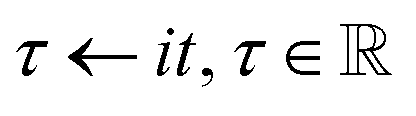
First introduced in 2009 by Booth et al.,11 full configuration interaction quantum Monte Carlo (FCIQMC) can be variously described as a stochastic power iteration algorithm or an iterative solution to the imaginary time Schrödinger’s equation. Here, we give a brief summary of the theoretical underpinnings of FCIQMC by taking the latter view. By applying a Wick rotation,13 , to the time-dependent Schrödinger’s equation
  , one obtains the imaginary time Schrödinger’s equation:
| | 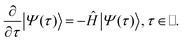 | (1) |
It can be formally integrated to give
| | | |Ψ(τ)〉 = e−τ(Ĥ−S)|Ψ(0)〉, | (2) |
with
S being the constant of integration, also known as the ‘shift’.
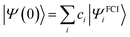
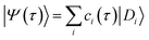
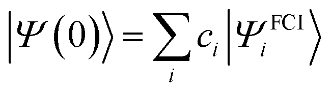
The reference wavefunction |Ψ(0)〉, commonly a Hartree–Fock (HF) solution, can be expanded in the eigenbasis of the full Hamiltonian, {|ΨFCIi〉}, leading to
| | 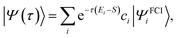 | (3) |
with {
Ei} being the eigenspectrum of the full Hamiltonian and
. We can see that, if
S =
E0, in the limit of
τ → ∞, we obtain the ground state of the full Hamiltonian.
By discretising the projector in eqn (2) and further applying the first-order Taylor series expansion, we obtain the ‘master equation’ of FCIQMC:
| | | |Ψ(τ + δτ)〉 = [1 − δτ(Ĥ − S)]|Ψ(τ)〉. | (4) |
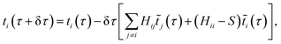
This equation can be projected onto the different determinants in the Hilbert space to give
| | | 〈Di|Ψ(τ + δτ)〉 = 〈Di|Ψ(τ)〉 − δτ〈Di|Ĥ − S|Ψ(τ)〉, | (5) |
which gives an update equation for the corresponding FCI parameters
ci, where
:
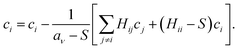
| | 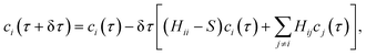 | (6) |
where
Hij = 〈
Di|
Ĥ|
Dj〉. This equation can be viewed as describing the population dynamics of particles placed on the different determinants and may be modelled by a stochastic process composed of three steps:
11
• Spawning: given determinant Di, generate new particles on determinant Dj with probability p ∝ δτHijci(τ).
• Death: given determinant Di, generate new particles on determinant Di with probability p ∝ δτ(Hii − S)ci(τ).
• Annihilation: for a given determinant, cancel out particles carrying opposite signs.
The formulation of CCMC closely matches that of FCIQMC, with the difference that instead of residing on determinants, walkers reside on excitors, ân, defined as ân|D0〉 = ±|Dn〉, where the choice of sign is a matter of convention. Replacing the FCI wavefunction by the coupled-cluster ansatz in eqn (4) and left-multiplying by 〈Di| gives
| | | 〈Di|ΨCC(τ + δτ)〉 = 〈Di|ΨCC(τ)〉 − δτ〈Di|(Ĥ − S)|ΨCC(τ)〉, | (7) |
The coupled-cluster ansatz parametrises the wavefunction with cluster amplitudes in a non-linear fashion. The mapping of CI coefficients to cluster amplitudes can be done by a simple projection, which reveals contributions from multiple clusters. For example, in a CCSD wavefunction (i.e., ![[T with combining circumflex]](https://www.rsc.org/images/entities/i_char_0054_0302.gif) = 1 + 2):
= 1 + 2):
| | | 〈Dabij|eD0〉 = tabij + taitbj − tbitaj, | (8) |
with the negative sign arising from the fact that
â†bâiâ†aâj = −
â†aâiâ†bâj, due to the anti-commutation relations of the second-quantised creation and annihilation operators.
14 Terms like
tabij are known as non-composite cluster amplitudes, and the rest as composite cluster amplitudes. Here we make the approximation that composite clusters have much smaller contributions than non-composite ones, their changes will be negligible per time step, and hence we can remove the

contributions on both sides to write
| |  | (9) |
Compared to FCIQMC, an additional step needs to be performed for each Monte Carlo iteration: the sampling of the exponential ansatz. For
Nex total walkers, also called excips in CCMC,

clusters are formed randomly by combining present excitors according to specific biasing rules.
15
Finally, the intermediate normalisation16 of the wavefunction is redefined to give the CCMC ansatz:
| | | |ΨCCMC〉 = N0e/N0|D0〉, | (10) |
which introduces the reference population as a new independent variable, solving the problem that
eqn (7) does not lead to a viable update equation for 〈
Di| = 〈
D0|.
A multireference formulation of the CCMC algorithm (MR-CCMC)17 has been implemented, retaining a single-reference formalism, in common with the so-called SRMRCC methods in ref. 18. The flexibility of the CCMC algorithm allows this multireference approach to be implemented with minimal code changes to the single-reference algorithm, bypassing what would be a challenging process in deterministic methods. Essentially, for a coupled-cluster truncation level P, the algorithm allows any number of determinants to become a ‘secondary reference’, stores excitors that are within P excitations from any references (instead of just the HF determinant), and allows clusters to form that are within P + 2 excitations from any reference. The set of references is commonly known as the model or reference space. To summarise, the algorithmic modifications relative to single-reference CCMC are:
• Store all the secondary references in some searchable data structure, and additionally store the highest excitation level from the reference determinant among the secondary references, kmax.
• Cluster expansion: allow clusters with an excitation level of up to kmax + P + 2 to form, instead of P + 2 in the single-reference case. Discard those that are not P + 2 excitations away from some reference determinant.
• Spawning: for a randomly generated spawnee (i.e., 〈Dj|), check that it is within P excitations of any secondary references.
• Cloning/death: allow death on excitors that are within P excitations from any secondary references.
While this MR-CCMC method can treat systems that conventional single-reference CC struggles with, this comes at an increased computational cost. Comparing contributor excitation levels to all references becomes expensive as the number of references grows, particularly when the contributor turns out to lie outside of the desired space. Therefore, non-trivial computational effort is expended on attempts that will not contribute to the overall estimators and propagation, while also making successful steps more expensive than their single-reference equivalents.
In the rest of this paper, we will first introduce the wall-Chebyshev projector, which can replace the traditional linear QMC projector, and show that it can be applied to (MR-)CCMC and FCIQMC to reduce the number of times the Hamiltonian needs to be applied to reach statistical convergence, thereby reducing the computational cost. MR-CCMC in particular is a convenient testing ground for this new approach, as it can treat systems in a variety of correlation regimes, preserving polynomial scaling with system size, which makes calculations significantly cheaper than their FCIQMC counterparts. However, in order for the MR-CCMC algorithm to be able to take full advantage of the speed-up provided by the wall-Chebyshev projector, we also introduce a suite of specific modifications to the MR-CCMC algorithm that accelerates the handling of the reference space. We apply the resulting algorithm to several traditional benchmark systems to investigate the performance enhancements due to the proposed algorithmic improvements.
2 The wall-Chebyshev projector
2.1 Motivation and theory
In common projector-based QMC methods, including FCIQMC and CCMC, a linear projector (eqn (4)) is used. The first-order Taylor expansion turns out to be a very reasonable approximation, since we demonstrate in Appendix A.1 that there is no benefit whatsoever in going to higher orders of the Taylor expansion of the exponential projector. However, this does not mean that one cannot devise more efficient projectors. An example is a projector based on a Chebyshev expansion of the wall function, which was first proposed in ref. 19 in the context of a deterministic projector-based selected CI algorithm.
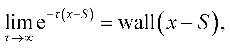
The wall function is given by
| |  | (11) |
and is physically motivated as the infinite time limit of the exponential projector:
| |  | (12) |
which can map any trial wavefunction |
Φ0〉 to the exact ground state |
Ψ0〉, if 〈
Φ0|
Ψ0〉 ≠ 0 and
E0 ≤
S <
E1.
While a Taylor series expansion does not exist for the discontinuous wall function, an expansion in Chebyshev polynomials, like a Fourier expansion, is trivial. The Chebyshev polynomials of the first kind, defined as Tn(cos(θ)) = cos(nθ), form an orthogonal basis (with metric (1 − x2)−1/2) for functions defined over x ∈ [−1,1]:
| |  | (13) |
To facilitate the following discussion, we define the spectral range, R, of a Hamiltonian as R = EN−1 − E0, where Ei is the ith eigenvalue of the full Hamiltonian and N is the size of the Hilbert space. Furthermore, our energy range ε ∈ [E0,EN−1] requires the application of an affine transformation to the Chebyshev polynomials:
| |  | (14) |
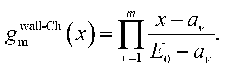
We show in Appendix A.2 that the mth-order Chebyshev expansion of the wall function is
| |  | (15) |
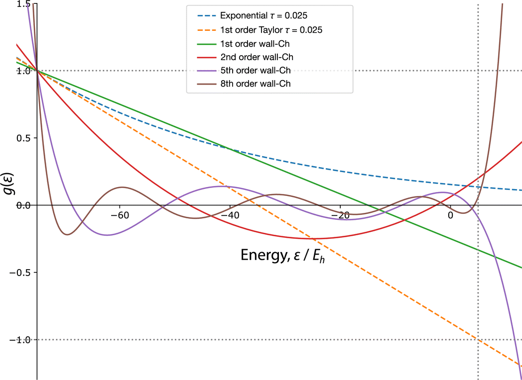
For illustration purposes, we plot several orders of Chebyshev expansion in Fig. 1, where we can also observe the monotonic divergence to +∞ for ε < E0. The other tail also diverges to ±∞ depending on the parity of the order m.
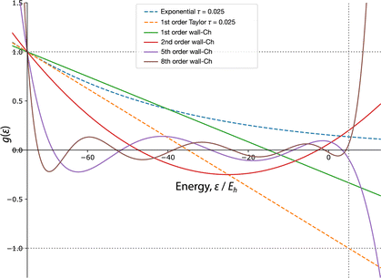 |
| | Fig. 1 The Chebyshev expansions of the wall function in an arbitrary range of [−75,5], compared to the linear projector with the maximal time step of δτ = 0.025, and its corresponding exponential projector. | |
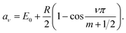
In this instance, the nodes of eqn (15) are analytically known (see derivation in Appendix A.2) as
| |  | (16) |
This allows us to decompose the
mth-order projector into a product of
m linear projectors, each with their own weight that ensures
gwall-Chm(
E0) = 1:
| |  | (17) |
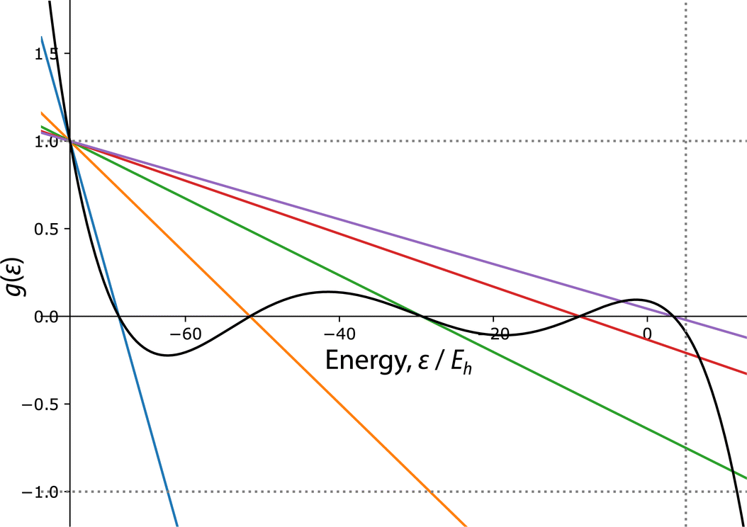
A decomposition for a fifth-order Chebyshev expansion of the wall function can be seen in Fig. 2.
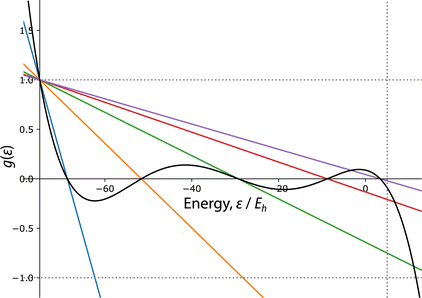 |
| | Fig. 2 The fifth-order Chebyshev expansion of the wall function, shown here to decompose into a product of 5 linear projectors, each with their own effective time steps. | |
2.2 Application to FCIQMC and CCMC
In FCIQMC and CCMC, the lowest eigenvalue estimate is the shift, S, and the upper spectral bound can be a constant, estimated from the Gershgorin circle theorem20 as| |  | (18) |
where the sum is over all determinants connected to the highest determinant (singles and doubles), and the ‘′’ restricts it to j ≠ N − 1.
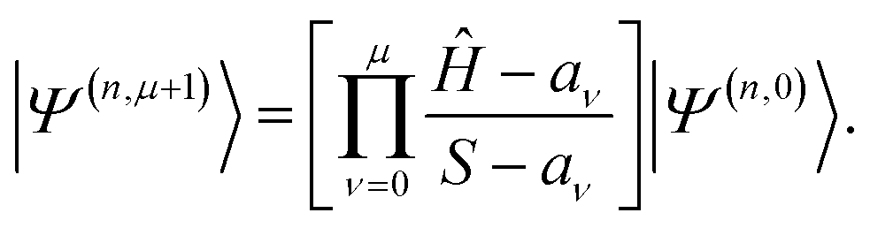
The action of the wall-Chebyshev projector on |Ψ(n,0)〉 = [gwall-Ch(Ĥ)]n|Φ〉 is
| | | |Ψ(n+1,0)〉 = gwall-Ch(Ĥ)|Ψ(n,0)〉, | (19) |
which gives the wavefunction after
n + 1 applications of the projector. We can additionally define the ‘intermediate’ wavefunctions as
| | 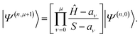 | (20) |
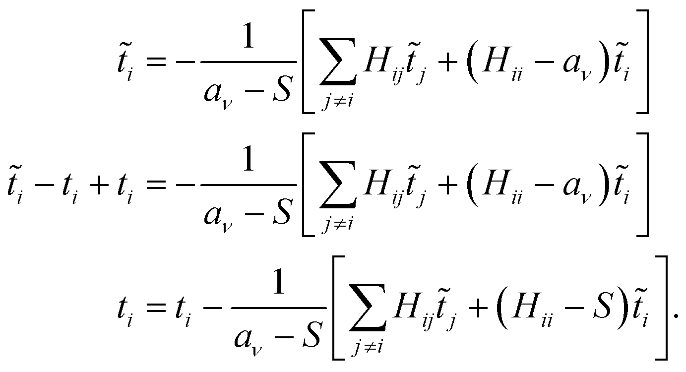
We are now ready to derive the update equations for FCIQMC and CCMC. We start with the slightly more involved derivation for CCMC. Projecting these intermediate wavefunctions onto determinants, we have
| | 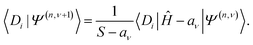 | (21) |
It is important now to distinguish between
![[t with combining tilde]](https://www.rsc.org/images/entities/i_char_0074_0303.gif) i
i, the projection of a wavefunction onto determinant
Di, and the corresponding excitor amplitude,
ti, with the former including unconnected (‘composite’) contributions. At convergence,
| | 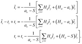 | (22) |
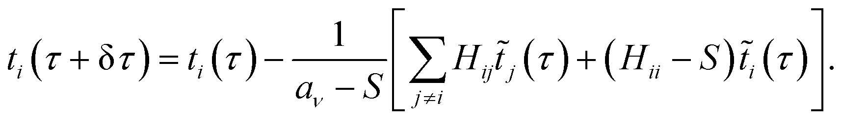
We may now convert the last equation into an update step,
| |  | (23) |
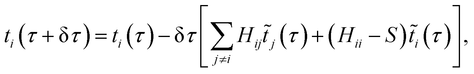
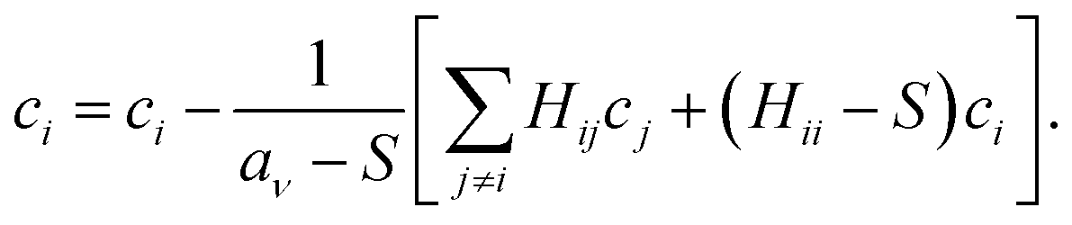
Comparing with the original update equations, which are given by
| |  | (24) |
we reach the conclusion that the necessary modifications are:
(1) Setting δτ = 1
(2) Applying the m constituent linear projectors in the mth-order wall-Chebyshev projector. For linear projector ν ∈ {0, …, m − 1}, scale Hamiltonian elements in spawning and death by 1/(aν − S) (‘Chebyshev weights’).
The same analysis can be performed on FCIQMC, without the complication of composite amplitudes, to obtain a similar set of update equations:
| |  | (25) |
In terms of implementation, the two sets of update equations are nearly identical, and can share the same code in large parts.
Analysis of the asymptotic rate of convergence (see Appendix A.3) shows that the theoretical speedup of an order m wall-Chebyshev projector relative to the linear projector with largest allowed δτ is (m + 1)/3.19 Due to blooms, the largest δτ is never reached in the conventional propagator, so real speedups are expected to be larger.
2.3 The shift update procedure
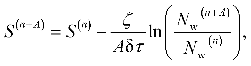
The original shift update equation for CCMC and FCIQMC is given by| | 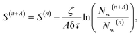 | (26) |
where the update is performed every A time steps, ζ is the shift damping parameter, and Nw is the total number of walkers.
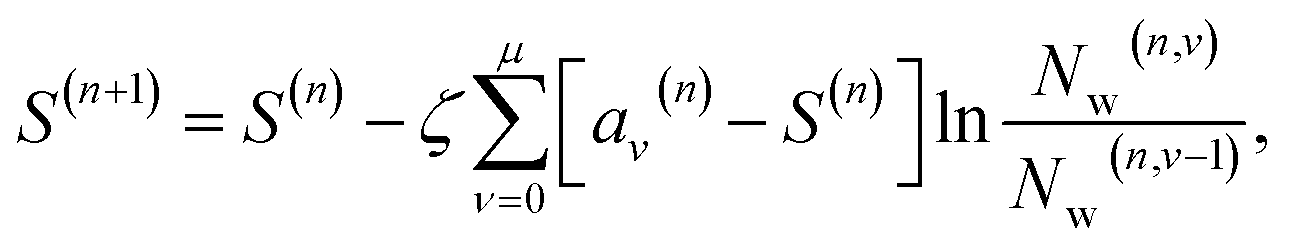
Due to the time step δτ being set to unity, the shift update procedure is expected to become rather unresponsive to the changes in particle population. As a consequence, there can be vastly uncontained spawning, unchecked by the lower-than-expected deaths, resulting in unmanageable population growths. To remedy this, initially, a scaled update procedure was experimented with, setting A = 1:
| |  | (27) |
which seemed attractive as it reduces to
eqn (21) in the first-order case where the sum only contains one term or if all Chebyshev weights are the same. However, this was not successful in reining in the population growth. We believe this is because the intermediate wavefunctions in
eqn (20) are ill-behaved due to being generated by an effective time step potentially larger than
τmax. A series of population changes that start and end at
N(n) and
N(n+1), respectively, can produce very different values of shift update in
eqn (27), and the shift update produced is very sensitive to the unreliable intermediate values. Hence the population information from these intermediate wavefunctions should not be used.
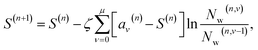
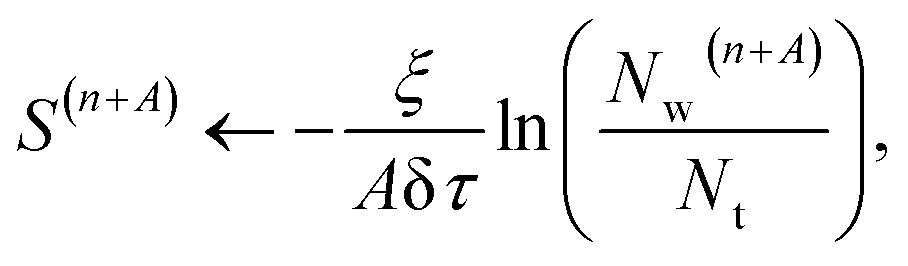
Another procedure that was more successful was to decrease the damping (by increasing ζ) of the shift updates, causing the shift to be more responsive to the changes in populations, which in turn helps stabilise the population. We also found it helpful to use the improved shift update procedure outlined in ref. 21, where an additional term is added to the shift update procedure:
| |  | (28) |
where
ξ is the ‘forcing strength’, and
Nt is the target population. This has the effect of additionally stabilising the population by ‘pinning’ it to the pre-set target population. A further proposal from the same paper, arising from an argument from a scalar model of population dynamics, is for critical damping to be achieved by setting
ξ =
ζ2/4. This is also found to be helpful. Altogether, these modifications result in greatly improved population control and we were able to obtain dynamics that can be used in a reblocking analysis, as shown in
Fig. 7, for example.
In practice, we have also found that with increasing order of Chebyshev projector, a larger target population is usually needed, otherwise the calculation may exhibit a sign-problem-like divergence. This may be attributed to the larger effective time steps that the higher-order projectors use and is documented elsewhere; for example, see Fig. 2 in ref. 22.
3 Accelerating the MR-CCMC algorithm
The MR-CCMC method is a promising candidate for tackling strongly correlated systems at polynomial cost, and represents an economical alternative to the related exponentially scaling FCIQMC method. In this section we detail two algorithmic developments that have greatly accelerated the MR-CCMC calculations in the remainder of the article, and have brought MR-CCMC a step closer to algorithmic maturation.
3.1 Efficient cluster acceptance algorithm
In the spawning step of the MR-CCMC algorithm, we check that a spawnee is within P excitations of any secondary reference. The same check needs to be performed in the death step. The original MR-CCMC algorithm performed a linear scan through the list of secondary references, which is clearly a  operation, where nref is the number of secondary references. The subroutine that decides whether a spawn is accepted is the second most frequently called subroutine in the program, after the excitation generator. Therefore, a linear search in this step can quickly become prohibitively expensive in a moderate to large reference space (nref > 1000, for example). We note that traditional data structures and search algorithms, such as a binary search on a sorted list of secondary references, would not work here, as the definition of ‘distance’ in this case, i.e., excitation-rank, is non-Euclidean. A search algorithm in a general metric space is therefore needed.
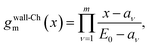
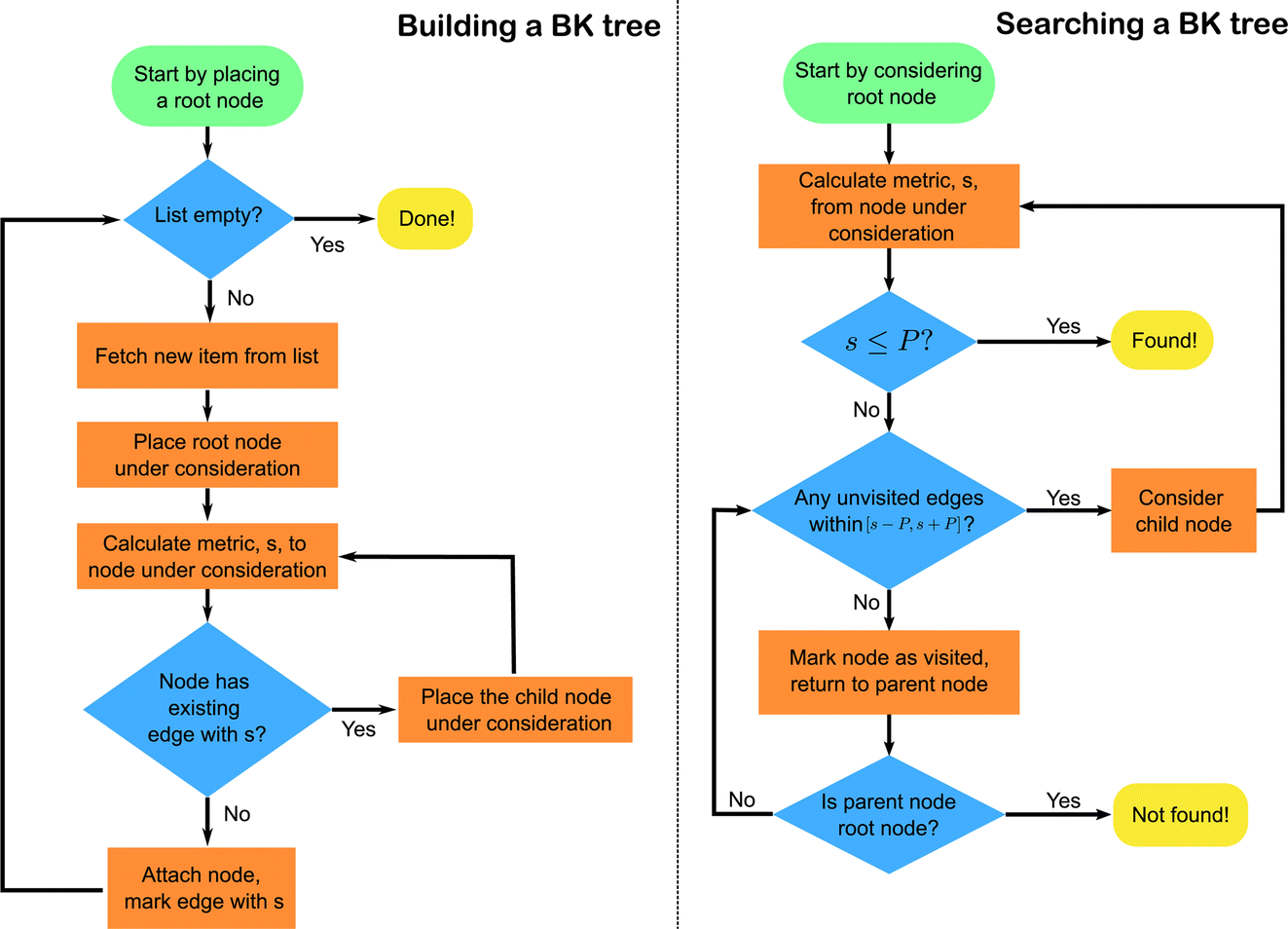
The excitation-rank distance between two Slater determinants is equivalent to half the Hamming distance between the bit strings representing these two determinants, and the Hamming distance is a well-known example of a discrete metric.23 A data structure, known as the BK-tree,24 is particularly well suited for efficient searches in discrete metric spaces. The tree, an example of which is given in Fig. 3, is constructed only once at the beginning of the calculation. Subsequently, the search can be performed in  time using a recursive tree traversal algorithm. The tree construction and search algorithms are pictured in Fig. 4.
 |
| | Fig. 3 The BK tree can conduct efficient nearest-neighbour searches in a discrete metric space, like the excitation rank. In this figure a BK-tree built from 20 arbitrary determinants is shown. The topology of the tree is not unique, and is dependent on the order the nodes were added to the tree. | |
 |
| | Fig. 4 Flowcharts for the building and searching of a BK-tree. | |
3.2 Compression of the reference space
Whereas many classical multireference coupled-cluster (MRCC) methods work with complete active spaces (CAS), the MR-CCMC algorithm as presented here is highly flexible as to the shape of the reference space, and as such can be considered a general reference space method.18 This enables us to consider arbitrary subsets of the CAS as the reference space, and fine-tune the balance between cost and accuracy. One of us has devised a compression method in this vein.25 Here we briefly summarise its main thrust.
Two of us observed17 that for some (ne,no) active spaces, the results of a MR-CCSD calculation using all of the determinants in the active space as references (i.e., a CAS MR-CCSD calculation) is qualitatively very similar to the results of a MR-CCSD…m calculation, where m = n/2, using only the ‘bottom’ and ‘top’ determinants (i.e., the aufbau and anti-aufbau determinant, respectively) of the CAS as the references. We term the latter calculation as ‘2r-CCSD…m’. Using this observation, we aim to algorithmically generate only those determinants that are in the Hilbert spaces of both the CAS MR-CCSD and 2r-CCSD…m calculations, which should provide us with a compressed set of reference determinants that captures the most important determinants in the CAS. It was shown that this set of determinants can be generated by enumerating determinants of up to (m − 2)-fold excitations from the bottom and top determinants.
4 Computational details
In this work we study carbon and beryllium dimers, using MR-CCMC and initiator FCIQMC (i-FCIQMC).26 The first system displays challenging multireference behaviour, requiring an (8e,8o) CAS as the reference space for MR-CCMC, which is large enough to benefit from the techniques presented in Section 3. Overall MR-CCMC and i-FCIQMC calculations are performed in the full space of (12e,28o). The beryllium dimer on the other hand is only moderately multireference, but exhibits weak bonding, with a dissociation energy of only approximately 4 mEh. Accurately describing this behaviour in QMC requires low stochastic noise in the energy estimates. The accelerated convergence provided by the wall-Chebyshev propagator is therefore particularly beneficial in reducing the propagation time required to obtain low-variance estimates. For these systems, Dunning’s cc-pVXZ basis sets are used.27 The required electron integrals are generated by the Psi4![[thin space (1/6-em)]](https://www.rsc.org/images/entities/char_2009.gif) 28 and PySCF29 packages. The electron integrals are generated in the D2h point-group symmetry and transformed into the basis of
28 and PySCF29 packages. The electron integrals are generated in the D2h point-group symmetry and transformed into the basis of ![[L with combining circumflex]](https://www.rsc.org/images/entities/i_char_004c_0302.gif) z eigenfunctions based on the TransLz.f90 script provided in the NECI package,30 which we re-wrote to interface with PySCF. The ‘heat bath’ excitation generator31 is used whenever possible, otherwise the renormalised excitation generator32 is used.
z eigenfunctions based on the TransLz.f90 script provided in the NECI package,30 which we re-wrote to interface with PySCF. The ‘heat bath’ excitation generator31 is used whenever possible, otherwise the renormalised excitation generator32 is used.
The use of the z eigenfunctions helps not only further reduce the size of the relevant symmetry sector, but also helps distinguish low-lying states that would descend to the same irreducible representation in D2h. For C2, this would be the 1Σg+ state and the 1Δg states, which both descend into the 1Ag state in D2h. The two states approach and cross each other,33,34 which would prove challenging, if not impossible, to distinguish in D2h.
When employing the wall-Chebyshev projector, the upper spectral range estimate obtained from the Gershgorin theorem (eqn (18)) is scaled up by 10% by default to guarantee an upper bound on the spectral width of the Hamiltonian. For i-FCIQMC applications, we found increasing this factor to 50% improved the population dynamics.
Quantum Monte Carlo calculations are carried out using the HANDE-QMC package.35
5 Results and discussion
5.1 Reference space treatment in MR-CCMC
5.1.1 BK-tree search.
For a C2 system with a full (8e,8o) CAS as the reference space without symmetry screening (4900 references that preserve the Ms = 0 symmetry), the BK-tree search is benchmarked against a naïve linear search, which loops over all secondary references and terminates when one of the references is within P excitations of the target determinant. The validity of the BK-tree search is separately established by performing a normal calculation with either search algorithm using the same random number generator seed, and asserting that the results are the same. Benchmarking results are given in Table 1.
Table 1 Timing comparison between the BK-tree and naïve search algorithms, for C2 using an (8e,8o) CAS as the reference space for a multireference CCMCSD calculation
|
|
Overall timing/s |
Time per spawning attempt/μs |
| BK-tree |
809.28 |
12.761 |
| Linear |
5995.16 |
94.533 |
An apparent 8× speedup is observed. Without performing a full profiling study, the actual reduction in time cost of the acceptance search is expected to be greater than 8× as a complex series of operations is performed per spawning attempt on top of the acceptance search.
5.1.2 Reference space compression.
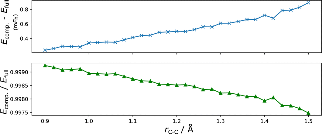
For the (8e,8o) CAS used for C2, the compression method discussed in Section 3.2 yields a total of 722 determinants in the compressed reference space. Here we show the results for the C2/cc-pVDZ system at separations of 0.9 to 1.5 Å. The performance of the compression scheme is shown in Fig. 5. Here we have employed the default quasi-Newton acceleration36 implemented in HANDE. We can see that despite the almost 7-fold reduction in the reference space (and consequently a similar reduction in computational cost), the errors are within chemical accuracy (1.6 mEh).
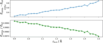 |
| | Fig. 5 The correlation energy for C2/cc-pVDZ at rC–C = 0.9–1.5 Å with the compressed set of 721 secondary references, relative to using the full CAS reference space. We observe that, despite a 7-fold reduction in the size of the reference space, the reductions in the correlation energy captured are much smaller, making this an attractive trade-off. The stochastic error bars are too small to be seen, due to the use of the semi-stochastic algorithm.25 | |
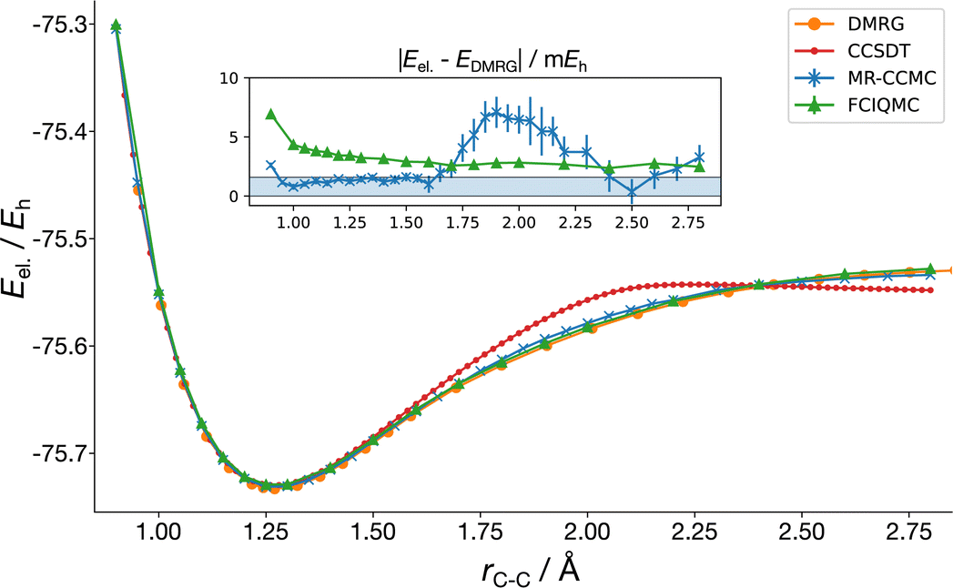
5.1.3 Binding curve of the carbon dimer.
Finally, we studied the X1Σ+g state of the carbon dimer in the cc-pVDZ basis using MR-CCMCSD with these accelerations. The carbon dimer is a challenging test case for electronic structure methods, and the challenge is two-fold: firstly, as mentioned in Section 4, the X1Σ+g state becomes very nearly degenerate with the exceptionally low-lying B1Δg state at stretched bond lengths,37 and both states descend to the Ag state in the commonly used D2h point-group symmetry, rendering it very challenging to distinguish both states without the use of the Lz symmetry, with one paper resorting to tracking individual CI coefficients;33 secondly, there is an abundance of avoided crossings, and specifically, the first excited B′1Σ+g state participates in an avoided crossing with the ground state at a bond length of around 1.6 Å,38 resulting in a change in the most highly weighted diabatic state (i.e., determinant). This makes MR-CCMC calculations based on RHF orbitals exhibit long-imaginary-time instabilities for stretched geometries, which preclude obtaining accurate estimators. The binding curve presented in Fig. 6 used the full (8e,8o) CAS as the reference space for a MR-CCMCSD calculation, with orbitals obtained using PySCF from an (8e,8o) state-average CASSCF calculation over the lowest three 1Ag states (in the D2h point group). The orbital coefficients are still tagged with their corresponding D∞h irreducible representations, enabling us to perform the Lz transformation. We ensured that the πu manifold was included in the reference determinant that generates the Hilbert space and secondary references.
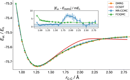 |
| | Fig. 6 The binding curve of the 1Σ+g state of C2/cc-pVDZ in the range of 0.9–2.8 Å separation. All-electron MR-CCMCSD calculations are based on CASSCF orbitals and use an (8e, 8o) CAS as a reference space, with clusters truncated at the double excitation level from this. The FCIQMC data is from ref. 39, and the DMRG data is from ref. 33, and the CCSDT data is from the ccpy package developed by Piecuch and coworkers.40 The inset shows the error in the MR-CCMC and FCIQMC energy relative to DMRG. | |
Non-parallelity errors (NPE), defined here as the difference between the maximal and minimal deviation from the DMRG energies, are shown in Table 2.
Table 2 The non-parallelity error, maximal and minimal absolute deviations of the carbon dimer binding curve calculated with MR-CCMCSD using an (8e,8o) CAS reference space, FCIQMC and CCSDT compared to the DMRG results. The numbers in parentheses indicate the bond length (in angstroms) at which the maximal/minimal absolute deviations occur
|
|
NPE/mEh |
Max AD/mEh |
Min AD/mEh |
| FCIQMC |
4.6 |
6.9 (0.9 Å) |
2.4 (2.4 Å) |
| MRCCMC |
10.4 |
7.1 (1.9 Å) |
0.4 (2.5 Å) |
| CCSDT |
45.5 |
28.1 (2.0 Å) |
0.3 (2.42 Å) |
5.2 Chebyshev propagator results
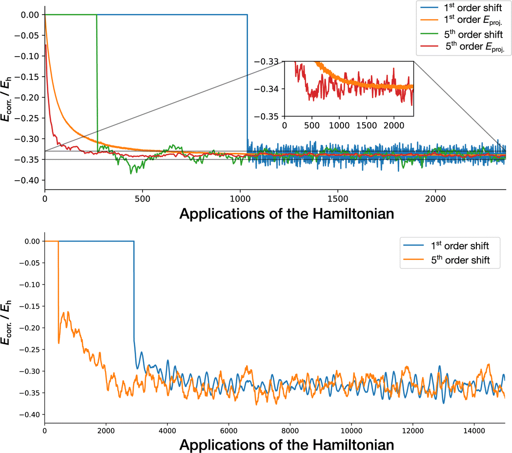
Fig. 7 shows an example of the power of the Chebyshev propagation, applied to MR-CCMCSD and i-FCIQMC calculations for C2. In MR-CCMCSD, the shoulder height is reached after around 50 iterations with the 5th-order wall-Chebyshev propagator, even with a higher target population than the corresponding 1st-order calculation. The dynamics is equilibrated essentially instantaneously, which means all that is left to do is collecting statistics. On an Intel(R) Xeon(R) E5-2650 v2 CPU, the calculation in the figure was run for only 2 hours on 6 physical cores. Without the Chebyshev projector, the same calculation takes around 24 hours with 12 physical cores to give the same statistical error bar.
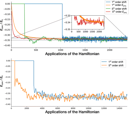 |
| | Fig. 7 QMC simulations of C2/cc-pVDZ at 1.2 Å separation, using the Chebyshev propagator. The top panel shows MR-CCMCSD calculations with a full (8e,8o) CAS reference space, run with the first- (simulated) and fifth-order Chebyshev projectors. The fifth-order calculation used a target population of 2 × 10⁶ and a shift damping parameter of 0.5, and the first-order calculations used a target population of 1 × 10⁶, and a shift damping parameter of 0.05. The inset shows that the projected energy only barely stabilises around the true value at the end of the calculation using the linear projector. The bottom panel shows i-FCIQMC calculations, run with the first- and fifth-order Chebyshev projectors. Both calculations used target populations of 2 × 10⁶ and a shift damping parameter of 0.5. The projected energy estimator for high-order wall-Chebyshev FCIQMC displays higher noise than the shift, so we do not show it here for clarity. All calculations were carried out with a two-stage harmonic forcing shift update scheme. | |
The same trend can be observed in the i-FCIQMC calculation. We note that, due to the formally large time step employed in wall-Chebyshev propagation, larger initiator thresholds are needed to easily stabilise calculations at low walker numbers than in conventional FCIQMC.
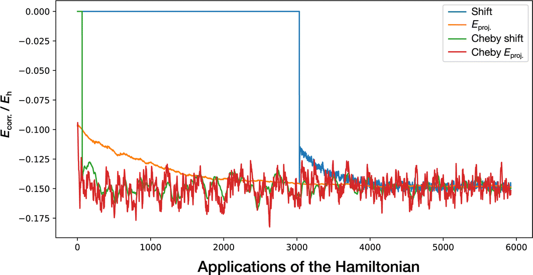
The following example shows Be2, a smaller, modestly multireference system, which, however, requires the inclusion of contributions beyond doubles from the HF reference to get a qualitatively correct binding curve. In Fig. 8, compared with the linear projector with a guessed δτ = 0.002, the second-order Chebyshev expansion shows a clear speed-up in convergence. In fact, the Chebyshev calculation took 66 applications of the Hamiltonian to reach the target population of 3 × 10⁶, whereas the linear projector took 3034 applications to reach the same target population.
 |
| | Fig. 8 The second-order projector (green and red lines) and the default linear projector (blue and orange lines) at δτ = 0.002 applied to MR-CCMCSD for the Be2/cc-pVQZ system at 2.5 Å separation, with a symmetry-screened (4e,8o) (full 2s, 2p valence) CAS as the reference space. Both calculations have a target population of 3 × 10⁶. | |
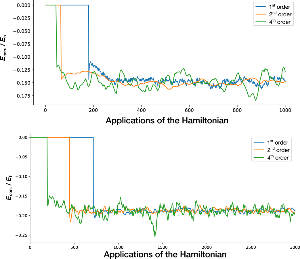
However, the second-order Chebyshev projector is expected to be as efficient as the linear projector with the maximum allowed time step (see Section 2.2). To provide a fairer comparison, we present in Fig. 9 the first-, second- and fourth-order Chebyshev projector applied to MR-CCMCSD and i-FCIQMC calculations for the Be2 system at 2.5 Å, in the cc-pVQZ and cc-pVTZ basis sets, respectively. The first-order Chebyshev projector is equivalent to a linear projector with δτ = 3/(EN−1 − E0), which is 2/3 of δτmax, but this maximal time step is commonly found to give rise to destabilising population blooms. Part of the benefit of our Chebyshev propagator algorithm is the automatic determination of the effective time steps, or ‘Chebyshev weights’, via the Gershgorin circle theorem, which in the first-order expansion limit reduces to an automatic way of choosing a good time step, instead of using trial and error.
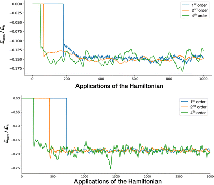 |
| | Fig. 9 The top panel shows an MR-CCMCSD propagation for Be2/cc-pVQZ at 2.5 Å separation with the (4e,8o) CAS reference space run with the first-, second- and fourth-order Chebyshev projectors. The bottom panel shows an i-FCIQMC propagation of Be2/cc-pVTZ at 2.5 Å separation, using the same propagators. Here we only show the shift as an estimator for Ecorr for clarity. | |
In Fig. 9 we can clearly see the reduction in time needed to reach the shoulder height. It is worth bearing in mind that for MR-CCMCSD the three calculations require different target populations to stabilise, with the first- and second-order projectors having target populations of 3 × 10⁶, and the fourth-order projector having a target population of 5 × 10⁶, which slightly increases the number of iterations required to reach the target population. In i-FCIQMC, despite using the smaller cc-pVTZ basis set, a target population of 5 × 10⁶ is used for all calculations.
Finally, as a demonstration of the applicability of the Chebyshev projector in different correlation regimes, we have computed the binding curve of the Be2/cc-pVTZ system using a (4e,8o) CAS as a reference space for MR-CCMCSD, using the fifth-order Chebyshev projector. CCSD(T) and semi-stochastic heat-bath configuration interaction with second-order perturbation correction (SHCI-PT2)41 results are also shown. The CCSD(T) results are from Psi4,28 and the SHCI-PT2 results are generated using the Dice plug-in to the PySCF package.29 For SHCI-PT2, the full (8e,28o) space was correlated, and hence it can be considered a surrogate for FCI results. The variational threshold was set to ε1 = 8 × 10⁻⁵Eh, and the PT2 threshold was set to ε2 = 1 × 10⁻⁸Eh, using Nd = 200 deterministic determinants, with 5 PT2 iterations. Fig. 10 shows the binding curves. The cc-pVTZ basis is known to severely overbind the beryllium dimer,42 compared to the experimental value of 934.9 ± 2.5 cm−1.43–45 Despite this, the MR-CCMC method using the Chebyshev projector was able to provide consistently better descriptions of the binding curve than the ‘gold-standard’ CCSD(T). The MR-CCMC results are close to, but not qualitatively the same as, FCI results near the equilibrium, where static correlation dominates,46 and are near-identical to FCI results in the stretched region, where dynamic correlation dominates, and a compact coupled-cluster representation of the wavefunction is beneficial.
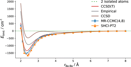 |
| | Fig. 10 The binding curves of the beryllium dimer using the cc-pVTZ basis, computed using the CCSD, CCSD(T), MR-CCMCSD with a (4e,8o) CAS, and SHCI-PT2 methods. The empirical binding curve from ref. 45 and 47 is also shown for comparison. | |
6 Conclusions
We presented here a series of algorithmic changes that can be used to accelerate the MR-CCMC algorithm in particular and QMC algorithms in general.
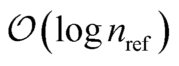
Specific to the MR-CCMC algorithm, we have introduced a BK-tree-based search algorithm to verify whether proposed clusters and spawns are within the accepted manifold for a given reference space. This reduces the scaling of this step from  to
to  , which translates to an 8× speed-up for the molecular systems studied. We have also designed a compression method for the reference space, which preserves only what we expect to be the most significant reference determinants. This decreases the size of the space by close to an order of magnitude. Finally, we have shown that only including references that belong to the same symmetry sector as the desired solution is also effective as a means to reduce the size of the reference space, while introducing only negligible additional error to the results.
We have also developed a new projector based on the Chebyshev polynomial expansion of the wall function, which significantly accelerates the convergence of QMC calculations. In an example calculation on the Be2 molecule, this reduced the number of Hamiltonian applications needed to reach the target population by two orders of magnitude. The wall-Chebyshev projector is generally applicable to different QMC algorithms, including FCIQMC and (MR-)CCMC approaches, so we believe that, together with many recent developments in increasing the apparent scarcity of the Hamiltonian and optimising the shift behaviour,21,48,49 it is a promising step in expanding the range of applications for these methods.
Author contributions
ZZ, MAF and AJWT all contributed to the conceptualization of the project. ZZ developed the necessary software and analysed the data, under supervision from MAF and AJWT. The manuscript was written by ZZ and MAF, with input from all authors.
Conflicts of interest
There are no conflicts to declare.
A Appendix
A.1 Higher-order Taylor series expansions of the exponential projector
In ref. 19 it was proposed that there is no gain in going to higher-order Taylor expansions of the exponential projector, because all orders of expansion have γ = τ (see Appendix A.3). The conclusion is correct, but for a more subtle reason that we will now explain. The mth-order Taylor series expansion of gexp is| |  | (29) |
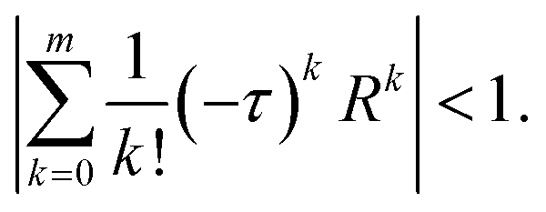
Eqn (6) in ref. 19 requires that g(EN−1) < 1, so, defining the spectral range R = EN−1 − E0, we have| | 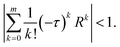 | (30) |
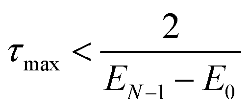
The m = 1 case leads to the familiar requirement in DMC, FCIQMC and CCMC that| | 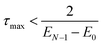 | (31) |
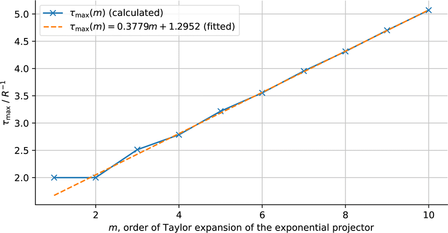
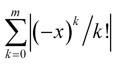
and solving eqn (30) numerically shows that higher-order expansions lead to larger maximum allowed τ. In fact, asymptotically, τmax increases linearly with a gradient of 1/e ≈ 0.368 (see Fig. 11). So, naïvely we can expect the efficiency to increase linearly with m. To prove the linearity, we note that τmaxR > 1, and we can approximate  (x ≡ τR) with the leading order term |(−x)m|/m!, and so we are left withwhere we used the Stirling’s formula in the second line.
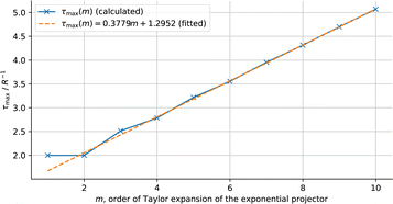 |
| | Fig. 11 Calculated and fitted τmax as a function of the order of Taylor expansion of the exponential projector. There is indeed no gain whatsoever in going to the second-order Taylor expansion, but there is in going to yet higher orders. | |
Therein lies the real reason for not using higher-order expansions: a naïve implementation requires m(m + 1)/2 applications of the Hamiltonian per projection, and even a factorised implementation would require m applications per projection, not to mention the lack of closed forms for the roots of the mth-order expansion, due to the Abel–Ruffini theorem,50 which shows that no analytical solution can exist for m ≥ 5. In any case, the overall efficiency stays constant at best. Therefore, the conclusion that no gains can be made is correct, although a more tortuous argument is needed.
A.2 Properties of the wall-Chebyshev projector
Assuming the entire spectral range is re-scaled such that x ∈ [−1,1], where x = 2(E − E0)/R − 1, and R = EN−1 − E0 is the spectral range or the Hamiltonian, the Chebyshev expansion coefficients of the wall function is| | 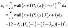 | (33) |
where the second line uses the fact that the wall function is zero everywhere but at the lower bound, so the weight function (1 − x2)−1/2 has the same action as the delta function centred at −1, δ(x + 1). The last equality exploits a well-known identity of the Chebyshev polynomials.51 We can then write the mth-order expansion as| | 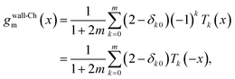 | (34) |
where the last equality exploits the fact that Tk has the same parity as k,51 and we scale the sum such that gwall-Chm(−1) = 1.
To obtain an analytical expression for the zeroes of the wall-Chebyshev projector, we use the trigonometric definition of the Chebyshev polynomials. Inverting the sign of the argument in eqn (34), we have
| | 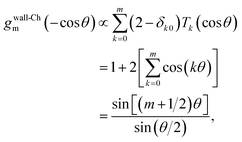 | (35) |
where the last equality is the Dirichlet kernel.
52 The zeroes of
gwall-Chm(
x) are then transparently
| | 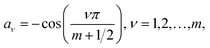 | (36) |
where the negative sign accounts for the sign inversion in
eqn (35). In an arbitrary spectral range other than [−1,1], these zeroes are
| |  | (37) |
Knowing its zeroes, we can decompose
gwall-Chm(
x) into a product of linear projectors:
| |  | (38) |
where the numerators ensure
gwall-Chm(
E0) = 1.
A.3 Convergence properties of projectors
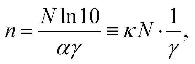
We summarise here some important properties of generators. The asymptotic rate of convergence of a propagator is dominated by the slowest-decaying eigencomponent:| | 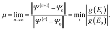 | (39) |
Zhang and Evangelista19 suggested that, in the common case that the first excited state is the slowest-decaying component, and that the first excited energy is small compared to the spectral range of Ĥ, the above can be approximated as| | | μ ≈ |1 + (E1 − E0)g′(E0)| ≡ |1 − αγ|, | (40) |
where γ = −g′(E0) is the convergence factor for g. We now derive the relation given in ref. 53 that γ is approximately the number of times, n, that g needs to be applied to achieve an error in the norm, ε = ‖Ψ(n) − Ψ0‖ to the Nth decimal place:| | | ε = 10−N ≈ (1 − αγ)n | (41a) |
| | 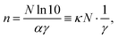 | (41c) |
where κ = ln10/(E1 − E0) is the convergence prefactor, which is inversely proportional to the first excited energy gap.
Acknowledgements
ZZ was in part funded by the U.S. Department of Energy under grant DE-SC0024532. MAF thanks Corpus Christi College, Cambridge and the Cambridge Trust for a studentship, as well as Peterhouse for funding through a Research Fellowship. This work used the ARCHER2 UK National Supercomputing Service (https://www.archer2.ac.uk).
Notes and references
- W. L. McMillan, Phys. Rev., 1965, 138, A442 CrossRef.
- D. Ceperley, G. V. Chester and M. H. Kalos, Phys. Rev. B: Solid State, 1977, 16, 3081 CrossRef CAS.
- J. B. Anderson, J. Chem. Phys., 1975, 63, 1499–1503 CrossRef CAS.
- J. B. Anderson, J. Chem. Phys., 1976, 65, 4121–4127 CrossRef CAS.
- J. B. Anderson, J. Chem. Phys., 1980, 73, 3897 CrossRef CAS.
- J. C. Grossman, J. Chem. Phys., 2002, 117, 1434–1440 CrossRef CAS.
- N. Nemec, M. D. Towler and R. J. Needs, J. Chem. Phys., 2010, 132, 034111 CrossRef PubMed.
- S. J. Cox, M. D. Towler, D. Alfè and A. Michaelides, J. Chem. Phys., 2014, 140, 174703 CrossRef PubMed.
- P. Ganesh, J. Kim, C. Park, M. Yoon, F. A. Reboredo and P. R. C. Kent, J. Chem. Theory Comput., 2014, 10, 5318–5323 CrossRef CAS PubMed.
- F. Della Pia, A. Zen, D. Alfè and A. Michaelides, J. Chem. Phys., 2022, 157, 134701 CrossRef CAS PubMed.
- G. H. Booth, A. J. W. Thom and A. Alavi, J. Chem. Phys., 2009, 131, 054106 CrossRef PubMed.
- A. J. W. Thom, Phys. Rev. Lett., 2010, 105, 263004 CrossRef PubMed.
- G. C. Wick, Phys. Rev., 1954, 96, 1124–1134 CrossRef CAS.
-
T. Helgaker, P. Jorgensen and J. Olsen, Molecular Electronic-Structure Theory, John Wiley & Sons, 2014 Search PubMed.
- J. S. Spencer and A. J. W. Thom, J. Chem. Phys., 2016, 144, 084108 CrossRef PubMed.
-
I. Shavitt and R. J. Bartlett, Many-Body Methods in Chemistry and Physics: MBPT and Coupled-Cluster Theory, Cambridge University Press, Cambridge, 2009 Search PubMed.
- M.-A. Filip, C. J. C. Scott and A. J. W. Thom, J. Chem. Theory Comput., 2019, 15, 6625–6635 CrossRef CAS PubMed.
- D. I. Lyakh, M. Musiał, V. F. Lotrich and R. J. Bartlett, Chem. Rev., 2012, 112, 182–243 CrossRef CAS PubMed.
- T. Zhang and F. A. Evangelista, J. Chem. Theory Comput., 2016, 12, 4326–4337 CrossRef CAS PubMed.
-
S. Geršgorin, Bulletin de l’Académie des Sciences de l’URSS. Classe des sciences mathématiques et na, 1931, pp. 749–754 Search PubMed.
- M. Yang, E. Pahl and J. Brand, J. Chem. Phys., 2020, 153, 174103 CrossRef CAS PubMed.
- W. A. Vigor, J. S. Spencer, M. J. Bearpark and A. J. W. Thom, J. Chem. Phys., 2016, 144, 094110 CrossRef CAS PubMed.
- R. W. Hamming, Bell Syst. Tech. J., 1950, 29, 147–160 CrossRef.
- W. A. Burkhard and R. M. Keller, Commun. ACM, 1973, 16, 230–236 CrossRef.
-
Z. Zhao, MPhil thesis, University of Cambridge, Cambridge, UK, 2022 Search PubMed.
- D. Cleland, G. H. Booth and A. Alavi, J. Chem. Phys., 2010, 132, 041103 CrossRef PubMed.
- T. H. Dunning, J. Chem. Phys., 1989, 90, 1007–1023 CrossRef CAS.
- D. G. A. Smith, L. A. Burns, A. C. Simmonett, R. M. Parrish, M. C. Schieber, R. Galvelis, P. Kraus, H. Kruse, R. Di Remigio, A. Alenaizan, A. M. James, S. Lehtola, J. P. Misiewicz, M. Scheurer, R. A. Shaw, J. B. Schriber, Y. Xie, Z. L. Glick, D.
A. Sirianni, J. S. O’Brien, J. M. Waldrop, A. Kumar, E. G. Hohenstein, B. P. Pritchard, B. R. Brooks, H. F. Schaefer, A. Y. Sokolov, K. Patkowski, A. E. DePrince, U. Bozkaya, R. A. King, F. A. Evangelista, J. M. Turney, T. D. Crawford and C. D. Sherrill, J. Chem. Phys., 2020, 152, 184108 CrossRef CAS PubMed.
- Q. Sun, T. C. Berkelbach, N. S. Blunt, G. H. Booth, S. Guo, Z. Li, J. Liu, J. D. McClain, E. R. Sayfutyarova, S. Sharma, S. Wouters and G. K.-L. Chan, WIREs Comput. Mol. Sci., 2018, 8, e1340 CrossRef.
- K. Guther, R. J. Anderson, N. S. Blunt, N. A. Bogdanov, D. Cleland, N. Dattani, W. Dobrautz, K. Ghanem, P. Jeszenszki, N. Liebermann, G. L. Manni, A. Y. Lozovoi, H. Luo, D. Ma, F. Merz, C. Overy, M. Rampp, P. K. Samanta, L. R. Schwarz, J. J. Shepherd, S. D. Smart, E. Vitale, O. Weser, G. H. Booth and A. Alavi, J. Chem. Phys., 2020, 153, 034107 CrossRef CAS PubMed.
- A. A. Holmes, H. J. Changlani and C. J. Umrigar, J. Chem. Theory Comput., 2016, 12, 1561–1571 CrossRef CAS PubMed.
- G. H. Booth, S. D. Smart and A. Alavi, Mol. Phys., 2014, 112, 1855–1869 CrossRef CAS.
- S. Wouters, W. Poelmans, P. W. Ayers and D. Van Neck, Comput. Phys. Commun., 2014, 185, 1501–1514 CrossRef CAS.
- S. Sharma, J. Chem. Phys., 2015, 142, 024107 CrossRef PubMed.
- J. S. Spencer, N. S. Blunt, S. Choi, J. Etrych, M.-A. Filip, W. M. C. Foulkes, R. S. T. Franklin, W. J. Handley, F. D. Malone, V. A. Neufeld, R. Di Remigio, T. W. Rogers, C. J. C. Scott, J. J. Shepherd, W. A. Vigor, J. Weston, R. Xu and A. J. W. Thom, J. Chem. Theory Comput., 2019, 15, 1728–1742 CrossRef CAS PubMed.
- V. A. Neufeld and A. J. W. Thom, J. Chem. Theory Comput., 2020, 16, 1503–1510 CrossRef CAS PubMed.
- M. L. Abrams and C. D. Sherrill, J. Chem. Phys., 2004, 121, 9211–9219 CrossRef CAS PubMed.
- A. J. C. Varandas, J. Chem. Phys., 2008, 129, 234103 CrossRef CAS PubMed.
- G. H. Booth, D. Cleland, A. J. W. Thom and A. Alavi, J. Chem. Phys., 2011, 135, 084104 CrossRef PubMed.
-
K. Gururangan, J. E. Deustua and P. Piecuch, CCpy: A coupled-cluster package written in Python, https://github.com/piecuch-group/ccpy.
- S. Sharma, A. A. Holmes, G. Jeanmairet, A. Alavi and C. J. Umrigar, J. Chem. Theory Comput., 2017, 13, 1595–1604 CrossRef CAS PubMed.
- K. Guther, A. J. Cohen, H. Luo and A. Alavi, J. Chem. Phys., 2021, 155, 011102 CrossRef CAS PubMed.
- J. M. Merritt, V. E. Bondybey and M. C. Heaven, Science, 2009, 324, 1548–1551 CrossRef CAS PubMed.
- V. V. Meshkov, A. V. Stolyarov, M. C. Heaven, C. Haugen and R. J. LeRoy, J. Chem. Phys., 2014, 140, 064315 CrossRef PubMed.
- K. Patkowski, V. Špirko and K. Szalewicz, Science, 2009, 326, 1382–1384 CrossRef CAS PubMed.
- M. El Khatib, G. L. Bendazzoli, S. Evangelisti, W. Helal, T. Leininger, L. Tenti and C. Angeli, J. Phys. Chem. A, 2014, 118, 6664–6673 CrossRef CAS PubMed.
- X. W. Sheng, X. Y. Kuang, P. Li and K. T. Tang, Phys. Rev. A: At., Mol., Opt. Phys., 2013, 88, 022517 CrossRef.
- K. Ghanem, A. Y. Lozovoi and A. Alavi, J. Chem. Phys., 2019, 151, 224108 CrossRef PubMed.
- K. Ghanem, K. Guther and A. Alavi, J. Chem. Phys., 2020, 153, 224115 CrossRef CAS PubMed.
- R. G. Ayoub, Arch. Hist. Exact Sci., 1980, 23, 253–277 CrossRef.
-
K. F. Riley, M. P. Hobson and S. J. Bence, Mathematical Methods for Physics and Engineering: A Comprehensive Guide, Cambridge University Press, 3rd edn, 2006 Search PubMed.
- P. G. L. Dirichlet, J. Reine Angew. Math., 1829, 4, 157–169 Search PubMed.
- R. Kosloff and H. Tal-Ezer, Chem. Phys. Lett., 1986, 127, 223–230 CrossRef CAS.
Footnotes |
| † Present address: Department of Chemistry, Emory University, Atlanta, GA, USA. |
| ‡ Present address: Max Planck Institute for Solid State Research, Stuttgart, Germany. |
|
| This journal is © The Royal Society of Chemistry 2024 |
Click here to see how this site uses Cookies. View our privacy policy here.  Open Access Article
 This Open Access Article is licensed under a
  *,
Maria-Andreea
Filip‡
*,
Maria-Andreea
Filip‡
 , to the time-dependent Schrödinger’s equation
 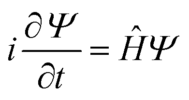 , one obtains the imaginary time Schrödinger’s equation:
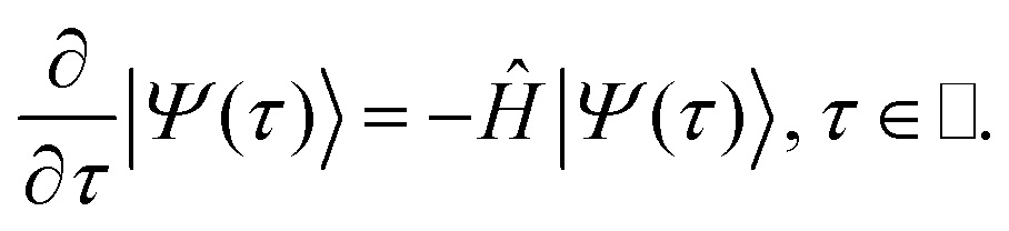

 . We can see that, if S = E0, in the limit of τ → ∞, we obtain the ground state of the full Hamiltonian.
 :
:
 contributions on both sides to write
 clusters are formed randomly by combining present excitors according to specific biasing rules.15


 operation, where nref is the number of secondary references. The subroutine that decides whether a spawn is accepted is the second most frequently called subroutine in the program, after the excitation generator. Therefore, a linear search in this step can quickly become prohibitively expensive in a moderate to large reference space (nref > 1000, for example). We note that traditional data structures and search algorithms, such as a binary search on a sorted list of secondary references, would not work here, as the definition of ‘distance’ in this case, i.e., excitation-rank, is non-Euclidean. A search algorithm in a general metric space is therefore needed.
 time using a recursive tree traversal algorithm. The tree construction and search algorithms are pictured in Fig. 4.
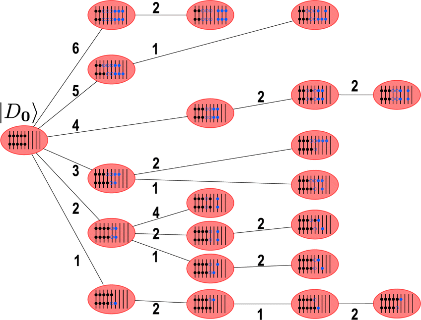

 to
to  , which translates to an 8× speed-up for the molecular systems studied. We have also designed a compression method for the reference space, which preserves only what we expect to be the most significant reference determinants. This decreases the size of the space by close to an order of magnitude. Finally, we have shown that only including references that belong to the same symmetry sector as the desired solution is also effective as a means to reduce the size of the reference space, while introducing only negligible additional error to the results.
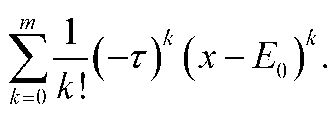
 (x ≡ τR) with the leading order term |(−x)m|/m!, and so we are left with