Enhancing molecular safety and health assessment via index smoothing and prioritisation
Received
14th August 2017
, Accepted 17th October 2017
First published on 17th October 2017
Abstract
In recent decades, safety and health aspects have received much attention in the field of computer-aided molecular design (CAMD). To satisfy the more stringent requirements of regulating agencies, a product must not only achieve its desired function as defined by the customers but also meet safety and health criteria to ensure that the risk posed to users can be minimised to acceptable levels. One of the promising methods to efficiently measure the safety and health aspects of chemical substances is the application of inherent safety and occupational health indexes. These indexes consist of multiple safety and health hazard parameters to assess the physicochemical properties of molecules. The properties are divided into multiple sub-ranges, each of which is assigned a penalty value that corresponds to its degree of hazard. In this work, the penalty values are computed to ensure a smooth transition from one category to another. The quantification of the overall safety and health performance is improved by combining the ordered weighted averaging (OWA) operator method with the analytic hierarchy process (AHP). A case study on solvent design for carotenoid extraction from palm pressed fibre (PPF) illustrates the proposed methodology.
Design, System, Application
The proposed CAMD framework aims to generate molecules that are optimised with respect to property functionalities and the aspects of safety and health. The molecular functionalities are defined by specifying a set of target properties to ensure that the generated molecules are able to demonstrate the desired performance and characteristics. Meanwhile, the safety and health attributes of the molecules are evaluated by inherent safety and health indexes, which utilise a scoring scheme to reflect on the inherent hazard level of the molecules. The main highlight of this work is to enhance the scoring scheme of the indexes and improve the approach to quantify the overall hazard level displayed by a molecule. Structural constraints are introduced to ensure that only feasible molecules with no free bonds can be generated. An optimisation technique known as the fuzzy optimisation formulation is employed to simultaneously optimise the target properties and the overall safety and health index score. This methodology is capable of serving as a screening tool for any molecular design problem to synthesise molecules with high property functionality performance and at the same time exhibit favourable safety and health characteristics.
|
1. Introduction
In chemical process design and development, the selection of chemicals has a crucial impact on plant safety and occupational health. In cases where hazardous chemicals are utilised in a process, the most common approach to handle such risks is to install an add-on layer of protection (LOP) via technological safety barriers. However, several past accidents such as the Flixborough (1974) and Piper Alpha (1987) disasters have occurred due to the failure of the LOP in controlling hazards. This is because safety barriers do not actually eliminate hazards.1 Instead of merely mitigating the hazards, the best way is to handle these safety and health concerns by eliminating them at their sources.2 Thus, one important approach to this problem is to replace hazardous chemicals with less harmful ones.
The use of chemicals with intrinsically reduced risks is one of the basic principles of inherent safety design (ISD), which was proposed by Kletz3 to eliminate or minimise hazards present in the plant. The fundamental aim of ISD is to avoid the use of hazardous substances, minimise the inventories of such substances, and consider simpler processes with milder process conditions.4 Many research works have been conducted to evaluate inherent safety in the process plant, mainly the selection of a chemical process route during the early design stage. Edwards and Lawrence5 were the first to develop the Prototype Index for Inherent Safety (PIIS) by using several safety parameters to measure the safety level of different process routes in the conceptual design stage. These parameters (or sub-indexes) were then formulated into an index scoring scheme to quantify the hazard level of the process routes. Following this first attempt, Heikkilä6 extended the PIIS by introducing the Inherent Safety Index (ISI) to also assess the inherent safety in process route selection, but during the preliminary design phase. A wider range of safety sub-indexes was considered in ISI.
Meanwhile, the goal of inherent occupational health is derived from inherent safety, which is mainly to reduce occupational health risks to workers in the workplace environment. Hassim and Edwards7 presented the Process Route Healthiness Index (PRHI) for the assessment of occupational health hazards posed by alternative chemical process routes. Hassim and Hurme8 then developed the Inherent Occupational Health Index (IOHI) for the evaluation of occupational health hazards by focusing on process conditions and health properties of chemicals during the R&D phase. Likewise, IOHI employs several health sub-indexes to measure the health risk level through the allocation of penalty scores to the alternative process routes.
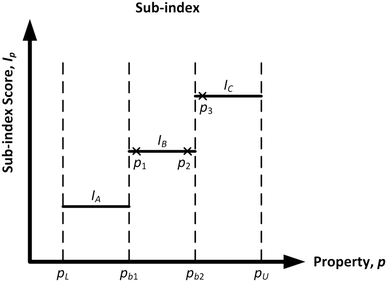
To adopt the concept of inherent safety and occupational health, the hazardous chemicals used in a process route have to be replaced with less harmful ones. The computer-aided molecular design (CAMD) technique has been adequately employed for the exploration of molecular structures with minimised risk that are also best suited for a particular chemical process.9 The two main design criteria in the CAMD framework are product functionalities and its inherent safety and health level. Chemical-related sub-indexes from the inherent safety and health indexes are adopted to assist in the design of an inherently safer and healthier molecule. For each sub-index, the physical and chemical properties of molecules are used to measure the potential hazards. The properties in these sub-indexes are divided into multiple sub-ranges, and numerical penalty scores are then assigned to the sub-ranges. The general profile for the assignment of sub-index scores is shown in Fig. 1.
 |
| | Fig. 1 General trend for sub-index score allocation. | |
As shown in Fig. 1, pL and pU are the lower and upper bounds of the feasible property range, respectively. There are two property boundary values in the graph, namely pb1 and pb2, which are the points where the scores change from one value to another. This score allocation method has two weaknesses. First, property values that fall in the same sub-range are deemed to possess a similar hazard level. For instance, using the example in Fig. 1, there are three different molecules with property values of p1, p2 and p3 plotted in the graph. Both p1 and p2 fall in the sub-range of “pb1 to pb2.” These two property values are considered to have the same hazard level, as they share a similar sub-index score of IB. However, as p1 is located near the lower edge of the sub-range while p2 is almost at the other edge of the sub-range, they should not be considered to exhibit the same level of hazard. Secondly, the other main limitation of this current score allocation method is the discontinuity at the boundary values, which may distort the comparison of alternatives that are near these limits. This discontinuity may create an artificial distinction between otherwise similar molecules that belong to adjacent categories near a sharp boundary. This issue may affect the reliability of CAMD in generating a molecule with minimised safety and health risk. The two molecules with property values of p2 and p3 as shown in Fig. 1 are used to illustrate this limitation. Both p2 and p3 are located considerably nearer to each other as compared to the distance between p1 and p2. However, the former pair possesses different sub-index scores as they are separated by a sharp boundary where the score changes abruptly. As a result, p2 and p3 fall in two adjacent sub-ranges even though they have a relatively small difference in property value. Hence, there is a need to revise the scores at the edges of the sub-range to enhance the representation of the molecular hazard level.
In addition, the current method of quantifying the inherent risk level of a molecule is by summing up all the sub-index scores from the selected safety and health sub-indexes. Since the aim of CAMD is to find a suitable molecular candidate with reduced hazard, one of the design objectives is to minimise the summation of all sub-index values for reduced hazards.9 However, a molecule with the lowest total index score may not necessarily display a low risk level with respect to all sub-indexes. This is because one of its sub-indexes may exhibit a very high score, while the remaining sub-indexes have relatively lower scores to compensate for the high-scoring sub-index. In reality, any molecule demonstrating a highly hazardous attribute with respect to a specific sub-index (e.g. highly toxic) is usually deemed a dangerous chemical, and that particular molecule is therefore screened out in the chemical selection phase. In addition, this summation of scores method presumes that all sub-indexes have equal impact on the plant safety and occupational health of the workers. Hence, there is a need to address this limitation on hazard quantification so that the more hazardous or greater impact sub-index will be penalised to a greater extent.
In this paper, the two weaknesses resulting from the current index scoring scheme will be addressed by smoothing the scorings near the boundary values. This eliminates the allocation of similar scores within a particular sub-range and removes the sharp property boundaries. This modification of index scoring is able to enhance the comparison of molecular hazard levels in CAMD. As for the limitation on hazard quantification, a weight factor will be allocated to each sub-index when determining the overall risk level of the molecules. This ensures that the severity of each sub-index is taken into account when the CAMD programming is searching for a low-risk molecule. However, one challenge here is to identify a systematic technique to decide on the appropriate values for the weight factors. This paper will explore the utilisation of the analytic hierarchy process (AHP), which is a structured multi-attribute decision analysis approach, to determine a set of suitable weights assigned to the sub-indexes.
To summarise, this work will improve the CAMD framework with the integration of safety and health aspects developed by Ten et al.9 The two improvements made are the smoothing of sub-index scorings at their respective property boundary values and the allocation of weight factors to each sub-index to distinguish the impact level of different sub-indexes. The structure of this paper is organised as follows. Section 2 presents the background and methodology of the CAMD approach. The consideration of safety and health aspects into CAMD by different works is also discussed. Section 3 details the concept and mathematical algorithm of AHP. Section 4 illustrates the methodology of this work which combines AHP with the ordered weighting operator (OWA) for determining the weighting factor for each sub-index as shown in section 4.3. The OWA approach enables conditional weighting (i.e., a priority can be calibrated based on the weaker features of any given alternative, thus resulting in a more conservative solution). The smoothing of sub-index scores is depicted in section 4.5. Section 5 presents the application of the proposed methodology in a case study, which is to identify the best solvent to extract carotenoids found in the residual oil in palm pressed fibre (PPF).
2. Computer-aided molecular design (CAMD)
Over the years, the concept of safety, health and environment criteria has received much attention in the increasingly demanding global business environment. One way to attain sustainable development in the chemical industries is the discovery and development of new chemicals such as industrial solvents, refrigerants, and drugs to increase the process efficiency while also minimising the potential adverse impacts on safety, health and the environment. In these days, the exploration of new chemicals can be carried out using the CAMD technique, which is deemed to be an efficient tool for the rapid search of a molecule or molecular structure from a given set of molecule building blocks that matches the desirable target properties.10 In order to estimate the target properties of molecules, most CAMD methods have relied on group contribution based property prediction methods. The general form of a group contribution method (GCM) model developed by Marrero and Gani11 is given by the following equation:| |  | (1) |
where Ci is the contribution of the first-order group of type i with Ni occurrences, Dj the contribution of the second-order group of type j with Mj occurrences and Ek the contribution of the third-order group of type k with Ok occurrences. The left-hand side of eqn (1) is a function f(P) to estimate property P, which is distinct for each property P.
For the past two decades, numerous works on CAMD have considered the aspects of safety, health and environment when designing chemicals. Some earlier works have considered the replacement of chlorofluorocarbons (CFCs) as refrigerants with less harmful substitutes, since the use of CFCs has resulted in the depletion of the ozone layer. Duvedi and Achenie12 presented a mixed integer nonlinear programming (MINLP) approach in the search for alternative safe refrigerants to replace Freon 12. Karunanithi et al.13 imposed safety property constraints to develop solvents for solution crystallisation. Papadokonstantakis et al.14 considered several design factors such as thermodynamic performance, environmental impact, hazard evaluation, and economic analysis with predictive molecular-based approaches, CAMD, and process modelling for the synthesis of a solvent-based post-combustion CO2 capture system. Palma-Flores et al.15 adopted safety and health parameters for the working fluid design of a low-temperature waste heat recovery with the organic Rankine cycle (ORC). Gerbaud et al.16 introduced health, safety and security requirements for the substitution of aprotic highly dipolar solvents with itaconic acid derivatives. In most of these CAMD problems, the safety, health and environmental properties are implemented as constraints or limits, where molecules that do not satisfy the constraints are excluded. However, Lampe et al.17 stated that a trade-off between the performance of the excluded molecules and the investment cost for the installation of safety barriers should be assessed. Thus, simultaneous optimisation of product performance and their safety and health attributes as presented by Ten et al.9 is considered in this paper for synthesising molecules that meet both criteria.
3. Analytic hierarchy process (AHP)
As mentioned in section 1, the AHP method is applied for the allocation of weight factors to all safety and health sub-indexes. The AHP is described by Saaty18 as a theory of relative measurement that is now widely used for many decision-making problems. The application of AHP has three main principles, namely, problem decomposition, comparative judgements and synthesis of priorities. The stage of decomposition begins by breaking down a problem into smaller elements and structuring them into a hierarchy with different levels, where each level contains a finite number of elements. The top of the hierarchy is usually the objectives of the decision-making problem, the intermediate levels are represented by several criteria on which the subsequent levels depend, while the lowest level contains a list of potential alternatives. Each element in the hierarchy will serve as the criterion for all elements of the level below.19
In the stage of comparative judgements, pairwise comparisons of the relative strength or importance of n elements in the same hierarchy level are carried out with respect to a common aspect in the level above. The decision maker can compare any two elements (e.g. Ei and Ej) and assign a numerical scale aij as the ratio of their relative importance (i.e., wi/wj). If two elements being compared have equal importance, then aij would be given a value of one. If element Ei is considered to have higher importance than Ej, then aij would be greater than one. Once n(n − 1)/2 pairwise comparisons are completed among all elements, a positive reciprocal square matrix containing the comparative judgments is obtained as shown in eqn (2).
| |  | (2) |
In the comparison matrix, the reciprocal property aji = 1/aij (where aij > 0) always holds true for j = 1, 2, …, n and i = 1, 2, …, n, in which n represents the number of elements in the level. A measurement scale of 1 to 9 as shown in Table 1 is used to assign the numerical value to each aij.20 For instance, if element Ei is deemed to be strongly more important than Ej, then its aij value would be 5. Its corresponding reciprocal, aji, will then be equivalent to 1/5.
Table 1 The fundamental AHP scale20
| Numerical scale |
Definition (explanation) |
| 1 |
Equal importance (two elements contribute equally to the objective) |
| 3 |
Moderate importance of one over another (experience and judgement slightly favour one element over another) |
| 5 |
Essential or strong importance (experience and judgement strongly favour one element over another) |
| 7 |
Very strong importance (an element is strongly favoured and its dominance demonstrated in practice) |
| 9 |
Extreme importance (an element is strongly more favoured over another with the highest possible order of affirmation) |
| 2, 4, 6 and 8 |
Intermediate values between the two adjacent judgements (the judgement falls between two levels) |
| Reciprocals |
If element i has one of the above numbers allocated to it when compared with element j, then j has the reciprocal value when compared with i |
The relative strength or importance of all elements being compared has to be identified from the comparison matrix. To do this, a vector of ratio-scale priorities or weights, w, has to be computed from the matrix. First, in order to determine vector w, Saaty21 has suggested the principal eigenvalue method as shown in eqn (3):
where
A is the pairwise comparison matrix and
λmax is the maximum eigenvalue of matrix
A. The solution for vector
w is determined numerically by raising the matrix
A to a sufficiently large power, then summing over the rows and normalising them to obtain the weight vector
w = (
w1,
w2, …,
wn)
T. The summation of the weights in vector
w is equivalent to one. The value of
λmax can then be identified through
eqn (3). The next step is to determine the consistency of the comparison matrix. A matrix is considered to be perfectly consistent when its elements fulfil the following condition:
Given a problem with three elements where element Ei is considered to be more important than Ej, and Ej is more important than Ek. The problem is deemed to be inconsistent if element Ek has higher importance than Ei. Saaty21 has introduced eqn (5) and (6) to measure the extent of the deviation from consistency of the comparison matrix:
| |  | (5) |
| |  | (6) |
where CR is the consistency ratio, CI is the consistency index, and RI is a random consistency index that can be referred to Saaty.
21 The value of CR should be less than 0.1 or 10% for the deviation from consistency to be acceptable. If the calculated CR does not fall within this range, decision makers are asked to revise their comparative judgements. Since the AHP numerical scale as shown in
Table 1 ranges from one to nine, it is suggested that one should not consider more than seven elements for pairwise comparison in order to ensure the validity of numerical comparisons. In case of a problem with a large number of elements, hierarchical decomposition should be carried out by grouping the elements into comparability classes of approximately seven elements each.
19
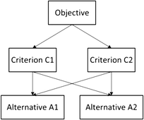
In the synthesis of priorities stage, the priorities are determined for each level beginning from the second level to the bottom level. Given an example decision-making problem which contains three levels is shown in Fig. 2. The top level is represented by the objective. In its second level, there are two criteria known as C1 and C2, in which the local priorities calculated by pairwise comparison with respect to the objective are 0.667 and 0.333, respectively. Meanwhile in the third level, each criterion is provided with two alternatives known as A1 and A2. If the local priorities of A1 and A2 with respect to criterion C1 were 0.75 and 0.25, respectively, while the local priorities of A1 and A2 with respect to C2 were 0.2 and 0.8, respectively; then the global priorities for A1 and A2 are synthesised by multiplying the local priorities by the priority of their respective criterion in the level above and then adding them for each element in a level according to the criteria it affects.19 Thus, the global priority for A1 can be calculated by (0.667 × 0.75) + (0.333 × 0.2) = 0.567, while the global priority for A2 is determined by (0.667 × 0.25) + (0.333 × 0.8) = 0.433. Alternative A1 is chosen as the preferred solution as it has a larger global priority than A2. In this work, the application of AHP to determine the weight factors is further illustrated in section 4.3.
 |
| | Fig. 2 Hierarchy for an example decision-making problem. | |
4. Methodology
4.1 Design objective and problem formulation
In this first stage, the design goal of a chemical product design problem is specified. In order to achieve the goal, suitable target properties are identified to ensure that the final synthesised product can function and behave in the desired manner. In most molecular design problems, the target properties are expressed by the physicochemical properties of the molecule. The target property will be selected either as an objective function to be optimised or as a property constraint to be fulfilled. A property range is introduced into each target property as shown in eqn (7) to ensure that the product can function optimally:where p represents target property, Vp denotes target property value, while vLp and vUp are the lower and upper bounds of the range, respectively.
4.2 Safety and health assessment
In this stage, the evaluation tool to measure the safety and health characteristics of the molecule is determined. As mentioned in section 1, all inherent safety and health indexes are developed by identifying parameters that have a significant contribution to the arising of adverse safety and health impacts. In this section, the parameters are adopted to measure the safety and health performance of the molecule. For the safety aspect, some of the prominent inherent indexes are the PIIS,5 ISI,6 and i-Safe.22 Meanwhile for the health aspect, the two established inherent indexes for the early design stage are the PRHI7 and IOHI.8 Each safety or health parameter is listed as a sub-index, in which a sub-index value will be allocated depending on the degree of potential hazard. A higher sub-index value indicates that the molecule exhibits a higher intrinsic hazard for that particular sub-index. The sub-indexes are mainly assessed by using the physicochemical properties of molecules. For example, the volatility sub-index from the IOHI as shown in Table 2 is evaluated by using the boiling point of a molecule. The boiling point can be estimated through the application property prediction method. The allocation of sub-index value depends on the input value of boiling point. This type of numerical assessment can be integrated into the mathematical-based CAMD optimisation model.
Table 2 Volatility (IV) sub-index8
| Factor |
Scoring detail |
Sub-index value |
| Volatility, IV |
Liquid and gas |
|
| Very low volatility (Tb > 150 °C) |
0 |
| Low (150 °C ≥ Tb > 50 °C) |
1 |
| Medium (50 °C ≥ Tb > 0 °C) |
2 |
| High (Tb ≤ 0 °C) |
3 |
The selected safety and health sub-indexes along with their corresponding properties being assessed are summarised in Table 3. The sub-index of toxicity is not chosen as one of the safety sub-indexes since it is evaluated by the sub-index of exposure limit in the health aspect. The sub-index scores for the two safety sub-indexes are taken from the NFPA flammability rating and ISI. Meanwhile, the sub-index scores for the five chosen health sub-indexes are taken from the PRHI, IOHI and NFPA health hazard rating.
Table 3 The selected safety and health sub-indexes with their properties
| Sub-index |
Property being assessed |
| Safety |
|
| Flammability, IFL |
Flash point (Fp) and boiling point (Tb) |
| Explosiveness, IEX |
Upper and lower explosion limits (UEL and LEL) |
| Health |
|
| Viscosity, Iη |
Viscosity (η) |
| Material phase, IMS |
Boiling point (Tb) and melting point (Tm) |
| Volatility, IV |
Boiling point (Tb) |
| Exposure limit, IEL |
Permissible exposure limit (PEL) |
| Acute health hazard, IAH |
LD50 for acute oral toxicity |
4.3 Determination of total weighted index score
Once all the relevant sub-indexes are identified (see section 4.2), the intrinsic hazard level of a molecule will then be quantified. A total index score, ISHI, is given to the molecule to depict the degree of its hazard. As shown by Ten et al.,9 the total index score assigned to a molecule is equivalent to the summation of all seven sub-index scores. A lower total index score is favourable as the molecule exhibits a lower magnitude of hazard. This method of measuring hazard treats all sub-indexes with equal importance, as they all have a similar weight of contribution towards the final total score. Assume that there are two molecules (M1 and M2) with their sub-index scores displayed in Table 4.
Table 4 The two molecules with their sub-index scores
| Molecule |
I
FL
|
I
EX
|
Iη
|
I
MS
|
I
V
|
I
EL
|
I
AH
|
I
SHI
|
| M1 |
1 |
1 |
2 |
1 |
0 |
4 |
1 |
10 |
| M2 |
2 |
2 |
2 |
1 |
1 |
2 |
1 |
11 |
From Table 4, it is shown that molecule M1 has a lower hazard than M2 as it has a lower ISHI value. However, the summation of all sub-index values to calculate ISHI does not really illustrate the molecular performance in each individual sub-index. Among the sub-indexes, IFL, IEX, IEL and IAH have the most severe penalty score of four, while Iη, IMS and IV have the most severe penalty score of three. The variation in score domain among each sub-index reflects the importance and impacts of the particular sub-index to the plant safety and occupational health. In Table 4, molecule M1 has an extremely high penalty score for IEL, which is also the most severe score for this sub-index. Therefore, molecule M1 is deemed to be extremely toxic. However, it still receives a lower ISHI score as its high IEL score is being ‘compensated for’ by the remaining six low-scoring sub-indexes. Even though molecule M2 has a higher ISHI value, all its seven sub-index values can be considered as moderately low. Such compensation cannot be justified since in many conventional molecular design problems, a molecule which is highly hazardous in any safety and health parameter is often screened out during the decision-making process.
In order to address this problem, a weighting factor can be introduced to each sub-index value in which a higher sub-index score (higher adverse impact to the plant) will be assigned with a larger weight. This can ensure that a higher-scoring sub-index will have a greater contribution to the final weighted ISHI value. This results in an inherently conservative weighing procedure, which can be managed by applying aggregation operators that have been developed to assist in aggregating information. Some of these methods include the max and min operators, arithmetic averaging (AA) operator, weighted AA (WAA) operator, geometric averaging (GA) operator, ordered weighted averaging (OWA) operator, etc.23 In this work, the weights are assigned conditionally based on the ordered position of the sub-index scores. The allocation of weight in this manner can be adequately done with the application of the OWA operator method introduced by Yager.24 An OWA operator of dimension n is a function
with an associated
n vector
where
Besides,
| |  | (8) |
where
bj is the
jth largest of the
ai. The principal characteristic of the OWA operator is the reordering step, in which an argument
ai is not associated with a specific weight
wi, but a weight
wi is associated with a specific rank
i of the arguments.
24 Thus, the weights determined
via AHP can be assigned conditionally to the criteria based on the logic that there should be more weight placed on the weaker and more critical features of a given alternative. This approach can thus yield a more conservative approach than simply assigning fixed weights to the criteria. For the measurement of safety and health aspects of the molecules, a sub-index with a weaker performance (or a more severe score) is assigned a higher weight to penalise the high hazard condition as demonstrated by the molecules. The quantification of the overall hazard exhibited by the molecules can be done using
eqn (8), where the right-hand side is the summation of all multiplication between the sub-index values and their corresponding weights. Among the seven sub-indexes, the one with the largest penalty score is multiplied by the largest weight, while the sub-index with the second largest penalty score will be multiplied by the second largest weight and so on. The function on the left-hand side is the total weighted index score,
ISHI,w. In order to determine the seven weight factors, a systematic technique known as analytic hierarchy process (AHP) can be utilised. Previously, Yager and Kelman
25 have come out with an extension of AHP using the OWA operator, which integrates linguistic quantifiers of the OWA operator to enhance decision making considered in the AHP. Lamata
26 ranked the alternatives in multiattribute decision making using fuzzy AHP with OWA operators. Boroushaki and Malczewski
27 proposed the incorporation of a geographic information system (GIS) and the extension of AHP using the quantifier-guided OWA procedure.
The purpose of AHP in this work is to determine the weights introduced to the sub-indexes, which represent the impact or contribution of the specific sub-index to ISHI,w. In the first stage of AHP, the problem is presented in the form of a hierarchy that contains several elements. The hierarchy for this weight determination problem is shown in Fig. 3.
 |
| | Fig. 3 Hierarchy for the weight determination of sub-indexes. | |
In Fig. 3, the topmost level is the goal of this AHP problem, which is to determine the weight of the sub-indexes. The sub-index with the highest scoring is named “rank 1 sub-index” or SIR1, the second highest scoring sub-index is defined as “rank 2 sub-index” or SIR2 and so on. The seven sub-indexes are the elements which contribute to the final ISHI,w value. In the next step, pairwise comparisons are considered among all seven sub-indexes to assess the relative importance and impact towards the final weighted index score. The complete pairwise comparison matrix is shown in Table 5.
Table 5 Pairwise comparison matrix
|
|
SIR1 |
SIR2 |
SIR3 |
SIR4 |
SIR5 |
SIR6 |
SIR7 |
| SIR1 |
1 |
2 |
3 |
4 |
5 |
6 |
7 |
| SIR2 |
1/2 |
1 |
2 |
3 |
4 |
5 |
6 |
| SIR3 |
1/3 |
1/2 |
1 |
2 |
3 |
4 |
5 |
| SIR4 |
1/4 |
1/3 |
1/2 |
1 |
2 |
3 |
4 |
| SIR5 |
1/5 |
1/4 |
1/3 |
1/2 |
1 |
2 |
3 |
| SIR6 |
1/6 |
1/5 |
1/4 |
1/3 |
1/2 |
1 |
2 |
| SIR7 |
1/7 |
1/6 |
1/5 |
1/4 |
1/3 |
1/2 |
1 |
The first row of the matrix in Table 5 shows the pairwise comparisons made between the highest-scoring sub-index with the other sub-indexes. This highest-scoring sub-index is deemed to have an intermediate level of importance between “equal importance” and “moderate importance” over the second highest-scoring sub-index; thus, the allocated numerical scale for this comparison is two. Meanwhile, the highest-scoring sub-index is considered to have a very strong importance compared to the lowest-scoring sub-index; thus, a numerical value of seven is assigned to this comparison. The numerical values in the first column are equivalent to the reciprocal values of the first row, respectively. The diagonal values in the matrix are equal to unity as the sub-index being evaluated is compared with itself.
In the synthesis of priorities stage, the vector of weights w has to be determined from the comparison matrix in Table 5. Through the maximum eigenvalue method as given by eqn (3), the weight vector w is calculated as shown below:
| |  | (9) |
From vector w in eqn (9), the value of λmax calculated in eqn (3) is 7.1955. The next step is to identify the extent of the deviation from consistency of the comparison matrix. By substituting the λmax value into eqn (5), the calculated value of CI is 0.0326. According to Saaty,21 the value of RI is 1.32 when the number of elements n is 7. Therefore, the value of CR determined from eqn (6) is 0.0247 or 2.47%, which is lower than the 10% tolerance. Thus, the intensity of inconsistency of the matrix is acceptable. The seven weights are now introduced to eqn (8) in order to determine the value of ISHI,w of molecules M1 and M2 (Table 4) using eqn (10):
| | | ISHI,w = 0.3543SIR1 + 0.2399SIR2 + 0.1587SIR3 + 0.1036SIR4 + 0.0676SIR5 + 0.0448SIR6 + 0.0312SIR7 | (10) |
In order to apply the OWA operator in eqn (8), the sub-index scores of the two molecules have to be sorted in descending order (highest to smallest value) as shown in Table 6. A higher-ranking sub-index score is then multiplied by a higher weight, and vice versa. The summation of the sub-index scores multiplied by their corresponding weights will produce ISHI,w. In the CAMD model, constraints have to be introduced to help allocate the descending order of sub-index values for SIR1 to SIR7 given in eqn (10). Binary integer variables are used to formulate the constraints, which are given by eqn (11) to (14):
| | | bi1IFL + bi2IEX + bi3Iη + bi4IMS + bi5IV + bi6IEL + bi7IAH = SIRi i = 1…7 | (11) |
| | | bi1 + bi2 + bi3 + bi4 + bi5 + bi6 + bi7 = 1 i = 1…7 | (12) |
| | | b1i + b2i + b3i + b4i + b5i + b6i + b7i = 1 i = 1…7 | (13) |
| | | SIRi ≥ SIRj i = 1…6, j = i + 1 | (14) |
where
bij (for
i = 1…7 and
j = 1…7) is the binary integer variable. As shown in
Table 6, molecule M2 now has a lower
ISHI,w as compared to M1 since M2 does not have any sub-indexes with high scoring. On the other hand, the single high score of four for molecule M1 contributes to ‘magnifying’ its extremely hazardous condition for exposure limit (
IEL), which leads to higher
ISHI,w. It can be noted that molecules with multiple maximum-scoring sub-indexes will have considerably large
ISHI,w values. Therefore, the introduction of weights using the OWA operator helps to enhance the final total index score to accurately represent the overall intrinsic hazard level of a molecule.
Table 6 Total weighted index score ISHI,w of the two molecules
| Sub-index |
Molecule M1 |
Molecule M2 |
Weight |
| SIR1 |
4 |
2 |
0.3543 |
| SIR2 |
2 |
2 |
0.2399 |
| SIR3 |
1 |
2 |
0.1587 |
| SIR4 |
1 |
2 |
0.1036 |
| SIR5 |
1 |
1 |
0.0676 |
| SIR6 |
1 |
1 |
0.0448 |
| SIR7 |
0 |
1 |
0.0312 |
|
I
SHI
|
10 |
11 |
— |
|
I
SHI,w
|
2.2717 |
1.8566 |
— |
4.4 Identification of property prediction models
In this stage, all the properties that are listed as target properties in section 4.1 and the sub-index properties shown in Table 3 in section 4.2 must be identified. Since the identity of a molecule is still unknown at this stage, property prediction methods are integrated into the CAMD optimisation model to assist in estimating all the listed properties. Based on the properties listed in Table 3, GCM models are available to estimate the flash point (Fp), normal boiling point (Tb), normal melting point (Tm), viscosity (η), permissible exposure limit (PEL), and LD50 for acute oral toxicity. PEL and LD50 (oral rat) can be estimated using GCM models provided by Hukkerikar et al.;28 while Fp, Tb and Tm are predicted using models proposed by Hukkerikar et al.29 Meanwhile, η can be determined through the GCM model developed by Conte et al.30 Both flammability limits, LFL and UFL, are identified by applying GCM models from Frutiger et al.31 The GCM models to predict the eight mentioned properties are listed in Table 7.
Table 7 GCM for selected properties
| Property p |
f(p) in eqn (1) |
Universal constants |
| PEL (mol m−3) |
−log![[thin space (1/6-em)]](https://www.rsc.org/images/entities/char_2009.gif) PEL PEL |
— |
| LD50 (mol kg−g) |
−log![[thin space (1/6-em)]](https://www.rsc.org/images/entities/char_2009.gif) LD50 − ALD50 − BLD50Mw LD50 − ALD50 − BLD50Mw |
A
LD50 = 1.9372; BLD50 = 0.0016 |
|
F
p (K) |
F
p − Fp0 |
F
p0 = 170.7058 K |
|
T
b (K) |
exp(Tb/Tb0) |
T
b0 = 244.5165 K |
|
T
m (K) |
exp(Tm/Tm0) |
T
m0 = 143.5706 K |
|
η (cP) |
ln![[thin space (1/6-em)]](https://www.rsc.org/images/entities/char_2009.gif) η η |
— |
| LFL (vol%) |
ln(LFL/LFL0) |
LFL0 = 4.5315 (vol%) |
| UFL (vol%) |
ln(UFL/UFL0) |
UFL0 = 129.9552 (vol%) |
4.5 Smoothing sub-index scores
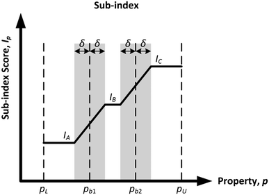
Based on the established inherent safety and health indexes, the allocation of sub-index scores is based on subjective scaling and weighting. The physical and chemical properties assessed in the sub-indexes are divided into subjective ranges, where each range is then assigned a distinct sub-index score depending on the authors' judgement. As mentioned in section 1, the main limitation of this method is the discontinuity at the boundary values, which is illustrated by the scenario in Fig. 1. The comparison of two property values near the same boundary value but located at different sub-ranges is not efficient as there exists discontinuity at the boundary value where the score switches abruptly from one value to another. This issue is addressed in this section, where the sub-index scores at the boundary value regions will be smoothened to ensure that there is continuity for the allocation of sub-index scores at any property value. The resulting general profile for the smoothened sub-index scores is shown in Fig. 4.
 |
| | Fig. 4 Smoothened sub-index scores. | |
In Fig. 4, the grey regions represent the smoothened regions where linear slopes are introduced to transit the scores from one sub-index value to another. The wideness of the smoothened region is determined by the value of δ. This value will identify the lower and upper bounds of the smoothened region for each boundary value. All smoothened regions should have a similar δ value for consistency purposes. To determine δ, a 10% margin of the property boundary values is applied. In general, a design factor of 10% is used for process flows to provide some flexibility in process operation.32 Therefore, a 10% safety/health factor is calculated for all boundary values in Fig. 4. Let us assume that the safety/health factors for pb1 and pb2 are δ1 and δ2, respectively. From Fig. 4, pb2 has a larger numerical value than pb1, so δ2 is larger than δ1. As mentioned previously, a similar δ value must be applied for all boundary values. In order to ensure that all boundary values can attain a minimum 10% factor, the selected δ value should take the largest value between δ1 and δ2. In this case, δ is equivalent to δ2. In other words, the δ value applied for a particular sub-index is the 10% factor of the largest boundary (numerical) value.
4.6 Disjunctive programming to assign sub-index scores
In this section, the algorithm to assign a sub-index score to a molecule depending on its property value is developed. Based on the modified sub-index in Fig. 4, the assigned sub-index score, Ip, is given by:| | 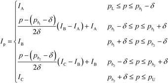 | (15) |
Based on eqn (15), the property value p is divided into five intervals. The sub-index score in each interval is defined by a distinct function. Thus, the sub-index score from the lower property value bound pL to the upper property value bound pU is not represented by a single continuous function. An algorithm known as disjunctive programming can be employed, which uses discontinuous functions to describe abrupt changes over a certain decision variable.33 This algorithm works by first determining which interval a specific property value p falls in. Once the interval is identified, its corresponding discontinuous score function will be applied to calculate the sub-index score to p. Binary integer variables are used to model these discontinuous functions. The Ip function in eqn (15) is converted to the following mixed-integer formulation using four binary integer variables (b1, b2, b3 and b4):
| | 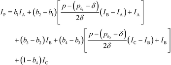 | (16) |
where the binary integer variables are subjected to the following criteria:
| |  | (17) |
| |  | (18) |
| |  | (19) |
| |  | (20) |
The binary integer variables in eqn (16) act as switches to only select a single score function at a time to determine the sub-index score. To ensure that the model allocates the correct value to the binary integer variables in order to satisfy criteria (17) to (20), the following constraints are also introduced:
| | | [pL − (pb1 − δ)]b1 < p − (pb1 − δ) ≤ [pU − (pb1 − δ)](1 − b1) | (21) |
| | | [pL − (pb1 + δ)]b2 < p − (pb1 + δ) ≤ [pU − (pb1 + δ)](1 − b2) | (22) |
| | | [pL − (pb2 − δ)]b3 < p − (pb2 − δ) ≤ [pU − (pb2 − δ)](1 − b3) | (23) |
| | | [pL − (pb2 + δ)]b4 < p − (pb2 + δ) ≤ [pU − (pb2 + δ)](1 − b4) | (24) |
4.7 Molecular group selection and structural constraints
In GCM, a molecule is formed by combining and bonding several molecular building groups, such as CH3, CH2, OH, CH3CO, CHNH2, etc. The full list for all possible first-order molecular building groups can be found in Hukkerikar et al.28,29 The selection of the appropriate molecular groups is dependent on the nature of the design problem. For example, molecular groups containing the nitrogen element must be selected for the design of amine-based molecules. Next, the octet rule of structural feasibility developed by Odele and Macchietto34 as shown by eqn (25) is included to ensure that the generated molecule does not contain free bonds:| |  | (25) |
where vi is the valence of group i, and Ni is the number of occurrences for first-order group i. The variable g is assigned a value of 1 or 0 for acyclic compounds and monocyclic compounds, respectively. In addition, the mathematical structural constraints proposed by Churi and Achenie35 are also introduced into the model to eliminate a combination of infeasible structures and to ensure that only a single molecular structure is produced.
4.8 Optimisation model formulation
In this stage, the optimisation model is developed by including all procedures from sections 4.1 to 4.7. The main design objective in this work is to maximise the product performance and to minimise the safety and health hazards posed by the molecules. Since there are multiple design criteria in this work, the CAMD problem has now become a multi-objective problem. In order to ensure that the two criteria do not compromise one another, a trade-off between them has to be considered. Optimal solutions can be generated from a multi-objective problem through the utilisation of a fuzzy optimisation algorithm. This approach is effective in solving multi-criteria problems without compromising either one of the criteria; thus, all design criteria can be optimised simultaneously. In order to achieve high product performance, the target properties selected as objective functions in section 4.1 will be optimised. On the other hand, the molecular safety and health level is measured by the total weighted index score ISHI,w in section 4.3 [eqn (10)]. High performance in terms of safety and health attributes can be attained by minimising ISHI,w. To apply fuzzy optimisation, first a degree of satisfaction for target property λp is assigned to each target property; while a degree of satisfaction for inherent safety and health λI is introduced into ISHI,w. Both λp and λI are represented by linear membership functions as shown in eqn (26) to (28):| | 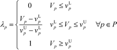 | (26) |
| | 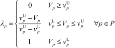 | (27) |
| |  | (28) |
where vLp and vUp are the property lower bound and upper bound, respectively, while IL and IU are the lower bound and upper bound of ISHI,w, respectively. Eqn (26) is only applied for the target property to be maximised, while eqn (27) is intended to minimise the target property. For eqn (26), the aim is to maximise the target property value. When Vp is lower than or equivalent to vLp, the aim is not satisfied; thus λp would be zero. The aim is achieved when Vp is higher than or equivalent to vUp; hence λp takes the value of one. In between vLp and vUp, a linear membership function is used where λp increases linearly from zero at vLp to one at vUp. The reverse trend is applied to eqn (27) to minimise the target property. Meanwhile, λI is calculated only by eqn (28) as ISHI,w is always minimised to reduce the intrinsic hazard level of the molecules.
Next, all λp and λI have to be maximised simultaneously to achieve a higher degree of satisfaction for all design criteria. In this work, the max–min aggregation method developed by Zimmermann36 is utilised to maximise all the degrees of satisfaction. This method assists in maximising the least satisfied degree of satisfaction, λ, to ensure that all λp and λI can be satisfied partially to at least the degree of λ. The following constraints are included for max–min aggregation, where the principal objective is to maximise the value of λ:
5. Case study: design of solvent to extract carotenoids from palm pressed fibre (PPF)
5.1 Design objective and problem formulation
Palm pressed fibre (PPF) is the residual by-product after the extraction of crude palm oil (CPO) from palm fresh fruit bunches (FFBs). The PPF is normally burned as fuel for power generation in palm oil mills37 or transported to the plantation for field mulching.38 However, Choo et al.39 found that the residual oil present in PPF contains a substantial amount of carotenoids (4000–6000 ppm), vitamin E (2400–3500 ppm), and sterols (4500–8500 ppm). Currently, hexane is the conventionally used solvent for extraction as it offers a high carotenoid extraction yield and has a convenient Tb, which is relatively low to limit heat consumption during carotenoid recovery but high enough to prevent much solvent losses during extraction.40 However, hexane is toxic to aquatic life, is highly flammable and may result in fatality if swallowed or inhaled.
In this case study, the objective is to identify a solvent that can replace hexane to extract carotenoids from the residual oil found in PPF. The solvent should be able to lower the energy requirement needed for evaporation. Thus, it must have a low boiling point (Tb) and low heat of vaporisation (Hv) so less energy is needed to heat the solvent to its Tb and subsequently vaporise it. In addition, carotenoids should have a high solubility in the developed solvent. The Hansen solubility parameter (HSP) can be applied to calculate the solubility of carotenoids in the solvent. The three parameters in the HSP are δd, δp and δh, which represent dispersion, polar and hydrogen bonding, respectively. Another parameter known as the distance of a solvent from the centre of the Hansen solubility sphere, Ra, can be calculated by eqn (31).41
| | | Ra2 = 4(δd,A − δd,B)2 + (δp,A − δp,B)2 + (δh,A − δh,B)2 | (31) |
In eqn (31), components A and B represent the solute (carotenoids) and solvent, respectively. A smaller Ra is desired as it indicates a greater affinity between the carotenoids and solvent. Next, the solvent must also achieve the desirable attributes for its safety and health aspects, such as low flammability and toxicity. These can be measured using the inherent safety and health sub-indexes selected in Table 3. The total weighted index score, ISHI,w in eqn (10), will be used to determine the inherent hazard level posed by the solvent. A low ISHI,w score is preferred for an inherently safer and healthier solvent.
Overall, the four main objective functions in this case study are to minimise Tb, minimise Hv, minimise Ra, and minimise ISHI,w. Since the conventionally used hexane is highly flammable and toxic to aquatic life, the flash point (Fp) and acute toxicity (96 h LC50 to fathead minnow) are selected as property constraints. The lower bound of Fp is set at −13.3 °C, which is 10 °C higher than that of hexane (−23.3 °C). As for acute toxicity LC50, the lower bound is set at 100 mg l−1, which indicates that the solvent is not harmful to the aquatic environment as defined by the United Nations' Globally Harmonised System of Classification and Labelling of Chemicals (GHS).
5.2 Safety and health assessment
As mentioned in section 4.2, the safety and health assessment of the solvent are measured using the selected safety and health sub-indexes that include flammability (IFL), explosiveness (IEX), viscosity (Iη), material phase (IMS), volatility (IV), exposure limit (IEL), and acute health hazard (IAH). All these sub-indexes are taken from the inherent safety and occupational health indexes found in the literature. When developing the sub-indexes, the range of the sub-index scores is assigned based on the importance of the specific sub-index to the plant safety6 and the magnitude of impacts resulting from chemical exposure.8 A more significant sub-index will be allocated to a larger scoring range. The scores of IFL and IAH are obtained from NFPA ratings, while scores for IMS, IV and IEL are taken from IOHI.8 Meanwhile, the sub-index values of IEX and Iη are referred from ISI6 and PRHI,7 respectively. Four sub-indexes (IFL, IEX, IEL and IAH) contain the largest scoring range of four, while two sub-indexes (Iη and IMS) have the smallest scoring range of two. It should be noted that both flammability and explosiveness are the crucial parameters affecting the safety factors of the chemical. For occupational health, the parameters of exposure limit and acute health hazard, which measure the toxicity of the chemical, will cause more significant health impacts on the plant workers.
Among the selected sub-indexes, their lowest scores vary from zero to one while their highest scores may vary from three to four. The scorings for all sub-indexes can be considered consistent as there are no sub-indexes with disproportionately high or low scores. In this work, the applied sub-index scores will be in the initial form. No score normalisation is carried out on the seven sub-indexes, as such a step will cause all sub-indexes to be considered to have equal importance. Eqn (10) is applied to calculate ISHI,w, where the seven sub-index scores are first sorted in descending order. The largest score is then multiplied by the largest weight, the second largest score is multiplied by the second largest weight, and so on. The proposed method to quantify the overall hazard of a solvent ensures that a particular sub-index displaying a higher hazard is penalised more; thus it has a larger impact on the ISHI,w score.
5.3 Identification of property prediction models
In section 5.1, the properties chosen as objective functions and constraints are Tb, Hv, Ra, Fp and LC50. Ra can be calculated from the three parameters of HSP: δd, δp and δh. Their corresponding property prediction methods must be identified in this stage to allow the model to estimate the property values. For Tb and Fp, their GCM models have been provided as shown in Table 7. Meanwhile, Hv, δd, δp and δh are estimated by methods presented by Hukkerikar et al.,29 while acute toxicity LC50 (96 h to fathead minnow) is predicted by a model introduced by Martin and Young.42
5.4 Smoothing sub-index scores
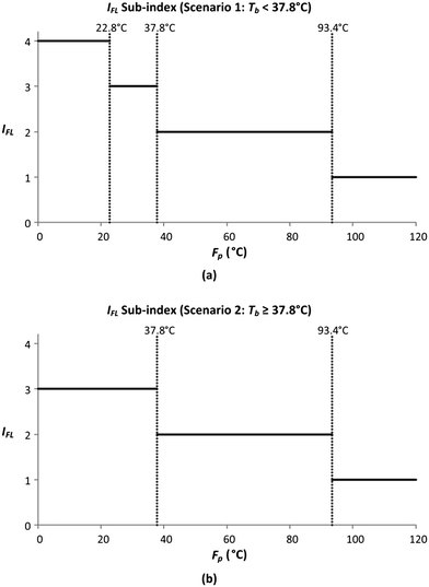
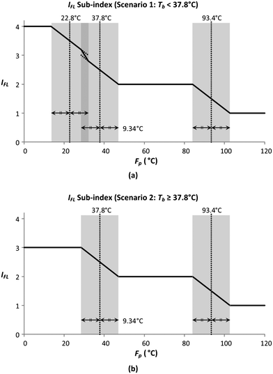
In this section, the smoothing of the flammability sub-index (IFL) is demonstrated. IFL evaluates the tendency of a material to burn in air. The allocation of IFL scores is shown in Table 8, where the two properties assessed by this sub-index include flash point (Fp) and boiling point (Tb). There are three boundary values for Fp (93.4 °C, 37.8 °C and 22.8 °C), while there is only a single boundary value for Tb (37.8 °C). Since there is only one Tb boundary, the IFL sub-index scores can be presented under two Tb scenarios, with the graphical representations shown in Fig. 5.
Table 8 Flammability (IFL) sub-index (NFPA)
| Factor |
Score information |
Penalty |
| Flammability, IFL |
Nonflammable |
0 |
|
F
p ≥ 93.4 °C |
1 |
|
F
p < 93.4 °C |
2 |
|
F
p < 37.8 °C |
3 |
|
F
p < 22.8 °C and Tb < 37.8 °C |
4 |
 |
| | Fig. 5 Sub-index scores of IFL when (a) Tb < 37.8 °C and (b) Tb ≥ 37.8 °C. | |
Fig. 5 shows the graphical illustration for the IFL sub-index under two Tb conditions. For both scenarios, the sub-index scores are similar above an Fp of 22.8 °C. However, the scores differ below an Fp of 22.8 °C, in which the scores increase to four in scenario 1 (Tb < 37.8 °C) while remaining at three in scenario 2 (Tb ≥ 37.8 °C). Thus, there will only be two Fp boundary values in scenario 2 (37.8 °C and 22.8 °C). At all boundary values, the IFL scores switch abruptly from one value to another. In this section, the scores at the boundary regions will be smoothened to address the discontinuity issue mentioned in section 4.5. The entire smoothing will be carried out in two parts; the first part will be conducted in terms of Fp, while the next part will be in terms of Tb. As mentioned previously, the boundary values for Fp are 93.4 °C, 37.8 °C and 22.8 °C. The 10% margins of the three boundary values are 9.34 °C, 3.78 °C and 2.28 °C, respectively. From the three margin values, the largest value, 9.34 °C, is chosen as the overall Fp margin. The selection of the largest margin value ensures that it attains at least a 10% factor of all boundary values. Next, a smoothing range is determined for each boundary value, where the lower bound is calculated by subtracting 9.34 °C from the boundary value, while the upper bound is determined by adding 9.34 °C to the boundary value. The smoothed regions are shown by the grey zones in Fig. 6. In these regions, the allocation of scores will be modified so that the scores can transit continuously from one value to another. For each region, a linear slope is introduced where it begins from the IFL score at the lower bound and decreases linearly to the IFL score at the upper bound. With the application of linear slopes, the smoothened IFL scores in terms of Fp are shown in Fig. 7. However, there exists an overlapping of two smoothing ranges (shown by the darker grey zone) in Fig. 7(a) as the lower bound for the 37.8 °C smoothing range is lower than the upper bound for the 22.8 °C range. As a result, two linear slopes (illustrated by the two dotted lines) are present in the overlapping range. However, any property value in the feasible property range can only be represented by a single score. Hence, a composite curve is used on the darker grey region as shown in Fig. 7(a) to merge the two linear slopes in which the score transits linearly from the higher score at the lower bound (28.46 °C) to the lower score at the upper bound (32.14 °C). Since the IFL scores are now smoothened in terms of Fp, the next step is to further smoothen the scores with regard to Tb.
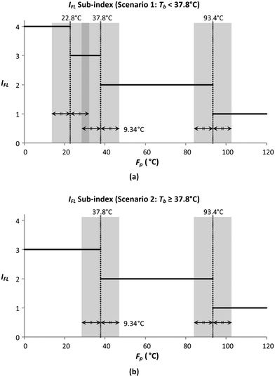 |
| | Fig. 6 Determining the range to smoothen in the IFL sub-index when (a) Tb < 37.8 °C; (b) Tb ≥ 37.8 °C. | |
 |
| | Fig. 7 Smoothened IFL scores when (a) Tb < 37.8 °C; (b) Tb ≥ 37.8 °C. | |
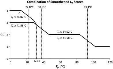
As shown by the two scenarios in Fig. 5 to 7, Tb has one boundary value of 37.8 °C. The margin value applied in Tb is the 10% factor of 37.8 °C, which is equivalent to 3.78 °C. The smoothened range for Tb is between 34.02 °C and 41.58 °C (37.8 ± 3.78 °C). Since scenario 1 is intended for a Tb value below 37.8 °C, while scenario 2 represents IFL scores for a Tb value above or equal to 37.8 °C; the scores in Fig. 7(a) now are applied for a Tb value below or equal to 34.02 °C, whereas the scores in Fig. 7(b) are utilised for a Tb value above or equal to 41.58 °C. The scores in Fig. 7(a) and (b) will now serve as the lower and upper bound values for the Tb smoothing range, respectively. Fig. 8 shows the combined IFL scores from Fig. 7(a) and (b).
 |
| | Fig. 8 Combined IFL scores. | |
From Fig. 8, at Fp below 32.14 °C, the IFL scores at or below the lower bound of the Tb smoothened range (34.02 °C) differ from the scores at or above the upper bound (41.58 °C). The two scores then converge at Fp of 32.14 °C, and the scores remain similar above that Fp value. Therefore, for a molecule with Fp above or equivalent to 32.14 °C, the IFL score is only dependent on its Fp regardless of the Tb value. For a molecule with Fp lower than 32.14 °C, if its Tb falls within the smoothing range (between 34.02 °C and 41.58 °C), an interpolation technique is required to determine its IFL score. First, both the Tb lower and upper bound scores are identified from Fig. 8 based on the Fp value of the molecule. The lower and upper bound scores now represent the IFL scores at Tb of 34.02 °C and 41.58 °C, respectively. Based on the estimated Tb of the molecule calculated by the GCM model in Table 8, the IFL score for the molecule can be determined through interpolation between the lower and the upper bound scores. For molecules with Tb below 34.02 °C or 41.58 °C, the scores are directly determined from the curves in Fig. 8. The overall smoothened IFL scores are summarised in Table 9. The other sub-indexes are also smoothened using the same technique, which are shown in the Appendix. IMS is the only sub-index that is not smoothened, since it measures the material state of the molecule without the need to divide the properties into sub-ranges. The IMS scores for gas, liquid and solid are 1, 2 and 3, respectively.
Table 9 Smoothened IFL scores
|
F
p (°C) |
I
FL,low (when Tb ≤ 34.02 °C) |
I
FL,up (when Tb ≥ 41.58 °C) |
|
F
p ≥ 102.74 °C |
1 |
1 |
| 84.06 °C ≤ Fp ≤ 102.74 °C |

|

|
| 47.14 °C ≤ Fp ≤ 84.06 °C |
2 |
2 |
| 32.14 °C ≤ Fp ≤ 47.14 °C |

|

|
| 28.46 °C ≤ Fp ≤ 32.14 °C |

|

|
| 13.46 °C ≤ Fp ≤ 28.46 °C |

|
3 |
|
F
p ≤ 13.46 °C |
4 |
3 |
Based on Table 9, the final IFL score can be determined by eqn (32):
| |  | (32) |
5.5 Molecular group selection and structural constraints
In this section, the selection of first-order molecular building blocks is based on the molecular structure of the conventionally used solvent to extract carotenoids. The chosen molecular groups include CH3, CH2, CH, C, OH, CH3CO, CH2CO, CH3O, CH2O, CHO, CH3COO, CH2COO, CH2 (cyclic), CH (cyclic), C (cyclic) and O (cyclic). To ensure that feasible molecules are synthesised, the structural constraints listed in section 4.7 are introduced into the model. The maximum number of molecular groups used to generate the molecules is set at 10. In addition, a constraint is also considered on molecular groups containing O:| | | nOH + nCH3CO + nCH2CO + nCH3O + nCH2O + nCHO + nCH3COO + nCH2COO + nO(cyc) ≤ 2 | (33) |
where nOH, nCH3CO, nCH2CO, nCH3CO, nCH2O, nCHO, nCH3COO, nCH2COO and nO(cyc) represent the number of occurrences of OH, CH3CO, CH2CO, CH3O, CH2O, CHO, CH3COO, CH2COO and O (cyclic) present in the molecule, respectively.
5.6 Optimisation model formulation
In the final stage, the four design objective properties are then converted into their respective property operator, Ωp, as shown in Table 10. Ωp is equivalent to the simple function f(p) for each target property p, which is exactly the left-hand side of eqn (1). The purpose of altering the form is to reduce the non-linearity equations in the model. The next step is to optimise the property operators of the four objective properties, which are ΩTb, ΩHv, ΩRa and ΩISHI,w. Since all four property operators are to be minimised, the linear membership functions given by eqn (27) and (28) are applied. The lower and upper bounds for the property operators must be identified by optimising each property operator one at a time. The boundary values are summarised in Table 10.
Table 10 Property operators and their lower and upper bounds
| Property p |
Ωp
|
Lower bound |
Upper bound |
|
T
b
|
exp(Tb/Tb0) |
3.0238 |
7.3889 |
|
H
v
|
H
v − Hv0 |
11.6891 |
36.8800 |
|
R
a
|
R
a
|
4.0542 |
15.8991 |
|
I
SHI,w
|
I
SHI,w
|
1.7463 |
2.6553 |
Then, λTb, λHv, λRa and λI are introduced into Tb, Hv, Ra and ISHI,w, respectively, for each of their linear membership functions as shown by eqn (34) to (37). The overall objective of the model is to maximise λ subjected to constraints (29) and (30). To generate multiple solutions, the integer cuts method is applied, whereby additional constraints are added into the model to synthesise alternate molecular structures.33
| |  | (34) |
| |  | (35) |
| |  | (36) |
| |  | (37) |
5.7 Results and discussion
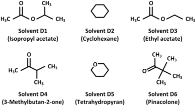
The top six solvents generated by the proposed optimisation model are shown in Fig. 9. The solvents can be categorised into esters (A1 and A3), ketones (A4 and A6) and monocyclic compounds (A2 and A5). Their estimated properties are shown in Table 11, while the sub-index values are summarised in Table 12. Solvent A1 is the best solution as it has a low ISHI,w and moderate Tb and Ra. When comparing the four objective properties individually, solvent A2 performs the best in terms of lowest Hv and Ra; while solvent A3 offers the lowest ISHI,w and Tb. In their work, Yara-Varón et al.40 showed that ethyl acetate (solvent A3 in this case study) offers a similar carotenoid extraction yield to that of hexane. Therefore, solvents A1, A2 and A5 with lower Ra than solvent A3 should exhibit better carotenoid extraction than hexane. Even though solvent A6 does not perform the best with regard to the four objectives, it still offers the highest Fp.
 |
| | Fig. 9 The generated solvents with their molecular structures. | |
Table 11 The six generated solvents with their properties
| Solvent |
λ
|
I
SHI,w
|
R
a
|
H
v (kJ mol−1) |
T
b (°C) |
F
p (°C) |
LC50 (mg l−1) |
| A1 |
0.697 |
1.957 |
7.432 |
34.32 |
86.2 |
9.6 |
114.6 |
| A2 |
0.687 |
2.031 |
4.147 |
29.08 |
80.1 |
−11.9 |
176.5 |
| A3 |
0.687 |
1.946 |
7.761 |
32.89 |
68.7 |
4.5 |
208.0 |
| A4 |
0.617 |
2.024 |
8.593 |
30.88 |
88.6 |
6.9 |
853.1 |
| A5 |
0.612 |
2.099 |
6.804 |
31.56 |
89.3 |
−2.6 |
875.7 |
| A6 |
0.597 |
2.049 |
8.208 |
32.07 |
109.5 |
14.0 |
521.9 |
Table 12 The six generated solvents with their sub-index scores
| Solvent |
I
FL
|
I
EX
|
Iη
|
I
MS
|
I
V
|
I
EL
|
I
AH
|
I
SHI
|
| A1 |
3 |
1 |
1 |
2 |
1 |
1.09 |
0.81 |
9.90 |
| A2 |
3 |
1 |
1 |
2 |
1 |
0.86 |
1.54 |
10.41 |
| A3 |
3 |
1 |
1 |
2 |
1 |
1.02 |
0.82 |
9.83 |
| A4 |
3 |
1 |
1 |
2 |
1 |
1.34 |
1.21 |
10.54 |
| A5 |
3 |
1 |
1 |
2 |
1 |
1.58 |
1.56 |
11.14 |
| A6 |
3 |
1 |
1 |
2 |
1 |
1.48 |
1.23 |
10.71 |
In terms of their individual sub-index scores, the difference between their safety and health performance is mainly contributed by IEL and IAH. These two sub-indexes measured the toxicity of chemicals, where IEL examines the chronic toxicity through inhalation, while IAH assesses acute toxicity through ingestion. ISHI in Table 12 is calculated by summing up the seven sub-index values of each solvent. Among the seven sub-index values in Table 12, the one with the largest penalty is IFL, which indicates that the solvents are easily flammable. In the event where a molecule with lower flammability is required, additional integer cuts are introduced to the optimisation model. The best solvent with a lower IFL score (less than or equal to 2) is 1-ethoxy-2-butanone with a λ value of 0.463, where its ISHI,w, Ra, Hv, Tb and Fp are equivalent to 2.144, 6.599, 37.15 kJ mol−1, 137.7 °C and 53.0 °C, respectively. Its Ra is lower than those of the top six solvents in Table 11, but it has a relatively high Tb and Hv, which means that more energy is needed to vaporise the solvent to recover carotenoids. Even though its IFL has an improved value of 2, its IEL score has worsened to 3, indicating that it has higher toxicity than the top six solvents. This also increases its overall inherent hazard level as demonstrated by its high ISHI,w.
The introduction of index smoothing and prioritisation in this paper enhances the representation of molecular safety and health performance through the calculation of the adjusted index score, ISHI,w. The improvement in safety and health measurement can be demonstrated by comparing the results in Table 12 with the calculation of ISHI,i of the six solvents by omitting both index smoothing and prioritisation. In other words, the initial index scoring schemes are used to calculate ISHI,i by summing up the sub-index scores without allocating weight factors to them. The calculated ISHI,i and the individual sub-index values are shown in Table 13. In Table 13, the IFL, IEX, Iη, IMS and IV scores of the six solvents remain unchanged, as their property values do not fall near the property boundaries of the five sub-indexes. As for IEL and IAH, the results in Table 12 show that the property values (PEL and LD50) of the solvents fall near the property boundaries or the edges of their respective property sub-ranges, so their IEL and IAH scores are not discrete values. In Table 13, all solvents but A5 have a similar IEL score of one, while the IAH scores of all solvents but A2 and A5 share the same value of one. Solvents A1, A3, A4 and A6 exhibit the lowest ISHI,i score of 10, while A2 and A5 possess higher hazard levels with total index scores of 11 and 12, respectively. As four solvents share the same ISHI,i, it is difficult to distinguish their inherent hazard level. This limitation is addressed with the proposed index smoothing and prioritisation in this paper, where the hazard level of each solvent can be calculated by ISHI,w as shown in Table 11.
Table 13 The six generated solvents (without index smoothing and prioritisation) with their sub-index scores
| Solvent |
I
FL
|
I
EX
|
Iη
|
I
MS
|
I
V
|
I
EL
|
I
AH
|
I
SHI,i
|
| A1 |
3 |
1 |
1 |
2 |
1 |
1 |
1 |
10 |
| A2 |
3 |
1 |
1 |
2 |
1 |
1 |
2 |
11 |
| A3 |
3 |
1 |
1 |
2 |
1 |
1 |
1 |
10 |
| A4 |
3 |
1 |
1 |
2 |
1 |
1 |
1 |
10 |
| A5 |
3 |
1 |
1 |
2 |
1 |
2 |
2 |
12 |
| A6 |
3 |
1 |
1 |
2 |
1 |
1 |
1 |
10 |
From the results, the smoothing of scores at property boundary offers a better comparison of hazard level among the solvents. For instance, the calculated ISHI,i values in Table 13 show that solvent A6 is less hazardous than A2. However, the calculated ISHI,w values in Table 11 demonstrate otherwise. This is because the PEL and LD50 (used to measure IEL and IAH, respectively) of solvent A6 are near the upper boundary (higher degree of hazard) of their respective sub-ranges; thus both its IEL and IAH scores as shown in Table 12 are penalised more than those in Table 13. The same happens to solvent A2 where its IAH score in Table 12 is penalised more than that in Table 13. Meanwhile, the PEL of solvent A2 falls near the lower boundary (lower degree of hazard) of its IEL sub-range; thus its IEL score as displayed in Table 12 is penalised less than that in Table 13. This results in the total ISHI,w of solvent A6 being greater than that of A2. The smoothing of scores also addresses the limitation of comparing two solvents with property values near one another but are separated by a sharp property boundary. For instance, the IEL scores of solvents A5 and A6 without index smoothing are two and one, respectively, in which their score difference is one. Their PEL values are close to one another but they are separated by a shape scoring edge, which results in their IEL scores being different. After the smoothing of sub-indexes, their IEL score difference is reduced to 0.1, as determined from Table 12. Hence, this revision of the sub-index scorings allows the comparison of molecular hazard among different alternatives to be done more accurately.
Meanwhile, the introduction of index prioritisation by assigning different weights to sub-indexes takes into account the severity of individual sub-index scores when quantifying the overall hazard level. To illustrate this improvement, the values of ISHI as shown in Table 12 are compared with their corresponding ISHI,w values in Table 11. It is noted that a higher ISHI value does not guarantee a larger ISHI,w value. Even though solvent A2 has a lower ISHI than solvent A4, it does not display the same relationship for their corresponding ISHI,w values. As the six solvents only have distinct IEL and IAH values, this discussion is focused only on these two sub-indexes. For solvent A2, its IAH value is higher than its IEL score, while it is the opposite for solvent A4. Since solvent A2 has a more severe IAH score (1.54) than the IEL score of solvent A4 (1.34), solvent A2 is penalised more with the application of eqn (10) to determine ISHI,w. Thus, the results prove that the adjusted index score takes into account the severity of each sub-index to help distinguish the safety and health attributes of the molecules.
In conclusion, the revision of the index scoring scheme improves the measurement and comparison of the inherent hazard level among molecules. First, the smoothing of scores at property boundaries in the sub-indexes can enhance the representation of molecular hazard level near the edges of the sub-range. In a specific sub-range, a molecular property that is near the upper edge with a higher hazard level will be penalised more, and vice versa. As a result, when this CAMD problem aims to minimise the total index score, the modification on the index scoring scheme allows the CAMD programming to opt for a solution that is closer to the lower edge (lower hazard) within a particular sub-range, as opposed to a solution with property at the upper edge or middle region of the sub-range. In another case, if there are two neighbouring solutions that may demonstrate a somewhat similar hazard level but are separated by the sharp scoring edge, the smoothing of scores at the boundary allows their score difference to be reduced. As the hazard levels of these two solutions are closer or slightly similar to each other, this allows the other design objectives to have a higher influence on the selection of the final optimal molecule. Meanwhile, the second improvement with index prioritisation allows the CAMD programming to consider the severity of each sub-index score when minimising ISHI,w. As a sub-index with a larger score is penalised to a greater extent, the CAMD programming will strive to minimise the severity of each sub-index score in order to generate a more conservative solution with respect to all safety and health sub-indexes. In general, the two discussed improvements allow a better reflection of molecular hazard level in order to synthesise an optimal molecule with enhanced quality in terms of property functionalities and safety and health performance.
Conclusions
In this work, inherent safety and health sub-indexes are integrated into the CAMD framework to measure the safety and health performance of the generated molecules. The main highlight is the development of an enhanced method to quantify the overall safety and health attributes of the molecules by applying an OWA operator to conditionally assign weight factors to the sub-indexes based on severity rank. Higher severity sub-index scores are given higher weights because these reflect the more critical or problematic features of the molecules. The AHP approach is employed to assist in determining the weight factors given to sub-indexes with different severity levels. In addition, a smoothing technique is developed to reduce the granularity and potential distortion caused by having discrete, stepwise hazard ranges. The smoothening region is determined by using a safety/health margin of 10%, and a linear transition slope is introduced for the score allocation. A case study has been considered to replace hexane for the extraction of carotenoids found in PPF. The results showed that the top six generated solvents offer high performance with respect to product functionality and the safety and health aspects. The adjusted index score ISHI,w as calculated by the OWA operator takes into account the severity of all sub-index scores to enhance the representation of overall hazard level as demonstrated by the solvents. For future work, the presented CAMD framework to design an optimal molecule with reduced risk can be extended to an integrated process–product design problem. Besides optimising the current design objectives (product functionalities and the molecular safety and health level), this problem also aims to optimise the process conditions and the process safety and health level. Instead of only applying the chemical-related sub-indexes, the inherent safety and health level of the process route can be examined by including the process-related sub-indexes. The proposed integrated process–product design framework can serve as a screening tool to design the optimal chemical and process operating conditions that demonstrate high product and process performance and favourable safety and health attributes.
Conflicts of interest
There are no conflicts of interest to declare.
Appendix: Smoothened inherent safety and health sub-indexes
Table A.1 Smoothened explosiveness (IEX) sub-index
| Factor |
Score information |
Penalty |
| Explosiveness, IEXS = (UEL–LEL) vol% |
0 ≤ S ≤ 13 |
1 |
| 13 ≤ S ≤ 27 |
(S − 13)/14 + 1 |
| 27 ≤ S ≤ 38 |
2 |
| 38 ≤ S ≤ 52 |
(S − 38)/14 + 2 |
| 52 ≤ S ≤ 63 |
3 |
| 63 ≤ S ≤ 77 |
(S − 63)/14 + 3 |
| 77 ≤ S ≤ 100 |
4 |
Table A.2 Smoothened viscosity (Iη) sub-index
| Factor |
Score information |
Penalty |
| Viscosity, Iη |
−1 ≤ log![[thin space (1/6-em)]](https://www.rsc.org/images/entities/char_2009.gif) η ≤ −0.1 η ≤ −0.1 |
1 |
−0.1 ≤ log![[thin space (1/6-em)]](https://www.rsc.org/images/entities/char_2009.gif) η ≤ 0.1 η ≤ 0.1 |
(log![[thin space (1/6-em)]](https://www.rsc.org/images/entities/char_2009.gif) η + 0.1)/0.2 + 1 η + 0.1)/0.2 + 1 |
0.1 ≤ log![[thin space (1/6-em)]](https://www.rsc.org/images/entities/char_2009.gif) η ≤ 0.9 η ≤ 0.9 |
2 |
0.9 ≤ log![[thin space (1/6-em)]](https://www.rsc.org/images/entities/char_2009.gif) η ≤ 1.1 η ≤ 1.1 |
(log![[thin space (1/6-em)]](https://www.rsc.org/images/entities/char_2009.gif) η − 0.9)/0.2 + 2 η − 0.9)/0.2 + 2 |
1.1 ≤ log![[thin space (1/6-em)]](https://www.rsc.org/images/entities/char_2009.gif) η ≤ 2 η ≤ 2 |
3 |
Table A.3 Smoothened volatility (IV) sub-index
| Factor |
Score information |
Penalty |
| Volatility, IV |
Liquid and gas |
|
|
T
b ≥ 165 °C |
0 |
| 165 °C ≥ Tb ≥ 135 °C |
(165 − Tb)/30 |
| 135 °C ≥ Tb ≥ 65 °C |
1 |
| 65 °C ≥ Tb ≥ 35 °C |
(65 − Tb)/30 + 1 |
| 35 °C ≥ Tb ≥ 15 °C |
2 |
| 15 °C ≥ Tb ≥ −15 °C |
(15 − Tb)/30 + 2 |
|
T
b ≤ −15 °C |
3 |
Table A.4 Smoothened exposure limit (IEL) sub-index
| Factor |
Score information |
Penalty |
| Exposure limit, IEL |
Vapour (ppm) |
|
log![[thin space (1/6-em)]](https://www.rsc.org/images/entities/char_2009.gif) PEL ≥ 3.3 PEL ≥ 3.3 |
0 |
2.7 ≤ log![[thin space (1/6-em)]](https://www.rsc.org/images/entities/char_2009.gif) PEL ≤ 3.3 PEL ≤ 3.3 |
(3.3 − log![[thin space (1/6-em)]](https://www.rsc.org/images/entities/char_2009.gif) PEL)/0.6 PEL)/0.6 |
2.3 ≤ log![[thin space (1/6-em)]](https://www.rsc.org/images/entities/char_2009.gif) PEL ≤ 2.7 PEL ≤ 2.7 |
1 |
1.7 ≤ log![[thin space (1/6-em)]](https://www.rsc.org/images/entities/char_2009.gif) PEL ≤ 2.3 PEL ≤ 2.3 |
(2.3 − log![[thin space (1/6-em)]](https://www.rsc.org/images/entities/char_2009.gif) PEL)/0.6 + 1 PEL)/0.6 + 1 |
1.3 ≤ log![[thin space (1/6-em)]](https://www.rsc.org/images/entities/char_2009.gif) PEL ≤ 1.7 PEL ≤ 1.7 |
2 |
0.7 ≤ log![[thin space (1/6-em)]](https://www.rsc.org/images/entities/char_2009.gif) PEL ≤ 1.3 PEL ≤ 1.3 |
(1.3 − log![[thin space (1/6-em)]](https://www.rsc.org/images/entities/char_2009.gif) PEL)/0.6 + 2 PEL)/0.6 + 2 |
0.3 ≤ log![[thin space (1/6-em)]](https://www.rsc.org/images/entities/char_2009.gif) PEL ≤ 0.7 PEL ≤ 0.7 |
3 |
−0.3 ≤ log![[thin space (1/6-em)]](https://www.rsc.org/images/entities/char_2009.gif) PEL ≤ 0.3 PEL ≤ 0.3 |
(0.3 − log![[thin space (1/6-em)]](https://www.rsc.org/images/entities/char_2009.gif) PEL)/0.6 + 3 PEL)/0.6 + 3 |
log![[thin space (1/6-em)]](https://www.rsc.org/images/entities/char_2009.gif) PEL ≤ −0.3 PEL ≤ −0.3 |
4 |
Table A.5 Smoothened acute health hazard (IAH) sub-index
| Factor |
Score information |
Penalty |
| Acute health hazard, IAH |
Oral rat LD50 (mg kg−1) |
|
log![[thin space (1/6-em)]](https://www.rsc.org/images/entities/char_2009.gif) LD50 ≥ 3.6311 LD50 ≥ 3.6311 |
0 |
3.0291 ≤ log![[thin space (1/6-em)]](https://www.rsc.org/images/entities/char_2009.gif) LD50 ≤ 3.6311 LD50 ≤ 3.6311 |
1.5147(3.6311 − log![[thin space (1/6-em)]](https://www.rsc.org/images/entities/char_2009.gif) LD50) LD50) |
2.9709 ≤ log![[thin space (1/6-em)]](https://www.rsc.org/images/entities/char_2009.gif) LD50 ≤ 3.0291 LD50 ≤ 3.0291 |
3.0294(3.0291 − log![[thin space (1/6-em)]](https://www.rsc.org/images/entities/char_2009.gif) LD50) + 0.9119 LD50) + 0.9119 |
2.3689 ≤ log![[thin space (1/6-em)]](https://www.rsc.org/images/entities/char_2009.gif) LD50 ≤ 2.9709 LD50 ≤ 2.9709 |
1.5147(3.0291 − log![[thin space (1/6-em)]](https://www.rsc.org/images/entities/char_2009.gif) LD50) + 1 LD50) + 1 |
2.0291 ≤ log![[thin space (1/6-em)]](https://www.rsc.org/images/entities/char_2009.gif) LD50 ≤ 2.3689 LD50 ≤ 2.3689 |
2 |
1.3689 ≤ log![[thin space (1/6-em)]](https://www.rsc.org/images/entities/char_2009.gif) LD50 ≤ 2.0291 LD50 ≤ 2.0291 |
1.5147(2.0291 − log![[thin space (1/6-em)]](https://www.rsc.org/images/entities/char_2009.gif) LD50) + 2 LD50) + 2 |
1.0291 ≤ log![[thin space (1/6-em)]](https://www.rsc.org/images/entities/char_2009.gif) LD50 ≤ 1.3689 LD50 ≤ 1.3689 |
3 |
0.3689 ≤ log![[thin space (1/6-em)]](https://www.rsc.org/images/entities/char_2009.gif) LD50 ≤ 1.0291 LD50 ≤ 1.0291 |
1.5147(1.0291 − log![[thin space (1/6-em)]](https://www.rsc.org/images/entities/char_2009.gif) LD50) + 3 LD50) + 3 |
log![[thin space (1/6-em)]](https://www.rsc.org/images/entities/char_2009.gif) LD50 ≤ 0.3689 LD50 ≤ 0.3689 |
4 |
Acknowledgements
The financial support from the Ministry of Higher Education, Malaysia through the LRGS Grant (Project Code: LRGS/2013/UKM-UNMC/PT/05) is gratefully acknowledged.
References
- M. Z. Abidin, R. Rusli, A. Buang, A. M. Shariff and F. I. Khan, J. Loss Prev. Process Ind., 2016, 44, 95 CrossRef.
- D. Mansfield and J. Hawksley, J. Cleaner Prod., 1998, 6, 147 CrossRef.
- T. A. Kletz, J. Soc. Chem. Ind., London, 1978, 278 Search PubMed.
-
T. A. Kletz, Cheaper, safer plants, or wealth and safety at work, The Institution of Chemical Engineers, Rugby, 1984 Search PubMed.
- D. W. Edwards and D. Lawrence, Chem. Eng. Res. Des., 1993, 71, 252 CAS.
-
A.-M. Heikkilä, Inherent safety in process plant design. An index based approach, Doctoral thesis, VTT Publications, Technical Research Centre of Finland, Espoo, 1999, vol. 384 Search PubMed.
- M. H. Hassim and D. W. Edwards, Process Saf. Environ. Prot., 2006, 84, 378 CrossRef CAS.
- M. H. Hassim and M. Hurme, J. Loss Prev. Process Ind., 2010, 23, 127 CrossRef.
- J. Y. Ten, M. H. Hassim, D. K. S. Ng and G. N. Chemmangattuvalappil, Chem. Eng. Sci., 2017, 159, 140 CrossRef CAS.
- R. Gani, Comput. Chem. Eng., 2004, 28, 2441 CrossRef CAS.
- J. Marrero and R. Gani, Fluid Phase Equilib., 2001, 183–184, 183 CrossRef CAS.
- A. P. Duvedi and L. E. K. Achenie, Chem. Eng. Sci., 1996, 51, 3727 CrossRef CAS.
- A. T. Karunanithi, L. E. K. Achenie and R. Gani, Chem. Eng. Sci., 2006, 61, 1247 CrossRef CAS.
-
S. Papadokonstantakis, S. Badr, K. Hungerbühler, A. I. Papadopoulos, T. Damartzis, P. Seferlis, E. Forte, A. Chremos, A. Galindo, G. Jackson and C. S. Adjiman, in Computer Aided Chemical Engineering, ed. F. You, Elsevier, Amsterdam, 2015, vol. 11, pp. 279–310 Search PubMed.
- O. Palma-Flores, A. Flores-Tlacuahuac and G. Canseco-Melchor, Energy, 2016, 99, 32 CrossRef CAS.
- V. Gerbaud, M. Teles Dos Santos, N. Pandya and J. M. Aubry, Chem. Eng. Sci., 2017, 159, 177 CrossRef CAS.
- M. Lampe, M. Stavrou, J. Schilling, E. Sauer, J. Gross and A. Bardow, Comput. Chem. Eng., 2015, 81, 278 CrossRef CAS.
- T. L. Saaty, Comput. Chem. Eng., 1994, 74, 426 Search PubMed.
-
T. L. Saaty and K. P. Kearns, Analytical planning: The organization of systems, Pergamon Press, Oxford, 1985 Search PubMed.
- T. L. Saaty, J. Math. Psychol., 1977, 15, 234 CrossRef.
-
T. L. Saaty, The Analytic Hierarchy Process, Mc-Graw-Hill, New York, 1980 Search PubMed.
- C. Palaniappan, R. Srinivasan and R. Tan, Ind. Eng. Chem. Res., 2002, 41, 6698 CrossRef CAS.
- Z. S. Xu and Q. L. Da, Int. J. Smart Sens. Intell. Syst., 2003, 18, 953 CrossRef.
- R. R. Yager, IEEE Trans. Syst. Man Cybern., 1988, 18, 183 CrossRef.
- R. R. Yager and A. Kelman, J. Intell. Fuzzy Syst., 1999, 7, 401 Search PubMed.
- M. T. Lamata, Int. J. Hybrid Intell. Syst., 2004, 19, 473 CrossRef.
- S. Boroushaki and J. Malczewski, Comput. Geosci., 2008, 34, 399 CrossRef.
- A. S. Hukkerikar, S. Kalakul, B. Sarup, D. M. Young, G. Sin and R. Gani, J. Chem. Inf. Model., 2012, 52, 2823 CrossRef CAS PubMed.
- A. S. Hukkerikar, B. Sarup, A. T. Kate, J. Abildkov, G. Sin and R. Gani, Fluid Phase Equilib., 2012, 321, 25 CrossRef CAS.
- E. Conte, A. Martinho, H. A. Matos and R. Gani, Ind. Eng. Chem. Res., 2008, 47, 7940 CrossRef CAS.
- J. Frutiger, C. Marcarie, J. Abildskov and G. Sin, J. Hazard. Mater., 2016, 318, 783 CrossRef CAS PubMed.
-
R. K. Sinnott, Chemical engineering, Volume 6: Chemical engineering design, Elsevier, Oxford, 2005 Search PubMed.
-
M. M. El-Halwagi, Sustainable design through process integration: Fundamentals and applications to industrial pollution prevention, resource conservation, and profitability enhancement, Elsevier, Oxford, 2012 Search PubMed.
- O. Odele and S. Macchietto, Fluid Phase Equilib., 1993, 82, 47 CrossRef CAS.
- N. Churi and L. E. Achenie, Ind. Eng. Chem. Res., 1996, 35, 3788 CrossRef CAS.
- H.-J. Zimmermann, Fuzzy Sets Syst., 1978, 1, 45 CrossRef.
- B. K. Neoh, Y. M. Thang, M. Z. M. Zain and A. Junaidi, Int. Food Res. J., 2011, 18, 769 CAS.
- H. L. N. Lau, Y. M. Choo, A. N. Ma and C. H. Chuah, J. Food Eng., 2008, 84, 289 CrossRef CAS.
- Y. M. Choo, S. C. Yap, C. K. Ooi, A. N. Ma, S. H. Goh and A. S. H. Ong, J. Am. Oil Chem. Soc., 1996, 73, 599 CrossRef CAS.
- E. Yara-Varón, A. S. Fabiano-Tixier, M. Balcells, R. Canela-Garayoa, A. Bily and F. Chemat, RSC Adv., 2016, 6, 27750 RSC.
-
C. M. Hansen, Hansen solubility parameters: A user's handbook, CRC Press, Boca Raton, 2007 Search PubMed.
- T. M. Martin and D. M. Young, Chem. Res. Toxicol., 2001, 14, 1378 CrossRef CAS PubMed.
|
| This journal is © The Royal Society of Chemistry 2018 |
Click here to see how this site uses Cookies. View our privacy policy here.  a and
Nishanth G.
Chemmangattuvalappil
 *a
*a


![[thin space (1/6-em)]](https://www.rsc.org/images/entities/char_2009.gif) PEL
PEL![[thin space (1/6-em)]](https://www.rsc.org/images/entities/char_2009.gif) LD50 − ALD50 − BLD50Mw
LD50 − ALD50 − BLD50Mw![[thin space (1/6-em)]](https://www.rsc.org/images/entities/char_2009.gif) η
η


![[thin space (1/6-em)]](https://www.rsc.org/images/entities/char_2009.gif) η ≤ −0.1
η ≤ −0.1![[thin space (1/6-em)]](https://www.rsc.org/images/entities/char_2009.gif) η ≤ 0.1
η ≤ 0.1![[thin space (1/6-em)]](https://www.rsc.org/images/entities/char_2009.gif) η + 0.1)/0.2 + 1
η + 0.1)/0.2 + 1![[thin space (1/6-em)]](https://www.rsc.org/images/entities/char_2009.gif) η ≤ 0.9
η ≤ 0.9![[thin space (1/6-em)]](https://www.rsc.org/images/entities/char_2009.gif) η ≤ 1.1
η ≤ 1.1![[thin space (1/6-em)]](https://www.rsc.org/images/entities/char_2009.gif) η − 0.9)/0.2 + 2
η − 0.9)/0.2 + 2![[thin space (1/6-em)]](https://www.rsc.org/images/entities/char_2009.gif) η ≤ 2
η ≤ 2![[thin space (1/6-em)]](https://www.rsc.org/images/entities/char_2009.gif) PEL ≥ 3.3
PEL ≥ 3.3![[thin space (1/6-em)]](https://www.rsc.org/images/entities/char_2009.gif) PEL ≤ 3.3
PEL ≤ 3.3![[thin space (1/6-em)]](https://www.rsc.org/images/entities/char_2009.gif) PEL)/0.6
PEL)/0.6![[thin space (1/6-em)]](https://www.rsc.org/images/entities/char_2009.gif) PEL ≤ 2.7
PEL ≤ 2.7![[thin space (1/6-em)]](https://www.rsc.org/images/entities/char_2009.gif) PEL ≤ 2.3
PEL ≤ 2.3![[thin space (1/6-em)]](https://www.rsc.org/images/entities/char_2009.gif) PEL)/0.6 + 1
PEL)/0.6 + 1![[thin space (1/6-em)]](https://www.rsc.org/images/entities/char_2009.gif) PEL ≤ 1.7
PEL ≤ 1.7![[thin space (1/6-em)]](https://www.rsc.org/images/entities/char_2009.gif) PEL ≤ 1.3
PEL ≤ 1.3![[thin space (1/6-em)]](https://www.rsc.org/images/entities/char_2009.gif) PEL)/0.6 + 2
PEL)/0.6 + 2![[thin space (1/6-em)]](https://www.rsc.org/images/entities/char_2009.gif) PEL ≤ 0.7
PEL ≤ 0.7![[thin space (1/6-em)]](https://www.rsc.org/images/entities/char_2009.gif) PEL ≤ 0.3
PEL ≤ 0.3![[thin space (1/6-em)]](https://www.rsc.org/images/entities/char_2009.gif) PEL)/0.6 + 3
PEL)/0.6 + 3![[thin space (1/6-em)]](https://www.rsc.org/images/entities/char_2009.gif) PEL ≤ −0.3
PEL ≤ −0.3![[thin space (1/6-em)]](https://www.rsc.org/images/entities/char_2009.gif) LD50 ≥ 3.6311
LD50 ≥ 3.6311![[thin space (1/6-em)]](https://www.rsc.org/images/entities/char_2009.gif) LD50 ≤ 3.6311
LD50 ≤ 3.6311![[thin space (1/6-em)]](https://www.rsc.org/images/entities/char_2009.gif) LD50)
LD50)![[thin space (1/6-em)]](https://www.rsc.org/images/entities/char_2009.gif) LD50 ≤ 3.0291
LD50 ≤ 3.0291![[thin space (1/6-em)]](https://www.rsc.org/images/entities/char_2009.gif) LD50) + 0.9119
LD50) + 0.9119![[thin space (1/6-em)]](https://www.rsc.org/images/entities/char_2009.gif) LD50 ≤ 2.9709
LD50 ≤ 2.9709![[thin space (1/6-em)]](https://www.rsc.org/images/entities/char_2009.gif) LD50) + 1
LD50) + 1![[thin space (1/6-em)]](https://www.rsc.org/images/entities/char_2009.gif) LD50 ≤ 2.3689
LD50 ≤ 2.3689![[thin space (1/6-em)]](https://www.rsc.org/images/entities/char_2009.gif) LD50 ≤ 2.0291
LD50 ≤ 2.0291![[thin space (1/6-em)]](https://www.rsc.org/images/entities/char_2009.gif) LD50) + 2
LD50) + 2![[thin space (1/6-em)]](https://www.rsc.org/images/entities/char_2009.gif) LD50 ≤ 1.3689
LD50 ≤ 1.3689![[thin space (1/6-em)]](https://www.rsc.org/images/entities/char_2009.gif) LD50 ≤ 1.0291
LD50 ≤ 1.0291![[thin space (1/6-em)]](https://www.rsc.org/images/entities/char_2009.gif) LD50) + 3
LD50) + 3![[thin space (1/6-em)]](https://www.rsc.org/images/entities/char_2009.gif) LD50 ≤ 0.3689
LD50 ≤ 0.3689
