Selecting optimal features from Fourier transform infrared spectroscopy for discrete-frequency imaging

Abstract

Tissue histology utilizing chemical and immunohistochemical labels plays an important role in biomedicine and disease diagnosis. Recent research suggests that mid-infrared (IR) spectroscopic imaging may augment histology by providing quantitative molecular information. One of the major barriers to this approach is long acquisition time using Fourier-transform infrared (FTIR) spectroscopy. Recent advances in discrete frequency sources, particularly quantum cascade lasers (QCLs), may mitigate this problem by allowing selective sampling of the absorption spectrum. However, DFIR imaging only provides a significant advantage when the number of spectral samples is minimized, requiring a priori knowledge of important spectral features. In this paper, we demonstrate the use of a GPU-based genetic algorithm (GA) using linear discriminant analysis (LDA) for DFIR feature selection. Our proposed method relies on pre-acquired broadband FTIR images for feature selection. Based on user-selected criteria for classification accuracy, our algorithm provides a minimal set of features that can be used with DFIR in a time-frame more practical for clinical diagnosis.

---

Histological studies generally rely on chemical stains for characterization and diagnosis. However, chemical staining is destructive to the sample and sensitive to variations in tissue preparation and imaging protocols. While methods have been proposed to normalize stained images,¹ this remains a complex problem in automated histology. Mid-infrared (IR) spectroscopic imaging has the potential to address these problems by providing quantitative molecular information to augment current practice.² A significant body of recent work focuses on using Fourier transform infrared (FTIR) imagery to perform tissue characterization and classification.^3,4 FTIR image classification has been successfully applied to multiple disease types, such as Barrett's esophagus⁵ as well as a variety of cancers including breast,^6–8 cervix,⁹ colon,¹⁰ liver,¹¹ lung,¹² and prostate.^13–15 However, FTIR spectroscopic imaging has several limitations that preclude clinical translation, including long image acquisition time and the need to manage the large data size. For example, collecting an image representing a 1 cm² surgical resection at a resolution comparable to standard histology requires ≈500 GB. Prior knowledge of the necessary features would allow for dimension reduction after acquisition but before data storage, dramatically reducing the resulting data size. However, FTIR image acquisition time is much more difficult to reduce. Most methods to reduce image acquisition time, such as reducing spectral resolution or image co-additions, result in degradation of the image and spectral quality. However, prior information about the necessary spectral features would allow for optimization of these parameters.

Recent attempts to address these issues include the use of discrete frequency infrared (DFIR) imaging. DFIR allows the collection of individual wavelengths using either a tunable quantum cascade laser (QCL) source^16,17 or filter bank.¹⁸ However, sparse collection of spectral features is only possible if the required bands are known a priori. In this study, we address the problem of developing an optimized search for finding bands that are important for multi-class histological labeling of biological tissue. TMA cores are imaged using FTIR to generate data for our search. Due to the nature of DFIR images, feature selection methods, such as principal component analysis (PCA), and independent component analysis (ICA),¹⁹ and vertex component analysis (VCA)²⁰ are impractical, since they result in features that have broad spectral support. Our focus is on feature selection, since the resulting features can be translated to DFIR image acquisition, significantly reducing the time required for image acquisition and eliminating the need for later dimension reduction. We compare the results of the proposed GPU-based genetic algorithm using linear discriminant analysis (GA-LDA) with other prominent feature selection methods, demonstrating that this technique provides comparable results to feature extraction methods. Finally, we show that these features provide excellent accuracy when applied to DFIR images acquired using a commercial QCL-based imaging system.

1 Background

Vibrational spectroscopic imaging provides label-free molecular specificity by measuring absorbance in the mid-infrared range (2.5–25 μm). Classification using vibrational spectra has been extensively explored in biomedical imaging, with a particular focus on Fourier-transform infrared (FTIR) spectroscopy.^3,21,22 FTIR is particularly promising, due to the combination of a large absorbance signal and molecular specificity. In addition, FTIR has existing protocols that can potentially fit within the standard pathology pipeline²³ and even map FTIR spectra to labels familiar to histologists trained in a traditional setting.²⁴

FTIR spectroscopy usually relies on illuminating a sample using a broad-band (globar) source that is passed through an interferometer to collect an interferogram. Individual wavelengths are separated using a Fourier transform. Data rate is usually limited by the low intensity of benchtop broadband IR sources, combined with the limited size of compatible mercury cadmium telluride (MCT) focal plane array (FPA) detectors. Data collection is often followed up with noise and dimension reduction algorithms to further improve SNR and mitigate the problems associated with a large number of features. This suggests that current histological classification relies on a sparse spectrum, containing a limited number of important components necessary for classification.^25,26 Consequently, DFIR imaging may provide an alternative to FTIR imaging by allowing direct imaging of the sparse features necessary for classification and thereby mitigating problems with both acquisition and data size.²⁷ DFIR instruments coupled with narrow bandwidth quantum cascade lasers can image a tissue sample at spectral bands optimal for classification.²⁸ QCL-based instruments provide a coherent source, allowing the use of high-resolution bolometer detectors and better optics.¹⁷ With a priori knowledge of important features, it is possible to limit collection to the most informative bands for classification.

Raw hyperspectral imagery has thousands of spectral features, making them difficult to classify due to memory constraints and prone to over-fitting. Dimension reduction is generally used to provide a more concise spectral representation. The most common approaches project the spectra into a new space and sort them based on some standardized score. The highest scored features are used in classification. Two broad types of dimension reduction are used: projection-based feature extraction and feature selection.²⁹ In projection-based feature extraction, basis functions are computed from high dimensional data using either an unsupervised or supervised approach. Principal component analysis (PCA) and Linear discriminant analysis (LDA), with some variations, are widely used feature extraction methods.^30,31 In the case of PCA, features are sorted based on the amount of variance accounted for in each projection,^32,33 whereas LDA relies on supervised data to optimize linear separability.

Feature selection methods rely on known sparsity within the spectrum, and common methods include the least absolute shrinkage and selection operator (LASSO), sequential feature selection method minimum Redundancy Maximum Relevance (mRMR)³⁴ and evolutionary learning genetic algorithms. As discussed earlier, our goal is to select features so that we can take advantage of DFIR imaging for fast tissue characterization.

Hyperspectral images collected using FTIR also undergo preprocessing, such as baseline correction and normalization, in order to mitigate spectral features correlated with sample structure and scattering.²³ The proposed feature selection is performed on preprocessed FTIR images of tissue microarrays from multiple patient biopsies. A GA is designed to perform supervised feature selection, relying on mRMR as an initialization step and LDA as an optimization metric. This method is ideal for optimizing features across multiple classes and classifiers. We then validate the selected features, demonstrating that the GA-LDA approach provides results are of comparable quality to feature extraction while also being compatible with DFIR imaging. Finally, we validate this approach for QCL-based images of tissue biopsies collected using a commercial DFIR imaging system (Fig. 1).

Fig. 1 Flowchart for a general genetic algorithm (GA). An initial population is created using randomized sampling or some preliminary guess. At every iteration i ≤ I_max, the population is evaluated using a fitness function. Features are sorted based on their score, and a new population i + 1 is created from the optimal features. Variability is introduced using mutation to reduce over-fitting. Our proposed algorithm uses mRMR for initialization and Fisher's ratio for evaluation.

2 Materials and methods

All samples were from formalin fixed paraffin embedded (FFPE) tissue microarrays (TMAs) purchased from US Biomax and AMSBio. TMAs included normal and tumor biopsies from breast, kidney, bone, and liver. Patient and sample variety aids in addressing variance due to biodiversity and demonstrates applicability across a broad range of tissue types.³⁵ FFPE TMA blocks were cut into 5 μm thick sections, with adjacent sections placed on alternate glass and BaF₂ slides. All samples are baked at 45 °C for 1.5 h and undergo three xylene washes (3 min each) for deparaffinization, followed by three ethanol washes (1 min each) with 100%, 90%, and 75% concentration. BaF₂ slides were first imaged using an FTIR microscope (Cary 620, Agilent) with a 15× 0.65NA objective mapped to a 128 × 128 pixel FPA, providing a pixel size of ≈5 μm. Data was collected in the spectral range of 1000–3900 cm⁻¹ with a spectral resolution of 8 cm⁻¹.

The FTIR images were annotated by an experienced pathologist based on adjacent histological staining. Histological stains included hematoxylin & eosin (H&E) and Masson's trichrome for all samples. This allowed us to examine general tissue structure and annotate collagen and smooth muscle. Since the breast images were the most histologically complex, additional immunohistochemical labels were used to confirm tissue phenotype. These include cytokeratin 19 for differentiating between epithelium and necrosis, as well as alpha smooth muscle actin (αSMA) and vimentin for identifying myofibroblasts.

Labels focused on cancer-relevant phenotypes ranging from 4–7 classes types, depending on tissue type. Feature selection was performed using the proposed GPU-based GA-LDA optimization method (section 1). Our goal was to select features from FTIR data that provide high-quality classification with finite support optimal for DFIR imaging. Since current commercial QCLs are limited to the 920–1800 cm⁻¹ range, analysis was limited to this window for feature selection. After the desired number of features were selected, the annotated data was then used to train a Random Forest³⁶ classifier. For random forest classifier 100 number of trees are selected and at each decision split of a tree default number of features are selected which is square root of total number of features used for classification. Ensemble treebagger is executed with parallel mode option using 6 threads on CPU. Classifier performance was validated on independent TMA images. When training and validating classifiers, it is crucial to ensure that individual cores are not shared by the training and validation sets. In such a case, any deviation in focus will cause chemical information to smear across pixels resulting in inflated performance measurements.

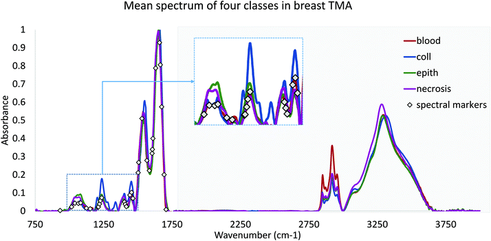
Finally, we validated the performance of our features in practice using DFIR images. TMA's were re-imaged using a QCL-based DFIR imaging system (SPERO, Daylight Solutions) with a 12.5× 0.7NA refractive objective. Data was collected at discrete frequencies specified by the proposed optimization algorithm. Note that all features require corresponding baseline points and a normalization band. Since the FTIR data were normalized to Amide I (1650 cm⁻¹), each spectral feature would require at most two adjacent baseline bands. However, note that optimized features often share similar peaks and can share baseline points (Fig. 2). Rubber band baseline correction was used,²³ combined with normalization to Amide I peak. No other noise reduction or pre-processing was applied. No other noise reduction or pre-processing was applied.

Fig. 2 Mean FTIR spectra of four classes from annotated breast biopsies. Spectra are normalized and baseline corrected. Features are selected by the GA-LDA algorithm from the fingerprint region only (≈900 cm⁻¹ to 1800 cm⁻¹), in order to ensure compatibility with DFIR imaging systems.

2.1 Feature selection

Feature extraction methods such as PCA, ICA, and VCA are routinely used in FTIR image analysis for dimension reduction and chemometrics. While these methods can capture molecular information in a relatively small number of features, the resulting basis functions have broad support. Therefore, use of traditional feature extraction requires collection of the entire spectrum. Our goal is to instead rely on feature selection by limiting features that can be discretely measured with a tunable DFIR imaging system. Since we know a priori that most of these features contain redundant information, we instead use sampling-based approaches to minimize the number of evaluation. Our approach utilizes two optimization methods for feature selection: minimum redundancy maximum relevance (mRMR) and a genetic algorithm (GA). This approach is further optimized to create an optimal supervised feature selection algorithm designed for DFIR image classification (Fig. 3).

Fig. 3 (a) H&E stained tissue cores from TMA AMS802. (b) FTIR and (c) DFIR imaged tissue core from breast TMA BR802 adjacent to H&E stained tissue section, classified into four classes: blood, collagen, epithelium and necrosis. Classification uses 20 features selected with GA-LDA from FTIR imaged data.

2.1.1 Minimum redundancy maximum relevance (mRMR). mRMR is a supervised incremental feature selection algorithm that searches for features based on maximum relevance and minimum redundancy criteria.³⁷ This technique has been successfully used with FTIR data to reduce the number of bands considered in histopathological classification.³⁴ We are given a sample matrix F ∈ [Doublestruck R]^S×B, where S is the number of samples (pixels) and B is the number of features (bands) along with a set of C class indices c ∈ [Doublestruck Z]^S ∈ [1,C] corresponding to each sample and a desired number of features N. We wish to calculate a set of indices n ∈ [Doublestruck Z]^N corresponding to the best features in the training set F.

The mRMR algorithm extracts these features iteratively by optimizing the following condition for each j ∈ [1,…, N]:

where B = [1,…, B] is the set of all feature indices and n_i is the set of i previously computed features. The mutual information function I(·) is given by:

The mRMR algorithm performs an iterative search for optimal features, which are added to the final set n until the desired N features are identified (Algorithm 1). A feature index j corresponding to feature x_j in F is added to the final feature set if it exhibits: (i) maximum mutual information with the distribution of class indices in the training set, and (ii) minimum mutual information with previously selected features in n.

Algorithm 1 Algorithm for calculating the maximum relevance minimum redundancy (mRMR) feature set

Input: F ∈ [Doublestruck R]^S×B c ∈ [Doublestruck Z]^S N

Output: n ∈ [Doublestruck Z]^N

1: n = ∅

2: while |n| ≤ Ndo //while features <N

3:  j = 1

4:  whilej ≤ Bdo

5:   find j such that eqn (1) is maximized

6:   append j to n

7:  end while

8: end while

While mRMR algorithm runs in O(n²) (quadratic) time and is deterministic, this efficiency comes in the form of a greedy algorithm that limits sampling to an extremely small subspace. Optimization is constrained by previously selected features, which are likely sub-optimal. Adding additional features increases redundancy rather than improving classification accuracy – particularly for complex data.

2.1.2 GA-LDA. In order to select discrete wavelengths for classification, we use a genetic algorithm (GA)³⁸ to optimize feature selection based on a linear discriminant analysis (LDA) cost function.^39,40 A GA is an evolutionary optimization method inspired by natural selection. Since our goal is to maximize classification accuracy while minimizing DFIR image acquisition time, we use a GA to select optimal feature sets for a range of feature numbers. This allows a user to select the optimal balance between classification accuracy and DFIR image acquisition time.

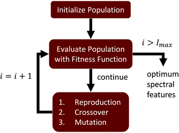
Given a number of desired features N ∈ [Doublestruck Z], a single GA attempts to select an optimal set of wavelengths that maximize classification accuracy (Fig. 1). Our GA is first initialized with a set of probable solutions, referred to as the initial population, one of the probable solution is initialized using mRMR feature selection algorithm (section 1).

Input to the genetic algorithm is a two dimension feature matrix loaded from the original three dimension hyperspectral image. In this feature matrix, rows are pixels (samples) and columns are spectral features (bands). Over the course of G generations, our GA attempts to select an optimal feature set given a specified number of target features N. Each genome is a vector of size N, and each element of a genome is a spectral feature index from the input feature matrix F. The population matrix P is a matrix P ∈ [Doublestruck R]^P×N, where N number of features to be selected using GA-LDA algorithm and P is the population size, which determines how densely the feature subspace is sampled. Increasing P and G provide additional optimization at the cost of processing time, where P is user-specified and G is determined by a stopping condition described later.

At each generation g ∈ [0, G), all genomes from the current population are evaluated using an optimization function and ranked into R according to their fitness values V_g. Based on these rankings, three population evolution operations are performed on current population reproduction, crossover, and mutation to generate next generation population. This evolutionary search for optimal spectral features continues until a stopping criteria is met. In our algorithm stopping criteria is until execution it reaches to maximum number of generations G_max or improvement in fitness value of best highest ranked genome is stalled over G_s number of generations, here G_max and G_s are user defined numbers and G_s ≪ G_max.

Algorithm 2 Algorithm for selecting optimal feature subset using evolutionary search

Input: F ∈ [Doublestruck R]^S×B c ∈ [Doublestruck Z]^S N P

Output: n ∈ [Doublestruck Z]^N

1: G = 0

2: initialize population matrix P₀ ∈ [Doublestruck Z]^P×N

3: whileG < G_maxdo

4:  for each genome p ∈ [0, P) do

5:   evaluate genome fitness T̂[p]

6:  end for

7:  generate a sorted list of genomes α ∈ [0, P) based on T̂

8:   ex. α[0] = argmax_jT̂ [ j] and α[P − 1] = argmin_jT̂ [ j]

9:  if genome α[0] meets stopping criteria then

10:   return genome α[0]

11:  end if

12:  Generate new population P_G+1:

13:   reproduce genomes α[0] to α[n_r − 1]

14:   generate new genomes for α[n_r] to α[N − 1] by crossover

15:   randomly mutate n_m genomes in α[n_r] to α[N − 1]

16:  G = G + 1

17: end while

18: return genome α[0]

Evolutionary learning is based on natural selection, such that the highest ranked n_r < P genomes are preserved (reproduction) in next generation population G + 1. The remaining n_c = P − n_r genomes are updated by performing the crossover operation on current generation genomes. Crossover is performed on parent genomes using a tournament selection method. A subset of t_s parent genomes are selected from the current generation population P_G from the subset of n_c genomes that are not reproduced. Each pair of selected parents go through crossover to generate a new genome. Once n_c new genomes are generated in P_next then with random sampling n_m genomes from n_c crossovered genomes go through mutation.

For example, assume a population of P = 20 genomes with n_r = 2 and n_m = 10. The next generation will consist of the n_r = 2 optimal genomes from the previous generation, while the remaining n_c = 18 genomes will consist of permutations of the previous sub-optimal genomes. This crossover is performed by selecting parents from the sub-optimal n_c = 18 genomes from the previous generation. Out of these n_c = 18 crossover genomes, n_m = 10 undergo random mutations. This random selection is done by using mutation probability, genomes for which randomly generated probability is greater than user defined mutation probability will go through mutation. In mutation operation, one or more genome entries are altered based on randomly generated probability to any feature index from the entire spectral range of input data. Mutation is important for GA as it avoids getting trapped in a local minimum.

Once a new population is obtained, the next generation is evaluated (Algorithm 2) until one of two conditions are met: (i) a maximum number of generations G_max is exceeded or (ii) there is less than ε improvement in the fitness score of the best genome.

The fitness function is a key component of the GA. Since statistical classifiers are frequently used in chemometrics, we focus on the linear separability of target classes using linear discriminant analysis (LDA). This is a supervised method for finding a linear transformation which will maximize inter class separability and minimize intra class variability. We implement Fisher's criterion as a generalized eigenvalue decomposition problem.⁴¹ The proposed GA finds a feature subset using LDA such that the projected data will have maximum between class scatter S_b and minimum within class scatter S_w. At each generation, the optimal transformation matrix T̂ for the current feature subset is computed by maximizing Fisher's ratio:

where the between class scatter S_b is the covariance of class means, and the within class scatter S_w is sum of variance for all classes:

2.2 GPU implementation

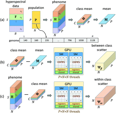
The major limitation of GA optimization is computational complexity, requiring ≈27 hours to select 50 features from 200k samples (1626 bands each) to separate 7 classes. mRMR uses a greedy approach, which significantly increases speed at the cost of getting trapped in local minima. Most feature extraction algorithms achieve optimal performance, however require access to the entire feature set for classification. Neither approach is viable for clinical application of DFIR, where image acquisition time and accuracy must be optimized. These two competing requirements necessitate the use of a computationally complex optimization. We elected to use the GA optimization approach because it is highly data parallel. The fitness of each genome can be tested independently using the same set of instructions. This makes it highly amenable to acceleration on GPUs, which are inexpensive and readily available in most research labs.

We first load the hyperspectral image as a feature matrix F ∈ [Doublestruck R]^S×B (Fig. 5a), where S is the number of samples (pixels) and B is the number of available bands (features). A population matrix P ∈ [Doublestruck R]^P×N is constructed with P genomes containing N features. The number of features N is tested for a user-specified range in order to determine the trade-off between accuracy and feature number. The population size P determines the number of permutations tested for each generation.

Fig. 4 Feature selection using mRMR vs. genetic algorithms. (a) The first iteration of mRMR selects an optimal feature testing all possibilities for maximum mutual information. Optimization of all features would be impractical. (b) Following iterations of mRMR are constrained by the initial feature(s) and therefore miss optimal values that deviate from this constrained subspace. Genetic algorithms introduce mutations that allow sampling outside of the subspace, reducing over-fitting.

Fig. 5 GPU implementation of GA-LDA. (a) Input tensors are generated for all genomes using the CPU. The population, represented as feature indices, is used to generate a phenome tensor containing feature values for the population. The mean and class means are then computed. (b and c) The between class scatter Ψ_β and within class scatter Ψ_ω are calculated on the GPU in parallel, significantly reducing the computational complexity. The final results are exported to the CPU for eigendecomposition using LAPACK.

While a CPU-based algorithm requires each genome to be evaluated sequentially, our GPU-based approach compiles the entire population into a phenotype tensor H ∈ [Doublestruck R]^S×N×P, where each value in H is a feature value corresponding to the appropriate sample and genome index from the current population matrix P. This phenome matrix H is then used to calculate the class mean tensor Φ ∈ [Doublestruck R]^C×N×P and the global mean matrix M ∈ [Doublestruck R]^N×P (Fig. 5a). These tensors are stored in GPU memory and used to calculate the between class scatter Ψ_β (Fig. 5b) and within class scatter Ψ_ω (Fig. 5b) based on the following discrete formulations of eqn (4) and (5) given in section 2:

For each genome, the scatter matrices are in an [Doublestruck R]^N×N Hilbert space. Across the entire population, the corresponding tensors Ψ_β and Ψ_ω are N × N × P and can be calculated in parallel using eqn (6) and (7). Each element of Ψ_β and Ψ_ω are assigned a thread and computed independently. The results are stored in the corresponding tensors Ψ_β and Ψ_ω. This also enables selection of a high P, which provides faster convergence. Ψ_β and Ψ_ω consist of N × N scatter matrices S_b and S_w corresponding to each genome in the current population. Once S_b and S_w are calculated for each genome, the LDA projection basis T is computed as a generalized eigen decomposition problem using the LAPAKE library with CPU threads. Fisher's ratio is computed from the projected data and provides a score for each genome. All genomes in current population are ranked according to their fitness scores and used to create the next generation population (section 2).

3 Results and discussion

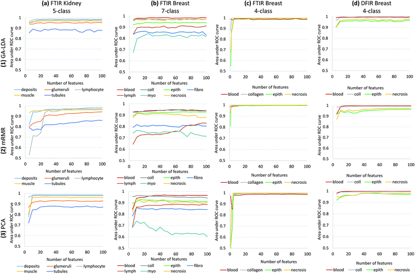
We compare the performance of three feature selection and extraction algorithms by validating on multiple tissue types and pathology-relevant classes (Fig. 6). We then provide measurements of the computational performance in order to justify our GPU-based implementation. Finally, we discuss practical implementation issues, including advice on parameter selection for various domain-specific goals.

Fig. 6 GA-LDA, PCA and mRMR performance is compared using validation results of (a) FTIR imaged kidney AMS701, (b) FTIR imaged breast TMA BRC961-BR1001 and (c) FTIR imaged breast tissue AMS802 (d) DFIR imaged breast tissue AMS802. Area under ROC curve for each class versus number of features selected by GA-LDA, mRMR or extracted by PCA are plotted. Our results suggest that GA-LDA significantly improves performance for complex data containing large numbers of classes. While GA-LDA exhibits similar performance to PCA for DFIR images, GA-LDA can be used for discrete-frequency imaging, thereby allowing users to take advantage of the main benefit of DFIR imaging systems.

3.1 Feature extraction and classifier performance

Results of feature selection and classification for GA-LDA, mRMR and PCA are shown in Fig. 6 for histological data sets including kidney and several breast cancer arrays. Comparison is based on the area under the receiver operating characteristic (ROC) curve for each class as a function of the number of features n. Note that feature selection is optimized for joint classification, which is why there is a visible difference in performance for the same class in different classifiers. For example, the necrosis class in our 4-class histology classifier exhibits better performance than in the 7-class example due to interference with the additional 3 classes (fibroblasts, lymphocytes, and myofibroblasts) (Fig. 6b and c). For small numbers of classes, GA-LDA performs comparably to existing methods such as PCA and mRMR (Fig. 6b). As additional classes are added, GA-LDA shows significant performance gain (Fig. 6a and b) compared to mRMR and PCA. In addition, GA-LDA allows the selected features to be utilized for DFIR imaging with comparable performance (Fig. 6d).

Training was performed in two steps: (1) feature selection/extraction using PCA, mRMR, and GA-LDA and (2) training of a random forest classifier. In order to test performance for varying parameters, different classifiers were created by varying numbers of features. There was no overlap between training and validation arrays. For breast histology, training was performed on a 101-core breast array (BR-1003, US Biomax) containing samples from 40 tumor biopsies of various types (hyperplasia, atypical hyperplasia, ductal carcinoma, and lobular carcinoma) and 7 normal biopsies. For kidney histology, training was performed on a 100-core kidney cortex array (AMS701, AMBbio).

The 5-class kidney is validated on independent cores from TMA AMS701 and validation results for 5-class kidney classifier shows that GA-LDA can achieve a high level of accuracy for even small numbers of features (Fig. 6a). Also, 7-class breast histology model was validated using two independent arrays (BRC961 and BR1001, US Biomax) containing a total of 196 cores from 100 different patients which were imaged using FTIR microscopy. This model shows the clear effectiveness of GA-LDA for selecting features that are compatible with a larger number of classes (Fig. 6). Validation on FTIR images of two types of tissues 5-class kidney and 7-class breast shows that GA-LDA can achieve a high level of accuracy for even small numbers of features for more number of classes as well (Fig. 6a and b). This model is generally superior to PCA, likely due to the use of a supervised training set. This implies that linear separability measured using Fisher's ratio provides a better overall optimization than feature variance. While there is significant use of the PCA approach for classification assuming it is more informative, this example illustrates nicely that complex signatures may be more robustly classified by use of discrete features. While the use of discrete features for rapid classification is more than a decade old,²⁶ the impetus for using discrete features was limited to speeding up post-acquisition processing. With faster computers and greater availability of storage, use of discrete features was not critical. Combined with the availability of DFIR imaging, however, the opportunity now exists to obtain more accurate classifications faster. This is particularly true for unusually complex chemical signatures, such as the differentiation of fibroblasts and myofibroblasts, as well as structures such as lymphocytes that are below the diffraction limit for IR. Finally, note that GA-LDA provides another advantage over PCA: the ability to translate features for use in DFIR imaging.

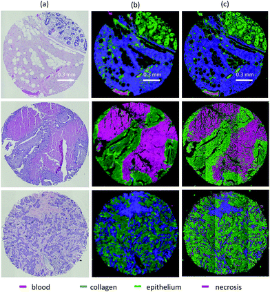
We test translation of GA-LDA features to DFIR using a 4-class model by validating on a 100-core (50 patient) array (AMS802, AMSbio). To demonstrate the methodology proposed here, instead of a comprehensive histologic analysis, we focused on testing of a 4-class model containing the most cancer-relevant cell types (epithelium, collagen, blood, and necrosis). The entire available spectrum (900–1800 cm⁻¹) was imaged to create a database of bands that would be compatible with any features selected or extracted using mRMR, PCA, and GA-LDA. Performance in both the FTIR and DFIR images are shown (Fig. 6c and d). Classification of both FTIR and DFIR imaged tissue cores using only 20 features selected from FTIR imaged data is shown in (Fig. 3).

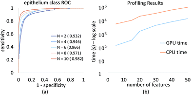
We demonstrate convergence of classifier performance for epithelium, which is the most important class for initial cancer diagnosis. The ROC curve (Fig. 7a) is shown for several feature selection values, and can be readily computed for large numbers of features on a desktop system. This allows a researcher or clinician to select the desired number of features to optimize for specificity, sensitivity, and image acquisition time.

Fig. 7 GA-LDA performance as a function of the number of selected features. (a) ROC curves for epithelium classification on DFIR breast images (AMS802) with different numbers of features. Area under ROC curve is mentioned in the legend corresponding to number of features used for the ROC plot. This plot shows how the ROC curve improves with the number of selected features. (b) Timing results are also shown for a traditional CPU and GPU implementation, demonstrating a 1–2 order of magnitude speedup on input data composed of 156k samples and 1626 bands for four different classes.

3.2 Computational performance

Profiling results also demonstrate the improvement in processing time using our GPU-based approach (Fig. 7b). This plot is in logarithmic scale of time in seconds, it shows that with GPU implementation of GA-LDA algorithm, we have achieved significant speed up in GA-LDA feature selection algorithm. This makes it faster with total population evaluation time required as minimum as evaluation time required for each genome. This speed-up depends on various parameters such as feature matrix size (S × B), population size (P) and number of features to be selected (N). The use of graphics hardware makes complex optimization problems more accessible to laboratories using traditional workstations and no programming experience.

3.3 Discussion

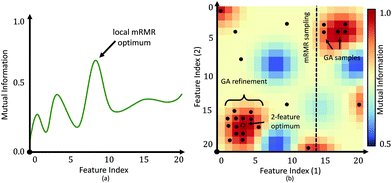
The main benefit of our GPU-based implementation is the fast calculation of AUC plots as a function of features (Fig. 6). This allows a domain expert to readily evaluate the number of features necessary to achieve the desired performance. Alternatively, a user can predict the accuracy that can be achieved within a specified time-frame, expressed in terms of the number of bands that can be collected.

While the proposed GA-LDA approach performs significantly better for larger numbers of classes, it also provides additional benefits when considering clinical translation of infrared spectroscopic imaging. Unlike feature extraction algorithms, such as PCA, GA-LDA features are compatible with DFIR instruments. GA-LDA algorithm also overcomes problem of getting trapped in local spectral region like mRMR as described in Fig. 4. In this figure, dotted line of mRMR sampling is a limited features space for second feature selection with mRMR after selection of first feature which is point on horizontal axis. This means mRMR algorithm cannot explore feature space beyond constrained region, whereas GA-LDA explores other regions in the feature space by introducing mutation in genomes. We also address execution time, which is the primary bottlneck for GA optimization, by providing a GPU-based implementation that can be run on inexpensive workstations available to both clinical and research laboratories.

We note that the proposed framework can be readily extended to manifold learning inspired fitness functions that may be more suitable when the class-conditional data are multi-modal or non-Gaussian. For instance, Local Fisher's ratio, which incorporates locality constraints in the Fisher's ratio through an affinity matrix⁴¹ ensure that multi-modal distributions remain multi-modal in the lower dimensional subspace and in the resulting set of selected features. In future work, we will consider this to overcome multi-modality in data set introduced by variations in tissue preparation and imaging environment.

4. Conclusion

Recent developments in mid-IR spectroscopic imaging are very promising, especially the potential of laser-based instrumentation to make it clinically applicable. FTIR imaging technology has been widely tested and it proved to demonstrate the concept of label free histopathology but has suffered from long acquisition times. The recent emergence of DFIR imaging has advantages like short imaging time, smaller pixel size, and hence more clinical applicability. Several different groups have achieved good results with DFIR technology^42,43 to demonstrate this potential but the question of choosing optical frequencies to scan remains an open question. Our results shows that spectral features selected from FTIR imaging data can satisfy several key needs – dimension reduction for FTIR imaging data and reducing imaging time and image size. Our study further indicates that with only these bands selected by GA-LDA we can achieve classification results equivalent to classification results with entire mid-IR spectrum. Fig. 7 shows, further, that the attempt to DFIR translation from FTIR data may actually result in improved classification. Thus, for complicated classification, a focus on extracting the maximum information content in an optimal manner can lead to improved protocols in all critical parameters – time for imaging, classification accuracy, ease of data handling and complexity of instruments.

In addition, feature selection makes DFIR imaging more practical if the desired classes are known a priori. This is particularly useful in a clinical environment, where there is a benefit to high-throughput screening of known diseases.

Finally, the proposed GPU-based implementation makes genetic algorithms far more practical to analytical scientists, since inexpensive hardware can be used to leverage a large computational benefit. The highly data-parallel nature of this problem allows full characterization of classifier performance across a large range of features, allowing biomedical researchers to carefully optimize for classification accuracy and imaging time. Together, the methods and results of this study propel analytical methods based on DFIR imaging forward to facilitate routine use of IR imaging for histopathology.

Conflicts of interest

There are no conflicts to declare.

Acknowledgements

This work was funded in part by the National Library of Medicine #4 R00 LM011390-02 (DM), National Institutes of Diabetes and Digestive and Kidney Diseases #1 R21 DK103066-01A1 (MJW), The National Institute for Biomedical Imaging and Bioengineering grant #R01 EB009745 (RB), the Cancer Prevention and Research Institute of Texas (CPRIT) #RR140013 (DM), and Agilent Technologies University Relations #3938 (DM), and The Agilent Thought Leader award (RB).

References

1. B. E. Bejnordi, G. Litjens, N. Timofeeva, I. Otte-Höller, A. Homeyer, N. Karssemeijer and J. A. van der Laak, IEEE Trans. Med. Imag., 2016, 35, 404–415.
2. C. Petibois and G. Deleris, Trends Biotechnol., 2006, 24, 455–462.
3. D. C. Fernandez, R. Bhargava, S. M. Hewitt and I. W. Levin, Nat. Biotechnol., 2005, 23, 469–474.
4. M. Pilling and P. Gardner, Chem. Soc. Rev., 2016, 45, 1935–1957.
5. O. Old, G. Lloyd, J. Nallala, M. Isabelle, L. Almond, N. Shepherd, C. Kendall, A. Shore, H. Barr and N. Stone, Analyst, 2017, 142, 1227–1234.
6. D. M. Mayerich, M. Walsh, A. Kadjacsy-Balla, S. Mittal and R. Bhargava, Proc. SPIE-Int. Soc. Opt. Eng, 2014, 904107.
7. A. Benard, C. Desmedt, M. Smolina, P. Szternfeld, M. Verdonck, G. Rouas, N. Kheddoumi, F. Rothé, D. Larsimont and C. Sotiriou, et al. , Analyst, 2014, 139, 1044–1056.
8. N. S. Ozek, S. Tuna, A. E. Erson-Bensan and F. Severcan, Analyst, 2010, 135, 3094–3102.
9. M. J. Walsh, M. N. Singh, H. M. Pollock, L. J. Cooper, M. J. German, H. F. Stringfellow, N. J. Fullwood, E. Paraskevaidis, P. L. Martin-Hirsch and F. L. Martin, Biochem. Biophys. Res. Commun., 2007, 352, 213–219.
10. A. Travo, O. Piot, R. Wolthuis, C. Gobinet, M. Manfait, J. Bara, M.-E. Forgue-Lafitte and P. Jeannesson, Histopathology, 2010, 56, 921–931.
11. M. Diem, L. Chiriboga and H. Yee, Biopolymers, 2000, 57, 282–290.
12. F. Großerueschkamp, A. Kallenbach-Thieltges, T. Behrens, T. Brüning, M. Altmayer, G. Stamatis, D. Theegarten and K. Gerwert, Analyst, 2015, 140, 2114–2120.
13. E. Gazi, M. Baker, J. Dwyer, N. P. Lockyer, P. Gardner, J. H. Shanks, R. S. Reeve, C. A. Hart, N. W. Clarke and M. D. Brown, Eur. Urol., 2006, 50, 750–761.
14. M. J. Baker, E. Gazi, M. D. Brown, J. H. Shanks, P. Gardner and N. W. Clarke, Br. J. Cancer, 2008, 99, 1859–1866.
15. P. Bassan, A. Sachdeva, J. H. Shanks, M. D. Brown, N. W. Clarke and P. Gardner, Proc. SPIE, 2014, 90410D–90416D.
16. R. Bhargava, Appl. Spectrosc., 2012, 66, 1091–1120.
17. P. Bassan, M. J. Weida, J. Rowlette and P. Gardner, Analyst, 2014, 139, 3856–3859.
18. J.-N. Liu, M. V. Schulmerich, R. Bhargava and B. T. Cunningham, Opt. Express, 2011, 19, 24182–24197.
19. M. Otto, Chemometrics: statistics and computer application in analytical chemistry, John Wiley & Sons, 2016.
20. M. Nie, Z. Liu, X. He, Q. Qiu, Y. Zhang and J. Chang, Appl. Opt., 2017, 56, 2476–2482.
21. Z. Movasaghi, S. Rehman and D. I. ur Rehman, Appl. Spectrosc. Rev., 2008, 43, 134–179.
22. K. Gajjar, J. Trevisan, G. Owens, P. J. Keating, N. J. Wood, H. F. Stringfellow, P. L. Martin-Hirsch and F. L. Martin, Analyst, 2013, 138, 3917–3926.
23. M. J. Baker, J. Trevisan, P. Bassan, R. Bhargava, H. J. Butler, K. M. Dorling, P. R. Fielden, S. W. Fogarty, N. J. Fullwood and K. A. Heys, et al. , Nat. Protoc., 2014, 9, 1771–1791.
24. D. Mayerich, M. J. Walsh, A. Kadjacsy-Balla, P. S. Ray, S. M. Hewitt and R. Bhargava, Technology, 2015, 3, 27–31.
25. J. T. Kwak, R. Reddy, S. Sinha and R. Bhargava, Anal. Chem., 2011, 84, 1063–1069.
26. R. Bhargava, D. C. Fernandez, S. M. Hewitt and I. W. Levin, Biochim. Biophys. Acta Biomembr., 2006, 1758, 830–845.
27. M. J. Pilling, A. Henderson and P. Gardner, Anal. Chem., 2017, 89, 7348–7355.
28. M. R. Kole, R. K. Reddy, M. V. Schulmerich, M. K. Gelber and R. Bhargava, Anal. Chem., 2012, 84, 10366–10372.
29. Z. M. Hira and D. F. Gillies, Adv. Bioinf., 2015, 2015 , 198363.
30. A. Zwielly, S. Mordechai, I. Sinielnikov, A. Salman, E. Bogomolny and S. Argov, Med. Phys., 2010, 37, 1047–1055.
31. J. Frost, L. Ludeman, K. Hillaby, R. Gornall, G. Lloyd, C. Kendall, A. C. Shore and N. Stone, Anal. Methods, 2016, 8, 8452–8460.
32. C. Krafft, L. Shapoval, S. B. Sobottka, K. D. Geiger, G. Schackert and R. Salzer, Biochim. Biophys. Acta Biomembr., 2006, 1758, 883–891.
33. N. Bergner, B. F. Romeike, R. Reichart, R. Kalff, C. Krafft and J. Popp, Analyst, 2013, 138, 3983–3990.
34. J. T. Kwak, S. M. Hewitt, S. Sinha and R. Bhargava, BMC Cancer, 2011, 11, 62.
35. R. Mankar, V. Verma, M. Walsh, C. Bueso-Ramos and D. Mayerich, Microsc. Microanal., 2016, 22, 1008.
36. L. Breiman, Mach. Learn., 2001, 45, 5–32.
37. H. Peng, F. Long and C. Ding, IEEE Trans. Pattern Anal. Mach. Intell., 2005, 27, 1226–1238.
38. D. E. Goldberg and K. Deb, Foundations of genetic algorithms, 1991, vol. 1, pp. 69–93.
39. M. Cui, S. Prasad, M. Mahrooghy, L. M. Bruce and J. Aanstoos, Geoscience and Remote Sensing Symposium (IGARSS), 2011 IEEE International, 2011, pp. 2373–2376.
40. M. Cui, S. Prasad, W. Li and L. M. Bruce, IEEE J. Sel. Topics Appl. Earth Observ. Remote Sens., 2013, 6, 1688–1697.
41. M. Sugiyama, J. Mach. Learn. Res., 2007, 8, 1027–1061.
42. N. Kröger, A. Egl, M. Engel, N. Gretz, K. Haase, I. Herpich, B. Kränzlin, S. Neudecker, A. Pucci and A. Schönhals, et al. , J. Biomed. Opt., 2014, 19, 111607–111607.
43. C. Hughes, G. Clemens, B. Bird, T. Dawson, K. M. Ashton, M. D. Jenkinson, A. Brodbelt, M. Weida, E. Fotheringham and M. Barre, et al. , Sci. Rep., 2016, 6 , 20173.

---