
 Open Access Article
 This Open Access Article is licensed under a
 Creative Commons Attribution 3.0 Unported Licence
Seasonal and latitudinal variability in the atmospheric concentrations of cyclic volatile methyl siloxanes in the Northern Hemisphere†
Frank
Wania
 ab,
Nicholas A.
Warner‡
c,
Michael S.
McLachlan
d,
Jeremy
Durham
e,
Merete
Miøen
c,
Ying Duan
Lei
ab and
Shihe
Xu§
*e
ab,
Nicholas A.
Warner‡
c,
Michael S.
McLachlan
d,
Jeremy
Durham
e,
Merete
Miøen
c,
Ying Duan
Lei
ab and
Shihe
Xu§
*e
aDepartment of Physical and Environmental Sciences, University of Toronto Scarborough, 1265 Military Trail, Toronto, Ontario M1C 1A4, Canada
bWECC Wania Environmental Chemists Corp., Toronto, Ontario, Canada
cNorwegian Institute for Air Research, Fram Centre, Tromsø, NO-9296, Norway
dDepartment of Environmental Science, Stockholm University, Stockholm, SE-106 91, Sweden
eToxicology and Environmental Research and Consulting, Dow Chemical Company, 1803 Building, Washington Street, Midland, MI 48674, USA. E-mail: shihe.xu@TECLMichigan.com
First published on 24th February 2023
Abstract
Field data from two latitudinal transects in Europe and Canada were gathered to better characterize the atmospheric fate of three cyclic methylsiloxanes (cVMSs), i.e., octamethyl-cyclotetrasiloxane (D4), decamethylcyclopentasiloxane (D5) and dodecamethylcyclohexasiloxane (D6). During a year-long, seasonally resolved outdoor air sampling campaign, passive samplers with an ultra-clean sorbent were deployed at 15 sampling sites covering latitudes ranging from the source regions (43.7–50.7 °N) to the Arctic (79–82.5 °N). For each site, one of two passive samplers and one of two field blanks were separately extracted and analyzed for the cVMSs at two different laboratories using gas-chromatography-mass spectrometry. Whereas the use of a particular batch of sorbent and the applied cleaning procedure to a large extent controlled the levels of cVMS in field blanks, and therefore also the method detection and quantification limits, minor site-specific differences in field blank contamination were apparent. Excellent agreement between duplicates was obtained, with 95% of the concentrations reported by the two laboratories falling within a factor of 1.6 of each other. Nearly all data show a monotonic relationship between the concentration and distance from the major source regions. Concentrations in source regions were comparatively constant throughout the year, while the concentration gradient towards remote regions became steeper during summer when removal via OH radicals is at its maximum. Concentrations of the different cVMS oligomers were highly correlated within a given transect. Changes in relative abundance of cVMS oligomers along the transect were in agreement with relative atmospheric degradation rates via OH radicals.
Environmental significanceCyclic volatile methylsiloxanes (cVMSs) are a class of environmental contaminants that are globally dispersed in the atmosphere. Atmospheric dispersion and reaction with OH radicals are known to be important processes governing their atmospheric fate, but some researchers have suggested that atmospheric deposition is also significant. Our work shows decreasing concentrations with increasing distance from the source regions, indicating that atmospheric loss processes are important. Both the seasonal variability of the concentration gradients and the differences in the concentration gradients between cVMS oligomers are consistent with phototransformation being an important fate process. Finally, the quality assured dataset provides an excellent basis for model-based experiments to explore the relevance of different fate processes. |
Introduction
Cyclic volatile methylsiloxanes (cVMSs) are a class of environmental contaminants under scrutiny due to their high production volume, release potential (due to their open uses and volatility), and potential for bioaccumulation in some aquatic systems to which they have been released.1,2 It is also well established from measurements in the remote atmosphere3 that cVMSs are globally dispersed. Although the bulk of the results, as compiled by McLachlan,4 suggest that cVMSs do not undergo atmospheric deposition in notable amounts, some researchers have suggested otherwise.5 Resolving this question is key to establishing whether cVMSs possess the potential for long-range transport in the sense of the Stockholm Convention.Better knowledge of the spatial and seasonal variability of atmospheric concentrations of cVMS on both regional and global scales could be useful in answering this question. Is the observed spatial and seasonal variability in the absolute concentrations and the relative abundance of cVMS oligomers attributable solely to reactive loss with the photo-oxidant OH6–10 or does atmospheric deposition or another atmospheric loss process11–14 need to be invoked? A model for which reaction with OH radicals was the dominant loss process succeeded in describing the temporal variability of D5 concentrations on a daily scale over 5 months at a regional background site in Scandinavia15 and on a ∼3-day scale over 46 days at a remote site in Svalbard.3 However, an assessment of this question on the basis of spatial variability in concentration and relative abundance of different cVMSs has yet to be undertaken.
Over the past decade, a substantial number of studies have reported on the concentration of cVMS in the atmosphere. While a compilation of existing data16 gives some indication of the spatial variability of cVMSs in the global atmosphere, the picture is complicated by (i) the question of the comparability of different sampling and analytical techniques, (ii) a strong bias in the sampled sites towards either source regions (mostly urban areas17,18) or remote regions (polar areas3) and (iii) occasionally a suspicion of break-through losses and/or blank contamination.
In principle, passive air sampler (PAS) networks are ideally suited to record the spatial variability of semi-volatile organic compounds on large spatial scales.19,20 This has been attempted for cVMSs with the sorbent impregnated polyurethane foam (SIP)-PAS on urban,21 regional,22 continental23 and global24 scales. Relative compositions of cVMS oligomers that deviate markedly from what is known about relative emission rates and concentration variability that is not always consistent with proximity to cVMS sources can cause skepticism about the reliability of the results from these studies. This may be related to the limited sorption capacity of the SIP for volatile compounds, which can mean that the sampler does not accumulate linearly over the deployment period, leading to difficulty in interpreting the results.20 A second explanation could be design features and quality control protocols that do not reliably prevent sample contamination, which is a major concern with cVMS analysis.25,26 The procedure for preparing SIPs by coating foam disks with ground XAD-powder is highly susceptible to sorbent contamination. Furthermore, a methylsiloxane-based silicone surfactant may be used as a processing aid in PUF manufacturing,27 and the polymeric siloxane residuals are not readily removed by washing. When PUF is deployed in the environment, cVMSs may be formed from such siloxane residuals.
Another PAS based on just XAD28 has been used to study cVMSs.17 It contains 50 times more XAD than the SIP-PAS20 and has been shown to linearly accumulate cVMS over 3-month deployment periods.17 During sample preparation the XAD is transferred directly into a mesh cylinder, a procedure with low risk of sorbent contamination. Also, the sampler contains no PUF. Consequently, this sampler should be better suited for monitoring cVMSs. However, detection limits previously achieved with this sampler17 are clearly insufficient for measurements outside of urban source regions.
In this study, we set out to use the XAD-based PAS to record the spatial and seasonal variability of cVMS concentrations in the atmosphere with a focus on the gradients between source regions in mid-latitudes and remote polar regions of the Northern Hemisphere. To increase the likelihood of generating useful data, we undertook a dedicated effort to lower detection limits by reducing blank contamination to the largest extent possible. To be able to understand the quality of the data generated, we included an extensive quality control scheme involving pairing each exposed sample with a field blank, duplication of sampling, and independent analysis of the duplicates in two laboratories.
Materials and methods
Air sampling
Ground-level outdoor air was sampled at 15 sites (Fig. 1) with PASs using a styrene-divinylbenzene copolymeric resin as a sorbent. The PAS, described previously,28 consists of a stainless-steel mesh cylinder (20 cm long and 2 cm diameter) that is filled with ∼20 g of sorbent (total mass of resin is recorded for each individual sampler) and closed with two aluminum crimping caps at either end. Each mesh cylinder is stored and transported in its own shipping container. During deployment the mesh cylinder is hung in a cylindrical stainless-steel housing that provides protection from precipitation, wind and sunlight. At sites north of the tree line that are more likely to experience high wind conditions, a modified housing was employed.29 The sampler housing was attached at a height of approximately 1.5 m above ground to a tree or an existing structure at the sampling site using metal hose clamps.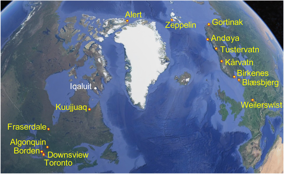 | ||
| Fig. 1 Map of the Northern Atlantic showing the passive air sampling locations along the Canadian (left) and European (right) transect. The site at Iqaluit had to be abandoned due to logistical difficulties. | ||
The sampling sites (coordinates given in Table S1†) were arranged along two south-to-north transects in Canada and Europe, ranging in latitude from 40 to 85 °N. The Canadian transect included seven sites and ranged from a site in downtown Toronto to Alert, Nunavut on Ellesmere Island in the Canadian Arctic Archipelago. Based on the expected concentration gradient, the distances between sampling sites at the southern end of the transect were much shorter than in the far north. The European transect consisted of eight sites ranging from Germany to Ny Ålesund, Svalbard in the European Arctic. As the concentration gradient was expected to be more gradual, sites along the European transect were more evenly spaced. The measurement of changes in the cVMS concentrations along latitudinal transects does not imply that we assume atmospheric transport to occur in a direct northerly direction between the sites of a continental transect. However, the complex patterns of atmospheric mixing on a hemispheric scale are expected to lead to declines in the seasonally averaged concentrations of cVMSs from source regions at mid-latitudes to remote regions at high latitudes that are controlled by atmospheric loss processes. Courier companies and the Canadian postal service were used to ship the samplers to and from the sampling sites, where local contacts performed the sampling following detailed instructions (see the Appendix in the ESI†).
Air was sampled for four sequential ∼3-month periods starting in November 2018. The exact time and total length of each deployment are given in Table S1.† Each deployment at all sites was duplicated and each exposed sampler was paired with a field blank (see below for details). For deployment, two resin-filled mesh tubes were taken out of the shipping tubes with a hook on the cap of the sampler housing (i.e., without the need to touch them) and hung in a single pre-cleaned sampler housing in the field. It has been previously shown that the rate of uptake in the sampler sorbent is not affected by the number of mesh cylinders placed within a housing.30 One exposed sampler and one field blank from each deployment were shipped for analysis to the Dow chemical company (Dow) in Midland, MI, USA and to the Norwegian Institute for Air Research (NILU) in Tromsø, Norway. The samplers were stored under cold conditions prior to laboratory processing.
Extraction and analysis
Standards and solvents used are described in Text S1 in the ESI.† For extraction, exposed mesh cylinders and field blanks were taken out of their shipping tubes in a clean cabinet and the sorbent from each mesh cylinder was emptied into a pre-cleaned and pre-weighed clear glass bottle. 60 ± 0.2 mL of hexane containing internal standards (ca. 3 ng g−1 sorbent) was added into the glass bottle containing the sorbent, which was closed with a pre-cleaned Teflon-lined cap and agitated on a vortex mixer for an hour. Approximately 4 mL of the hexane extract was transferred from the glass bottle to a pre-cleaned and baked (at 450 °C) 4 mL glass vial. An aliquot of the hexane extract was collected (ca. 1 mL into a vial without an insert, or ca. 0.2 mL into a vial with an insert). The extract was analyzed on an Agilent 7890A gas chromatograph (GC) connected to an Agilent 5975C mass spectrometer using selected ion monitoring (SIM). Details of the instrumental method and operation conditions used by Dow are reported in Table S2,† while details of the method used by NILU are described elsewhere.31Quality assurance/quality control
Atmospheric monitoring of cVMS is well-known for its susceptibility to both analyte loss from, and contamination of, the sample during sample collection, processing, and analysis.25,26 When sampling in remote locations, the risk of contamination compromising the measurement increases because concentrations are low and transport of samples to and from the sampling site can be long and complex. Several measures were adopted to minimize and monitor contamination.Three aliquots (0.5 g each) of resin from each bottle received from the vendor were analyzed for background concentrations of cVMS before use. A limit of detection based on sorbent contamination was calculated from the average plus 3.18 times the standard deviation of the procedural blank-corrected concentration (see below). The acceptable threshold was ≤1.04 ng g−1 for D4, 2.64 ng g−1 for D5, and 0.73 ng g−1 for D6; otherwise, the sorbent from that bottle was not used. For the European transect, a new batch of resin was used for each of the four deployments. The samplers deployed at the three northernmost sampling sites along the Canadian transect during all four seasons were from the same batch of sorbent, which is the same batch that was used at the four southern sites during the winter deployment. The samplers for the spring, summer, and fall deployments at the four southern Canadian sites were separately prepared and shipped to Toronto.
Data processing
All quantified amounts were normalised to the mass of sorbent and are provided in units of ng per g of sorbent, because different samplers can vary slightly in the amount of sorbent. The amounts of D4, D5, and D6 in field blanks and exposed air samples were first corrected by subtracting the average amounts in the procedural blanks of the corresponding batch. The amount of a cVMS in each exposed sampler (mexposed in ng g−1 sorbent) was then blank corrected with its paired field blank (mfield blank in ng g−1 sorbent), i.e., with the field blank deployed at the same site and during the same period and analyzed in the same laboratory. Because the actual deployment times (t in days) varied from 80 to 110 days on the Canadian transect and from 65 to 113 days on the European transect (Table S1†), the amounts were further normalized to a 90-day deployment period. Thus, the blank-corrected amounts m are in units of ng g−1 sorbent (90 days). By eliminating the effect of varied sampling time, comparisons between deployment periods and sites are facilitated.Volumetric air concentrations C in units of ng m−3 can be obtained using:
Results
QA/QC results and concentration data
The amounts of cVMS in procedural blanks were generally similar for D4 and D5 (0.1–0.4 ng g−1 sorbent) and lower for D6 (0–0.07 ng g−1 sorbent) (Table S3†). The spike recovery varied from 98.5 to 107.8% with little difference among the three cVMSs (Table S4†). The amounts of D4, D5, and D6 in field blanks and exposed air samples are given in Tables S5 and S6.† The amount in a field blank when expressed as a percentage of the amount in the exposed sampler from the same deployment site and period is strongly variable between the different compounds, different sampling sites and the two different transects (Text S3 and Table S7†). This is further discussed below.The blank-corrected amounts in exposed samplers from the Canadian and European transects are presented in Tables S8 and S9,† respectively. These tables also indicate whether a reported sorbent concentration is above the method detection limit (MDL) and quantitation limit (MQL), defined as 3 and 10 times the standard deviation of field blanks belonging to a particular resin batch (further details are provided in Text S4 and Table S10†). 86% and 79% of the samples had concentrations above the MQL for D4 and D5, respectively, including all of the samples from the European transect (Table S11†). Levels of D6 fall below the limits much more frequently, with 38% above the MQL (Table S11†).
We explored the interlaboratory agreement in the blank corrected amounts by plotting the discrepancy in m as determined by Dow and NILU against their average for the data >MQL (Fig. S2†). Overall, agreement between the results from the two laboratories was excellent. The bias is −0.01, 0.03 and 0.04![[thin space (1/6-em)]](https://www.rsc.org/images/entities/char_2009.gif) log units while the limits of agreement are ±0.13, ±0.16 and ±0.17log units for D4, D5 and D6, respectively. The latter implies that 95% of the concentrations from the two laboratories differed by less than a factor of 1.6 (upper limit for D6), which indicates that the method precision (including sampling, analysis and between-laboratory reproducibility) is good. In addition, there is little indication of proportional bias, i.e., the extent of disagreement is generally not related to the measured concentration levels.
log units while the limits of agreement are ±0.13, ±0.16 and ±0.17log units for D4, D5 and D6, respectively. The latter implies that 95% of the concentrations from the two laboratories differed by less than a factor of 1.6 (upper limit for D6), which indicates that the method precision (including sampling, analysis and between-laboratory reproducibility) is good. In addition, there is little indication of proportional bias, i.e., the extent of disagreement is generally not related to the measured concentration levels.
Comparison with earlier measurements
To establish that the air concentrations determined by the PASs in this study are plausible, comparison with measurements previously reported for Toronto, Downsview, Fraserdale, Alert and Zeppelin was carried out. The concentrations in unit of ng m−3 are provided in Tables S12 and S13† for the Canadian and European transects, respectively. The comparison, which is described in detail in Text S5, suggests that levels in Toronto have declined by a factor of approximately 2 to 2.5 over the last decade. Levels of D4 and D5 measured at the Arctic endpoints of the two transects are similar to those reported previously for Zeppelin and Alert, but D6 levels tended to be lower than the values reported earlier.Concentration patterns with latitude
All blank-corrected amounts m are displayed as a function of latitude in Fig. 2. Data below the MQL are included (shaded symbols) as they provide information on the approximate upper limit of the concentration. Discrepancies between the data from the two laboratories (comparing squares and circles of the same color at the same latitude in Fig. 2) are small relative to the overall range of measured concentrations. Given the low bias between the data obtained by Dow and NILU, the detailed data analysis was pursued on the basis of the average of the values, i.e., the combination of data reported by the two laboratories.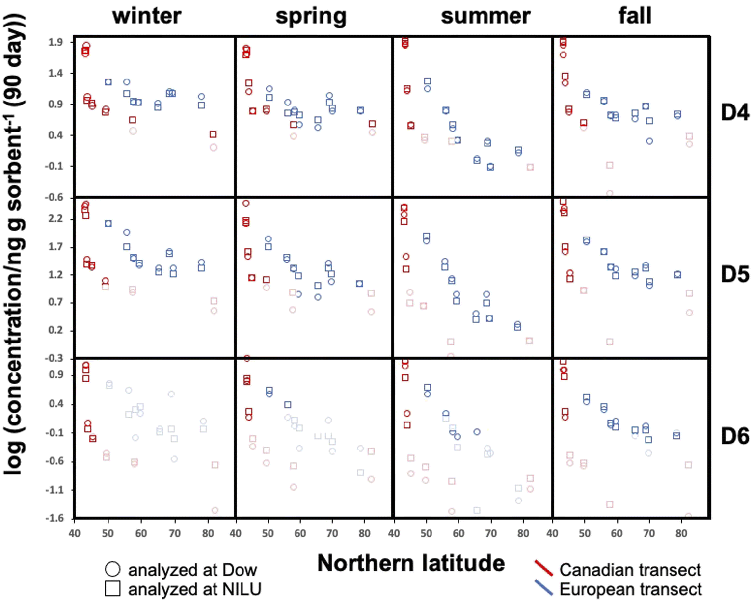 | ||
| Fig. 2 The decadic logarithm of the measured, blank-corrected concentrations in units of ng per sampler, normalized to 90 days, displayed as a function of the Northern latitude of the sampling site. The three rows of panels refer to the three different cVMSs and the four columns of panels represent the four seasonal deployments. Red and blue markers designate samplers deployed along the Canadian and European transect, respectively. The data reported by the two laboratories are depicted separately, using circles for data from Dow and squares for data from NILU. Data below the MQL are shaded. | ||
At the same latitude, concentrations along the European transects are always higher than those along the Canadian transect (blue markers are always above red markers in Fig. 2). The range of concentrations measured along the Canadian transect was greater compared to that along the European transect for all four seasons and all three compounds; maximum and minimum concentrations were always recorded in Toronto and Alert or Kuujjuaq within the Canadian Arctic, respectively. This can be partially attributed to the exclusion of large cities within the European transect.
Along both transects concentrations generally decline with increasing Northern latitude. The concentration decline with latitude is roughly log-linear along the European transect. While the Canadian transect shows an extremely steep decline at the four southernmost sampling sites (Toronto to Algonquin), the concentration differences between the three northernmost sites (Fraserdale to Alert) are fairly small despite the large latitudinal range. In some cases, the cVMS concentrations converge at high latitude, although Alert generally has lower levels than Zeppelin.
Seasonal concentration differences (comparing panels in different columns in Fig. 2) seem to be much less pronounced than the spatial differences. Most apparent is the occurrence of notably lower concentrations at higher latitudes for both transects during summer. As the concentrations at lower latitude show little seasonal change, steeper concentration declines with latitude are observed during summer. Seasonal concentration differences are discussed in more detail below.
Discussion
Analysis of the field blank results
This study was exceptional in terms of the number of field blank samplers deployed and analyzed (n = 120). This provided a wealth of information that allowed us to assess how the field blanks, and thus the MQL, were influenced by factors such as deployment period and site, the source and treatment of the XAD-resin, and the lab performing the analysis.Fig. 3 consolidates the data from the field blank analysis and allows for four key observations. First, differences in field blank levels caused by the analysis in two different laboratories are minor. This is apparent by comparing the left and right side of the plots in Fig. 3. This implies that the transport, storage, handling, and extraction of the samplers after deployment contribute little to the contamination of the field blanks. An important factor contributing to this result is the successful control of contamination sources in the laboratory, e.g., by performing the work in clean air cabinets. We further explored the agreement in the field blank levels determined by the two laboratories quantitatively by plotting the discrepancy in the field blank levels against their average (Text S6 and Fig. S3†). This plot shows that the bias between the two laboratories is small and that the discrepancy between them is independent of the field blank concentration.
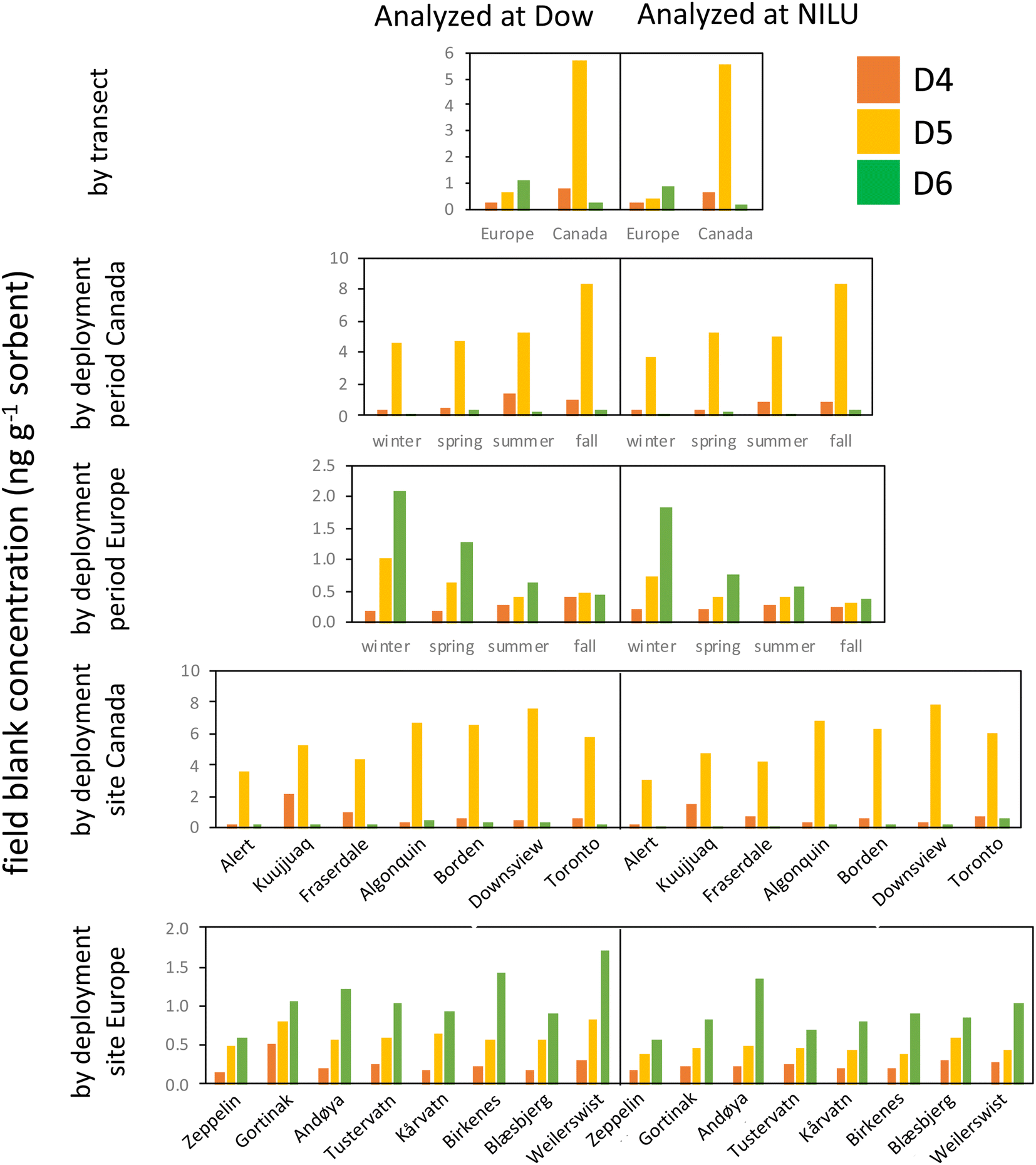 | ||
| Fig. 3 Field blank levels of the three cVMSs D4, D5, and D6 in passive samplers in units of ng g−1 sorbent, when grouped by transect (top row), deployment period (2nd and 3rd row) or deployment site (two bottom rows). Data on the left and right side were obtained by Dow and NILU, respectively. | ||
Second, levels in field blanks from the two transects are highly divergent (1st row in Fig. 3); the Canadian field blanks had much higher levels of D5 and D4, but lower levels of D6 compared to the European field blanks. Although the same resin was used for both transects, the resin was solvent washed prior to deployments in Europe, but not for deployments in Canada. It appears that the solvent cleaning step may have introduced additional D6, while reducing D4 and D5 residues on the resin.
Third, there are small, but notable differences in the field blank levels from the different deployment periods (2nd and 3rd row in Fig. 3). For example, in Europe, field blank levels of D6 decreased with every subsequent deployment (winter to spring to summer to fall), whereas the opposite was the case for D4 (although the latter was more pronounced in samplers analyzed at Dow than at NILU). The differences between deployments were attributed to the different batches of resin. Every batch had its own distinct cVMS signature. For example, the last batch of samplers prepared for the fall deployment at the four southern Canadian sites had unusually high D5 and D6 levels, but was relatively low in D4.
Fourth, the last two rows in Fig. 3 show that at a few sites field blanks were elevated (e.g., D4 at Kuujjuaq) even if the same batch of resin is used (Fig. S4†). This indicates that the conditions that are specific to a given sampling site, such as the specific transport route to and from the site, the storage of samplers on site or the specific deployment and retrieval procedure, may contribute to field blank levels. However, the remarkable consistency of the blank signature between the eight European sampling sites (especially when analyzed by NILU) indicates that these sources of field blank contamination are minor in most cases.
In summary, the use of a particular batch of resin appears to be of overarching importance in controlling the levels of cVMSs in PAS field blanks. Even if the same resin supplier and cleaning procedure is used, differences in field blank levels in samplers prepared at different times can be expected to occur. The large and consistent differences between samplers deployed in Canada and Europe suggest that the resin contamination with D4 and D5 did not originate during sampler preparation (e.g., the filling of the resin into mesh tubes), but rather was present in the resin from the outset and could be reduced by solvent cleaning. However, the higher background for D6 in the European samples suggests that solvent cleaning the resin also introduced D6. Future studies should, at a minimum, employ field blanks that are specific to each batch of prepared samplers. However, the differences observed in the field blanks at some sites using the same batch of sampler/resin suggest that field blank contamination can be site specific and deployment of site-specific field blanks, as done in the current study, is advisable.
Seasonal variability in the latitudinal gradients
To investigate the seasonal variability in the latitudinal profiles in detail, Fig. 4 plots the data >MQL from the four deployments in the same panel. This is done for each compound and the two transects, using the average of the duplicate samples. Whereas seasonal concentration differences in the source regions at the southern end of the respective transects are generally small, distinct differences in the seasonal profiles along the European transect are revealed in Fig. 4. The concentrations are highest in winter and lowest in summer, resulting in shallower and steeper declines with increasing latitude during those seasons. The gradients measured in spring and fall are similar and lie in between those of the two other seasons.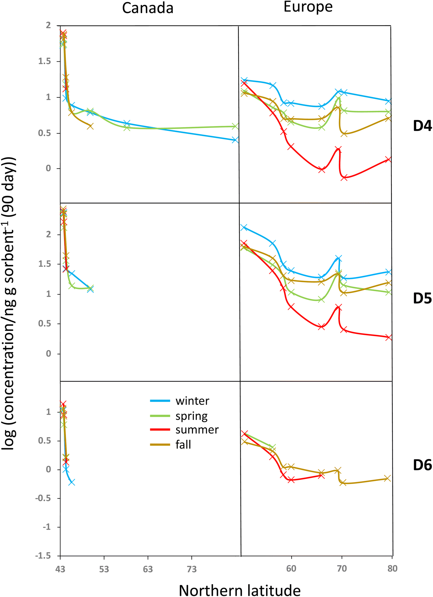 | ||
| Fig. 4 The decadic logarithm of the measured, blank-corrected concentrations above the MQL in units of ng per sampler, normalized to 90 days, displayed as a function of the Northern latitude of the sampling site. Colors designate samplers deployed during different seasons. The average of the concentrations measured by the two laboratories is shown by the symbols. The symbols are connected by a line to facilitate visualization. | ||
Temperature is not expected to have a sizeable effect on the atmospheric fate of cVMSs because partitioning of cVMS to atmospheric particles and liquid water is negligible, even at low temperatures.35 Variation in solar irradiation clearly has the most influence on seasonal variability of cVMS concentrations at higher latitudes, because a higher solar irradiance increases the concentration of photooxidants such as the hydroxyl radical. As oxidation by photooxidants is the major process known to remove cVMSs from the atmosphere,4 one could anticipate that seasonal differences in concentrations would be related to the seasonal variation in the day length. The average day length during the deployments followed the order of winter < fall < spring < summer. The seasonal variability in cVMS concentrations along the European transect is largely consistent with this.
For the Canadian transect there were insufficient data >MQL to allow assessment of seasonal variability. However, the gradients at the southern end of the Canadian transect were much steeper than the gradients at the southern end of the European transect. This was anticipated because this part of the Canadian transect transitioned in a short distance from the core of a heavily populated urban metropolis to a rural region with few large proximate upwind population centers while the European transect contained only rural or remote sampling sites and progressed away from a source region with a more gradual decline in population density.
Relationship between different cVMSs
Except at their Northern terminals, the relative composition of the cVMS oligomers differs slightly between Canada and Europe. In Canada, D4 and D6 contribute a relatively larger and smaller share, respectively, to the total cVMS than in Europe. This suggests that cVMS emissions in the two continents have slightly different compositions. The primary source of D4 emissions in the USA has been reported to be adhesives, while the primary source of D5 is personal care products.36Within a given transect, both D4 and D6 were highly correlated with D5, with r2 ranging from 0.88 to 0.98 (Fig. 5). This is in contrast to other studies, that observed no or weaker correlations. For example, a passive sampling study in Tibet found no correlation between D6 and D5 and a considerably weaker correlation between D4 and D5.22 In PASs deployed globally, a good correlation between D6 and D5 was observed (r2 = 0.79) but there was none between D4 and D5.24
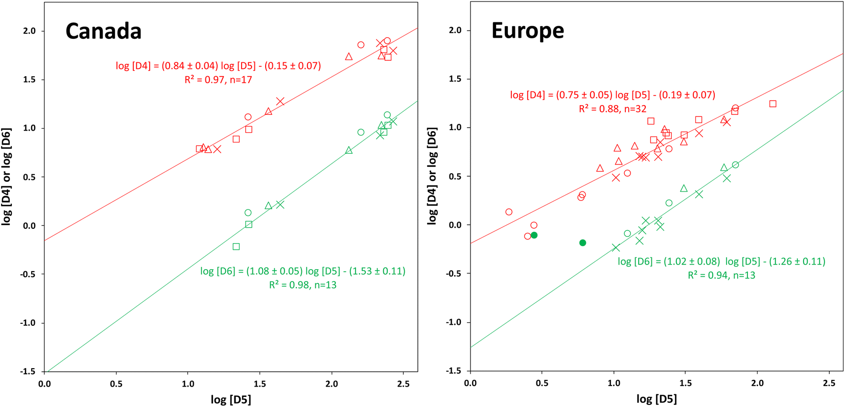 | ||
| Fig. 5 Correlation of the field-blank corrected concentrations in ng g−1 sorbent normalized to 90 days of D4 (red) and D6 (green) with D5, shown separately for the Canadian (left) and European (right) transects. The different seasons are designated with different marker styles, square: winter, triangle: spring, circle: summer, and cross: fall. Only data above the MQL are plotted. The two filled green circles were not included in the regression. | ||
The slopes of the plots of logD4 versus logD5 were 0.84 ± 0.04 for Canada and 0.75 ± 0.05 for Europe, i.e., as the concentration of D5 decreased, that of D4 decreased as well, but to a lesser extent. For logD6 on the other hand, slopes >1 were obtained (1.08 ± 0.05 for Canada and 1.02 ± 0.08 for Europe), indicating that the concentration of D6 decreased slightly more rapidly than the concentration of D5 in Canada. As noted above, cVMS concentrations at the southern (source) end of the transects were highest and similar for all seasons. This represents the right-hand end of the plots in Fig. 5. The decrease in concentration as one moves left on the plots reflects dilution and removal of cVMSs as they are transported away from the source region. We anticipate the decrease of D4 concentration to be slower than the decrease of D5 concentration because of the lower rate constant for photo-oxidation by OH radicals.6,8,9 For D6, the decrease in concentration is expected to be similar to,8 or faster9 than, that of D5 depending on which set of reaction rate constants is selected. Hence our observations align well with expectations.
Application of passive sampling for evaluating the atmospheric fate of cVMSs
This study shows that high quality data on atmospheric spatial variability of cVMSs can be obtained using passive sampling if extraordinary attention is paid to quality assurance. The large effort expended in this study resulted in a reduction in the average MQL of the method compared to the earlier study using the XAD-based PAS17 by a factor of 67 (D4), 33 (D5) and 118 (D6), largely as a result of a reduction in blank contamination. Nevertheless, the sampling campaign was only moderately successful, with quantification of D4, D5 and D6 being possible in 86%, 79% and 38% of the samples, respectively. This success was constrained by the MQL, which in turn was constrained by the blank levels. The dominant source of blank contamination in this study was the sorbent and its preparation. To further reduce the MQL, more attention should be paid to studying sorbent quality and contamination variability, and procedures to improve sorbent quality (i.e., solvent washing) should be developed.Furthermore, this study demonstrates the importance of employing extensive and comprehensive QA/QC programs. The blanks in this study were not only useful for identifying the factors constraining the MQL, but were essential for developing a strong method for determining the MQL and thereby quality assuring the dataset. The calculation of the MQL can benefit greatly from an understanding of the dominant source of variability in the blanks. In this study, we established that the variability could, in most cases, be attributed to the sorbent batch. In doing so we avoided adopting a more conservative definition of the MQL that would have needlessly resulted in fewer data passing the >MQL criterion.
In this report, we show that several observations from this study are qualitatively consistent with the current understanding of the fate of cVMSs in the atmosphere. A more quantitative evaluation would require assembling the functional relationship between the major variables influencing cVMS concentrations such as the distance from sources, wind speed, air temperature and sunlight duration, and integrating this relationship over the respective sampling period. We plan to address this challenge in future work by using a mathematical model of atmospheric circulation and chemistry to simulate cVMS concentrations at the sampling sites. Comparison of the model simulations with our observation will provide further insight into our ability to describe the long-range atmospheric transport of cVMSs.
Conflicts of interest
Shihe Xu was at the time of conducting this study and Jeremy Durham continues to be an employee of Dow Chemical Company, an organosilicon manufacturer.Acknowledgements
We acknowledge funding from Silicones Europe (CES) Project No. 02/444/S040/07/0269. We are grateful to the following people who helped with sampler deployment and/or site access in Canada: Kevin Rawlings, Melody Fraser, Andrew Platt (Dr Neil Trivett Global Atmosphere Watch Observatory, Alert), Lucassie Peter, Jason Carpenter (Arctic College, Iqaluit), Michael Kwan (Makivik Corp., Kuujjuaq), Andre LeClerc (Fraserdale), Kevin Kemmish (Algonquin Wildlife Research Station), Ralf Staebler (Borden) and Chubashini Shunthirasingham (Downsview), and in Europe: the Norwegian Polar Institute engineer team at Zeppelin Observatory, Tore Flatlands Berglen (Gortinak), Reidar Lyngra (Andøya), Are Bäcklund (Tustervatn), Dorothea Schultze (Kårvatn), Olav Lien (Birkenes), Stephan Bernberg (Blæsbjerg) and Barbara Schmitt (Weilerswist). Many thanks to Jessica Betz, Regan Streeter and Coreena Cheney for help in sampler preparation, shipping and analysis at Dow.References
- Y. Horii and K. Kannan, Main uses and environmental emissions of volatile methylsiloxanes, in Volatile Methylsiloxanes in the Environment. The Handbook of Environmental Chemistry, ed. V. Homem and N. Ratola, Springer, Cham, 2020, vol. 89, pp. 33–70 Search PubMed.
- S. Augusto, Bioconcentration, bioaccumulation, and biomagnification of volatile methylsiloxanes in biota, in Volatile Methylsiloxanes in the Environment. The Handbook of Environmental Chemistry, ed. V. Homem and N. Ratola, Springer, Cham, 2020, vol. 89, pp. 247–277 Search PubMed.
- I. S. Krogseth, A. Kierkegaard, M. S. McLachlan, K. Breivik, K. M. Hansen and M. Schlabach, Occurrence and seasonality of cyclic volatile methyl siloxanes in Arctic air, Environ. Sci. Technol., 2013, 47, 502–509 CrossRef CAS PubMed.
- M. S. McLachlan, Atmospheric fate of volatile methyl siloxanes, in Volatile Methylsiloxanes in the Environment. The Handbook of Environmental Chemistry, ed. V. Homem and N. Ratola, Springer, Cham, 2020, vol. 89, pp. 227–24 Search PubMed.
- J. Sanchís, A. Cabrerizo, C. Galbán-Malagón, D. Barceló, M. Farré and J. Dachs, Unexpected occurrence of volatile dimethylsiloxanes in Antarctic soils, vegetation, phytoplankton, and krill, Environ. Sci. Technol., 2015, 49, 4415–4424 CrossRef PubMed.
- R. Atkinson, Kinetics of the gas phase reactions of a series of organosilicon compounds with OH and NO3 radicals and O3 at 297.2 K, Environ. Sci. Technol., 1991, 25, 863–866 CrossRef CAS.
- R. Xiao, I. Zammit, Z. Wei, W.-P. Hu, M. MacLeod and R. Spinney, Kinetics and mechanism of the oxidation of cyclic methylsiloxanes by hydroxyl radical in the gas phase: an experimental and theoretical study, Environ. Sci. Technol., 2015, 49, 13322–13330 CrossRef CAS PubMed.
- A. Safron, M. Strandell, A. Kierkegaard and M. MacLeod, Rate constants and activation energies for gas-phase reactions of three cyclic volatile methyl siloxanes with the hydroxyl radical, Int. J. Chem. Kinetics, 2015, 47, 420–428 CrossRef CAS PubMed.
- J. Kim and S. Xu, Quantitative structure-reactivity relationships of hydroxyl radical rate constants for linear and cyclic volatile methylsiloxanes, Environ. Toxicol. Chem., 2017, 36, 3240–3245 CrossRef CAS PubMed.
- F. Bernard, D. K. Papanastasiou, V. C. Papadimitriou and J. B. Burkholder, Temperature dependent rate coefficients for the gas-phase reaction of the OH radical with linear (L2, L3) and cyclic (D3, D4) permethylsiloxanes, J. Phys. Chem. A, 2018, 122, 4252–4264 CrossRef CAS PubMed.
- J. Kim and S. Xu, Sorption and desorption kinetics and isotherms of volatile methylsiloxanes with atmospheric aerosols, Chemosphere, 2016, 144, 555–563 CrossRef CAS PubMed.
- J. G. Navea, S. Xu, C. O. Stanier, M. A. Young and V. H. Grassian, Effect of ozone and relative humidity on the heterogeneous uptake of octamethylcyclotetrasiloxane and decamethylcyclopentasiloxane on model mineral dust aerosol components, J. Phys. Chem. A, 2009, 113, 7030–7038 CrossRef CAS PubMed.
- J. G. Navea, S. Xu, C. O. Stanier, M. A. Young and V. H. Grassian, Heterogeneous uptake of octamethylcyclotetrasiloxane (D4) and decamethylcyclopentasiloxane (D5) onto mineral dust aerosol under variable RH conditions, Atmos. Environ., 2009, 43, 4060–4069 CrossRef CAS.
- J. G. Navea, M. A. Young, S. Xu, V. H. Grassian and C. O. Stanier, The atmospheric lifetimes and concentrations of cyclic methylsiloxanes octamethylcyclotetrasiloxane (D4) and decamethylcyclo-pentasiloxane (D5) and the influence of heterogeneous uptake, Atmos. Environ., 2011, 45, 3181–3191 CrossRef CAS.
- M. S. McLachlan, A. Kierkegaard, K. Hansen, R. Van Egmond, J. Christensen and C. Skjøth, Concentrations and fate of decamethylcyclopentasiloxane (D5) in the atmosphere, Environ. Sci. Technol., 2010, 44, 5365–5370 CrossRef CAS PubMed.
- S. Xu, N. Warner, P. Bohlin-Nizzetto, J. Durham and D. McNett, Long-range transport potential and atmospheric persistence of cyclic volatile methylsiloxanes based on global measurements, Chemosphere, 2019, 228, 460–468 CrossRef CAS PubMed.
- I. S. Krogseth, X. Zhang, Y. D. Lei, F. Wania and K. Breivik, Calibration and application of a passive air sampler (XAD-PAS) for volatile methylsiloxanes, Environ. Sci. Technol., 2013, 47, 4463–4470 CrossRef CAS PubMed.
- R. A. Yucuis, C. O. Stanier and K. C. Hornbuckle, Cyclic siloxanes in air, including identification of high levels in Chicago and distinct diurnal variation, Chemosphere, 2013, 92, 905–910 CrossRef CAS PubMed.
- L. Shen, F. Wania, Y. D. Lei, C. Teixeira, D. C. G. Muir and T. F. Bidleman, Atmospheric distribution and long-range transport behavior of organochlorine pesticides in North America, Environ. Sci. Technol., 2005, 39, 409–420 CrossRef CAS PubMed.
- F. Wania and C. Shunthirasingham, Passive air sampling for semivolatile organic compounds, Environ. Sci.: Processes Impacts, 2020, 22, 1925–2002 RSC.
- L. Ahrens, T. Harner and M. Shoeib, Temporal variations of cyclic and linear volatile methylsiloxanes in the atmosphere using passive samplers and high-volume air samplers, Environ. Sci. Technol., 2014, 48, 9374–9381 CrossRef CAS PubMed.
- X. Wang, J. Schuster, K. C. Jones and P. Gong, Occurrence and spatial distribution of neutral perfluoroalkyl substances and cyclic volatile methylsiloxanes in the atmosphere of the Tibetan Plateau, Atmos. Chem. Phys., 2018, 18, 8745–8755 CrossRef CAS.
- C. Rauert, T. Harner, J. K. Schuster, A. Eng, G. Fillmann, L. E. Castillo, O. Fentanes, M. Villa Ibarra, K. S. B. Miglioranza, I. Moreno Rivadeneira, K. Pozo and B. H. Aristizábal Zuluaga, Air monitoring of new and legacy POPs in the Group of Latin America and Caribbean (GRULAC) region, Environ. Pollut., 2018, 243, 1252–1262 CrossRef CAS PubMed.
- S. Genualdi, T. Harner, Y. Cheng, M. MacLeod, K. J. Hansen, R. van Egmond, M. Shoeib and S. Lee, Global distribution of linear and cyclic volatile methyl siloxanes in air, Environ. Sci. Technol., 2011, 45, 3349–3354 CrossRef CAS PubMed.
- V. Homem and N. Ratola, Analytical methods for volatile methylsiloxanes quantification: current trends and challenges, in Volatile Methylsiloxanes in the Environment. The Handbook of Environmental Chemistry, ed. V. Homem and N. Ratola, Springer, Cham, 2020, vol. 89, pp. 71–118 Search PubMed.
- R. Gerhards, R. M. Seston, G. E. Kozerski, D. A. McNett, T. Boehmer, J. A. Durham and S. Xu, Basic considerations to minimize bias in collection and analysis of volatile methyl siloxanes in environmental samples, Sci. Total Environ., 2022, 851(Part 2), 158275 CrossRef CAS PubMed.
- X. D. Zhang, C. W. Macosko, H. T. Davis, A. D. Nikolov and D. T. Wasan, Role of silicone surfactant in flexible polyurethane foam, J. Colloid Interface Sci., 1999, 215, 270–279 CrossRef CAS PubMed.
- F. Wania, L. Shen, Y. D. Lei, C. Teixeira and D. C. G. Muir, Development and calibration of a resin-based passive sampling system for persistent organic pollutants in the atmosphere, Environ. Sci. Technol., 2003, 37, 1352–1359 CrossRef CAS.
- P. Gong, X. Wang, X. Liu and F. Wania, Field calibration of XAD-based passive air sampler on the Tibetan Plateau: wind influence and configuration improvement, Environ. Sci. Technol., 2017, 51, 5642–5649 CrossRef CAS PubMed.
- X. Zhang, M. Hoang, Y. D. Lei and F. Wania, Exploring the role of the sampler housing in limiting uptake of semi-volatile organic compounds in passive air samplers, Environ. Sci.: Processes Impacts, 2015, 17, 2006–2012 RSC.
- N. Warner, V. Nikiforov, I. S. Krogseth, S. M. Bjørneby, A. Kierkegaard and P. Bohlin-Nizzetto, Reducing sampling artifacts in active air sampling methodology for remote monitoring and atmospheric fate assessment of cyclic volatile methylsiloxanes, Chemosphere, 2020, 255, 126967 CrossRef CAS PubMed.
- Y. Li and F. Wania, Partitioning between polyurethane foam and the gas phase: data compilation, uncertainty estimation and implications for air sampling, Environ. Sci.: Processes Impacts, 2021, 23, 723–734 RSC.
- X. Zhang, T. N. Brown, A. Ansari, B. Yeun, K. Kitaoka, A. Kondo, Y. D. Lei and F. Wania, Effect of wind on the chemical uptake kinetics of a passive air sampler, Environ. Sci. Technol., 2013, 47, 7868–7875 CrossRef CAS PubMed.
- I. Al Saify, Development of an Active and Passive Air Sampling Methodology for Atmospheric Monitoring of Cyclic Volatile Methyl Siloxanes and Chlorinated Paraffins, Master's thesis, Vrije Universiteit, Amsterdam, 2020 Search PubMed.
- S. Xu and F. Wania, Chemical fate, latitudinal distribution and long-range transport of cyclic volatile, methyl–siloxanes in the global environment: a modelling assessment, Chemosphere, 2013, 93, 835–843 CrossRef CAS PubMed.
- G. I. Gkatzelis, M. M. Coggon, B. C. McDonald, F. Peischl, K. C. Aikin, J. B. Gilman, M. Trainer and C. Warneke, Identifying volatile chemical product tracer compounds in U.S. cities, Environ. Sci. Technol., 2021, 55, 188–199 CrossRef CAS PubMed.
Footnotes |
| † Electronic supplementary information (ESI) available. See DOI: https://doi.org/10.1039/d2em00467d |
| ‡ Current affiliation: Thermo Fisher Scientific, Bremen, Germany. |
| § Current affiliation: Tridge Environmental Consulting, Midland, Michigan, 48642, USA. |
| This journal is © The Royal Society of Chemistry 2023 |