A robotic approach to polymerisation kinetics: a case study on copolymerisation parameter estimation

Abstract

Automation and high-throughput (HTP) experimentation are transforming chemistry, yet the high cost of robotic platforms limits accessibility. Pipetting robots such as the Opentrons OT-2 provide a cost-effective, open-source alternative, but their application to radical polymerisation in high throughput formats has been restricted by challenges such as deoxygenation at microlitre scale. Here, we establish a robust workflow for thermal radical polymerisation in a 48-well reactor using the OT-2, supported by custom 3D-printed components for automated NMR sample preparation. This system enables rapid and reproducible data generation while eliminating human bias from experimentation. We demonstrate its utility through the study of copolymerisation kinetics, where inconsistent methods, reporting, and model selection have created significant data gaps for predictive modelling. By combining robotic HTP experimentation with IUPAC-recommended evaluation methodology, we provide standardised datasets for predicting reactivity ratios of six monomer pairs: BMA-BA (r₁ = 2.22, r₂ = 0.37), BMA-St (r₁ = 0.58, r₂ = 0.73), St-BA (r₁ = 1.23, r₂ = 0.32), St-MMA (r₁ = 0.46, r₂ = 0.58), GMA-BA (r₁ = 1.77, r₂ = 0.24), and GMA-St (r₁ = 0.69, r₂ = 0.32). Each dataset can be generated and analysed within hours, offering a powerful automated platform for systematic polymerisation studies. This work establishes the OT-2 as a practical, accessible tool for accelerating polymer research and enabling data-driven chemical discovery.

---

Introduction

Classical high-throughput (HTP) experimentation and its modern counterpart, robotic laboratory experimentation, are rapidly transforming the way chemistry is conducted, and polymer science is no exception. Robotic platforms provide accuracy, reproducibility, and efficiency to synthetic workflows, offering a path to generate data at a scale and quality that manual experimentation cannot easily achieve. Various automation platforms have been applied over the years, such as the popular Chemspeed platform, which offers parallel synthesis and sample preparation for a wide range of chemistries and applications.¹ High-end platforms of this kind are, however, cost-intensive, posing a hurdle for many research laboratories. Pipetting robots have emerged as a cost-effective alternative. Originally developed for biochemical investigations – where parallelisation and standardised reagents handling are routine, such as in biological assays and PCR tests – these robots are increasingly being adopted by synthetic chemists. For example, a Hamilton MLSTARlet liquid handling robot has been used for the synthesis of a variety of homopolymers, copolymers, and polymer protein hybrids via thermal and/or photo RAFT polymerisation.² Similarly, a Biomek NX^P MC liquid handling robot has been used for the automated synthesis of multiblock star copolymers.³ The Opentrons OT-2 liquid handling robot is another emerging platform that offers flexibility and open-source code, and has already been used for the automated synthesis of libraries of complex multiblock copolymers,⁴ as well as libraries of block-copolymer-based hydrogels for biomedical applications.⁵

Reaction kinetics and synthetic polymer chemistry are inexorably intertwined. Since practically any polymer is the result of a cascade of reactions, typically involving at least initiation, propagation and termination, the structure of a polymer product is always defined by its underpinning kinetics and the associated rate coefficients.⁶ Thus, the study of polymerisation kinetics is more than a physical chemistry exercise. Rather, it is fundamental for the design of new polymers, and for rational design of materials. This is especially true in a research landscape that is becoming increasingly data-driven. Traditionally, many synthesis methods were developed on a strong kinetic foundation, but in reality, practitioners often do not need to worry about rate coefficients. For example, one does not need to know individual rate coefficients to perform reversible deactivation radical polymerisations such as reversible addition-fragmentation chain transfer (RAFT) polymerisation⁷ or atom transfer radical polymerisation (ATRP).⁸ Nonetheless, knowing these values is extremely useful, particularly when testing the boundaries of existing methods towards new synthetic goals, such as multiblock copolymers or ultra-high molecular weight polymers.^1,9

One particular area where precise knowledge of rate coefficients and their interdependency is of the highest importance is the design of statistical copolymers.¹⁰ Industrially, statistical copolymers are of very high relevance, and arguably the need to develop more sustainable materials that allow for circular use of feedstocks will only increase this demand.¹¹ The specific copolymerisation kinetics, more precisely the individual probabilities of monomers being added to a growing chain end, define the copolymer sequence, and thus directly the properties of the resulting polymer.¹² Moreover, if the individual probabilities are significantly different from each other, then the resulting copolymer composition (F) will not only be different from the comonomer feed (f), but also notably change during a polymerisation (called composition drift), increasing the inhomogeneity of a synthetic product.¹³ Decades of research have thus been dedicated to understanding the exact interplay of propagation reactions to reach understanding and precise macromolecular engineering tools. While complex kinetic models have been built and validated to help gain mechanistic insights into copolymerisation reactions, such as the implicit and the explicit penultimate model,¹⁴ most researchers until today rely on the terminal model of copolymerisation. This model assumes that growing chains will have a radical terminus stemming from monomer M₁ or monomer M₂ in the copolymerisation, which are the only effective factors governing the reactivity of the growing polymer chain.¹⁵ Both can add each other's monomers, thus yielding 4 individual propagation reactions that are associated with the rate coefficients k₁₁, k₁₂, k₂₁ and k₂₂. To simplify, one usually then considers the reactivity ratios r₁ and r₂, as defined in Fig. 1, part C to reduce the number of parameters. With these reactivity ratios, one can then determine the relationship of F and f as a function of monomer conversion via the so-called Mayo–Lewis equation.¹⁶ Especially on the background of synthesis of polymers with specific physical properties, precise control over the copolymer composition is mandatory, and hence good knowledge of the underpinning reactivity ratios.

Fig. 1 Overview of the HTP data generation workflow for reactivity ratio prediction in free-radical polymerisation. In part A, a Python script is executed to prepare microlitre scale reaction mixtures in a 48-well reactor, as well as the in situ preparation of NMR samples for initial screening (1). The reactor is then transferred to a heater-shaker for copolymerisation (2). The reactor is then returned to the automation platform for further sampling (3). Part B includes analysis, where all NMR samples are transferred to the NMR facility for characterisation and analysis (4 and 5). In part C, the program Contour is used to estimate reactivity ratios (r₁ and r₂) for binary monomer systems using the NLLS method.²⁸

As mentioned, more complex and more accurate models have been shown to be superior to the terminal model. For example, the terminal model generally fails to predict both the rate of polymerisation and the copolymer composition at the same time.¹⁷ The reason that the more complex models are, however, not widely used is that experimental data are largely lacking, and providing accurate data for the more complex models is a very time-consuming task, further requiring elaborate fitting procedures. Further, even for the terminal model, many different determination methods exist, and it is already difficult to find consensus for r₁ and r₂ for most monomer pairs (see SI for a selection of literature results for monomers studied in here). An IUPAC working party thus critically evaluated reactivity ratio determination methods and developed a general methodology for the fitting of copolymerisation data that should in future ensure a better understanding of the available data.¹⁸ A unified approach will remove inherent biases, identify experimental data of low accuracy and eventually allow to compare reactivity ratios across a larger array of monomers. Hopefully with this, machine learning (ML) will become more effective, and then allow for proper prediction of copolymerisations with a broad scope. Interesting advances have already been made for homopropagation rate coefficient prediction,¹⁹ and also for reactivity ratio predictions using ML, for which availability of quality data has been determined as the current limiting factor in prediction accuracy.²⁰

Against this background, copolymerisation kinetic studies serve as an ideal case study for demonstrating the power of automated approaches. Leibfarth and team have previously developed a somewhat related method,²¹ who utilised flow chemistry in an automated fashion to overcome the tediousness of generating numerous measurement samples by collecting NMR samples directly from the flow reactor, while comonomer composition could be automatically altered in subsequent iterations. However, even with this approach, only nine different copolymer compositions were reported to be collected in one hour under inert conditions, highlighting that the bottleneck to reaching such aims remains data generation. For accurate determinations, samples must be collected at different monomer feeds over time – and according to the recent IUPAC guidelines at different monomer conversion levels – and analysed for residual copolymer composition. While this may sound straightforward, it is a time-consuming process that is prone to error, and HTP methodologies can help mitigate this issue.

In the present work, we develop and showcase a strategy to robustly perform thermal free-radical copolymerisations in an HTP reactor using the OT-2 robot. Achieving polymerisation under such conditions is a valuable advance in its own right, because miniaturisation, parallelisation, and automation offer a direct route to HTP data generation. The OT-2 provides a unique advantage: its open-source software rooted in the versatile Python language allows protocols to be highly adaptable and easily transferable between laboratories. Thus, any lab possessing an OT-2 and a parallelised reactor of standard format can directly reproduce the experiments described in here. Our approach (see Fig. 1) uses the OT-2 to automatically program and dispense reagents under variation of feed ratios into a HTP parallel reactor. After dispensing, NMR samples are automatically prepared using a custom 3D-printed NMR tube holder that was fitted in the OT-2, both to validate the pipetting and to provide t₀ reference data for monomer conversion measurements. The reactor is then sealed and connected to a water circulator at 75 °C to initiate polymerisations, then transferred to a shaker module for agitation. After polymerisation, the reactor is unsealed and exposed to air to quench the reaction, then returned to the OT-2, where the robot automatically prepares t₁ NMR samples, minimising user involvement. In this way, large numbers of samples can be prepared in very short time, with the precision and reproducibility of a robot.

As simple as this workflow may sound, several important challenges had to be addressed to achieve it. For example, the high throughput plate approach at microlitre scale hinders effective deoxygenation of samples. Oxygen sensitivity is a classic limitation for radical polymerisation reactions.²² Several strategies exist to overcome oxygen sensitivity, which becomes vital when intending to perform polymerisations at small scale, since the small scale of these reactions renders degassing strategies such as bubbling inert gas and freeze-pump-thaw impractical. Reports of polymerisation conducted in small scale well-plate formats include photo- and enzyme-mediated RAFT and ATRP,^3,23 which provide pathways for the chemical scavenging of molecular oxygen and therefore oxygen tolerance. However, these techniques require the use of specialised catalysts or enzymes to provide oxygen tolerance. Another strategy is the polymerising through method, in which initiating radicals consume molecular oxygen in the reaction medium.²⁴ For example, this strategy has been used in the HTP RAFT polymerisation in PCR tubes of acrylamide monomers in water using a thermocycler.²⁵ Under the terminal model, the copolymerisation reactivity ratios r₁ and r₂ depend only on the relative propagation rate constants.²⁶ Consistent with this, changes in radical lifetime due to oxygen inhibition primarily affect the overall rate of polymerisation, as well as the molecular weight and dispersity of the resulting polymer, but not the intrinsic copolymerisation parameters.²⁷ We therefore adopted this strategy to perform free-radical copolymerisation in an organic system using the less widely studied acrylate, methacrylate and styrene monomers in such a setting. This report provides not only details of the software development and the design of specific 3D-printed parts for the later discussed scientific goal of this study, but also a general procedure for conducting thermal free-radical polymerisations in a parallel reactor, which had not been available before. The streamlined process presented in this work in conjunction with the IUPAC-suggested evaluation – which can also be largely automated – allows for true HTP kinetic data generation.

Results and discussion

Establishing a workflow for high-throughput thermal copolymerisation using the OT-2

As indicated previously, our workflow minimises user interaction by preparing reaction mixtures and NMR samples automatically, utilising an HTP reactor and custom 3D-printed labware including an NMR tube holder (Fig. S1), reporting for the first time a streamlined and automated NMR sample preparation protocol to improve efficiency and accuracy of sample preparation and analysis. This design required alterations to the length of glass NMR tubes to ensure the tubes do not clash with the tip-loaded pipette heads of the OT-2. The tubes were cut to size using a glass tube cutter (Fig. S2).

The robot is controlled directly via Python scripts, where protocols are prepared and copied onto the robot's directory via Secure Shell (SSH) protocol. An interactive Python protocol was designed whereby the computer asks for the first protocol to be run, which involves the preparation of reaction mixtures, with values automatically imported from a csv file, and t₀ NMR samples, after which the program pauses and lets the operator remove the reactor and transfer it to the plate shaker for the polymerisation reaction. When the reaction is completed, the reactor is then placed back inside the OT-2 robot, and a second protocol is run where t₁ NMR samples are prepared. The Python protocol allows for automatically populating repeat experiments, as well as randomisation of the well locations within the reactor, thus minimising potential errors resultant from the positioning of reaction mixtures in the reactor.

In our investigations of the HTP experimentation using the OT-2 liquid handling robot and a plate shaker, we closely examined the issue of monomer evaporation during the course of a thermally-activated polymerisation. Monomer evaporation, especially in copolymerisations where the vapour pressure of individual monomers can differ significantly from each other, can have detrimental effects on the outcome of a kinetic study. Headspace above the solution can determine evaporation levels as a function of temperature, but also ‘soaking up’ of liquid in a septum used to seal a vial can be of significance, even if often ignored. As such, we quantified the effect of evaporation by testing in detail how our procedure would result in changes to monomer fraction and conversion across samples. In a series of experiments conducted using the automated platform, we picked a binary model polymerisation system of BMA (M₁) and BA (M₂) in toluene, and prepared mixtures of the two comonomers at varying initial molar ratio of M₁ (expressed as f₁₀) in the absence of AIBN to observe the effect of elevated temperatures on the evaporation only (Fig. S3 and Table S10). The reactor plate was then sealed and subjected to the aforementioned protocol such that t₀ and t₁ NMR samples were collected before and after heating to quantify evaporation of BMA and BA. NMR analysis of BMA and BA content indicated that no significant changes in either monomer composition or monomer conversion occurred after two hours, indicating no loss of monomers due to evaporation or absorption into the sealing layer. This can be attributed to the plate sealing method used, involving a strong compressive force being placed on all vials within the reactor. In addition, during a polymerisation reaction, monomers are actively incorporated into growing polymer chains, which further prevents evaporation. As such, we expect practically zero monomer loss during a free radical polymerisation using our method. Yet, to err on the side of caution, we employed a limited number of positions on the reactor in proceeding experiments to limit the time during which monomer mixtures remain unsealed during the dispensing process. In addition, we opted to use a short reaction time to limit exposure to elevated temperatures and improve process efficiency. Further, we determined and evaluated the monomer composition directly before polymerisation via NMR experimentally rather than relying on the accuracy of the dispensing tool alone.

Notably, there remains a general lack of addressing evaporation in open systems in literature, and it is largely assumed that in both closed and open systems, all monomers present in the initial reaction mixture will be incorporated into the polymer chains. Whilst the method outlined here results in no measurable evaporation, we also found that the use of 96-well plates sealed with aluminium tape resulted in some loss of monomer to evaporation or absorption by the sealant. Well plates remain a practical option for resource-limited labs, yet future work must focus on better sealing strategies. Given this, we believe that utilising automated HTP platforms such as the one presented in this work with the capability to produce NMR samples in a HTP fashion is a promising pathway to investigate this effect in more detail, a task that can be tedious without automation and HTP tools.

Determination of free radical copolymerisation reactivity ratios using an automated batch polymerisation platform

The importance of understanding reactivity ratios lies not only in the better understanding gained on the mechanistic behaviour of copolymerisation reactions, but also in the modelling of the copolymer composition, which is crucial information for manufacturing and processing. Their determination requires detailed kinetic studies and monitoring of numerous kinetic samples, often time-consuming especially in batch operation. Recently, Autzen et al. published a compendium on IUPAC's guidelines for experimental methods and data evaluation techniques for the determination of reactivity ratios in radical copolymerisation.¹⁸

Several copolymerisation models exist, including the terminal and penultimate models. Even for the simpler terminal model, their governing evaluation equations are inherently non-linear, and linearisation techniques such as Fineman–Ross²⁹ and Kelen–Tüdős³⁰ were historically applied, though these approaches distort the error structure of the experimental data and lead to inaccurate estimates for reactivity ratios. Non-linear least squares fitting (NLLS) methods, while more complex, avoid this limitation.³¹ The IUPAC recommended method tackles this issue, and provides software to carry out their fittings with accurate error estimation in a standardised format.

Experimental data are typically obtained by measuring F at different values of f₀. At low conversions, where comonomer composition can be assumed to remain constant, cumulative and instantaneous copolymer compositions are equivalent, permitting a direct fitting of the Mayo–Lewis equation. However, there is no universal interpretation of what constitutes acceptably low conversion, and in certain cases composition drift, defined as the gradual change in comonomer and copolymer composition in a copolymerisation reaction due to a difference in consumption rates of monomers, can occur even at extremely low conversions (below 5%). IUPAC therefore recommends collecting F vs. f₀, alongside total monomer conversion (X), across a range of initial feed ratios. Measuring both F and X for the copolymer removes the need to restrict analysis to low conversion data to avoid composition drift. According to these guidelines, reliable parameter estimation combines visualisation of the sum-of-square space (VSSS) with NLLS fitting, mapping the weighted sum of squares of residuals in parameter space³² to identify the minimum value as the optimal parameter set for r₁ and r₂ (point estimate) along with a joint confidence interval (JCI). A robust design of experiment is critical, with f₁₀ values spanning the full composition range and X extending from low to high. Finally, appropriate error treatment is essential.^32,33 While linearised methods distort the error propagation, the errors in (all) variables method (EVM) provides the preferred nonlinear framework, particularly when there is also an error in f.

Design of copolymerisation formulations

The IUPAC method advises the use of a variety of f₀ and X values for the study of reactivity ratios in free radical polymerisation of a binary system. As such, we designed sets of microlitre batch experiments, where f₁₀ cover values from 0.1 to 0.8. In classical experiments, different conversions would be reached in polymerisations by using a fixed AIBN concentration and increasing reaction times. This approach is less practical for robotic operation, where a fixed start and endpoint of the experiment is desirable. Hence, we used a wide range of AIBN thermal initiator concentrations so that in the span of the typical reaction time (2 h) low, medium, and high levels of monomer conversion could be obtained. Since for the evaluation of reactivity ratios only composition and conversion data matter, and not the time required to reach a certain conversion, this approach seems reasonable (see discussion below for proof of validity). Use of thermal initiators at values of up to about 1 wt% are reported in literature for polymerising through oxygen.²² Consequently, we expanded this to values between 0.05 wt% to 2 wt% AIBN with respect to total monomer to perform these experiments. This approach eliminates the need to run reactions for different time intervals and creates sets of samples within one plate with different monomer conversions. Therefore, a chemical space of copolymerisation reactions with 4 different f₁₀ levels and 5 different AIBN wt% levels (20 reactions in total) was designed, keeping the total monomer concentration for each reaction at 2 M, with a total reaction volume in each well at 400 µL. As mentioned above, we decided to maintain the total number of at 20 to ensure minimal evaporation occurs during the dispensing step, while having a reasonable number of NMR samples to run (40 in total for each experiment). To ensure ease of analysis through NMR spectroscopy, monomer pairs were selected such that their monomeric vinyl peaks did not overlap in the NMR spectrum. For each well, NMR data is gathered before polymerisation and after the reaction, allowing for the determination of experimental monomer composition (allowing to test for evaporation), and for the individual monomer conversions.

Determination of reactivity ratios for BMA-BA

To evaluate the automated platform for the synthesis and analysis of copolymerisation experiments, we started our investigation with the BMA-BA monomer pair. In line with the above-described procedure, f₁₀, X and F₁ are provided as input data for calculations with the assumption that the major error in measurement corresponds to F₁ (note that the index 1 refers to one monomer that is chosen for this position). While values for f₁ and X are obtained from NMR measurements for each experiment, F₁ is calculated using f₁₀ − X − F data in the mass balance equation (eqn 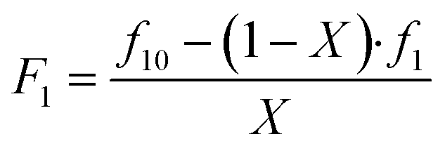(1))

A Gaussian error propagation scheme is used for F, and as the errors in f₁ and f₁₀ are non-negligible, they are also taken into account for the calculation of the error in F₁.³³ We used the excel worksheet provided by the IUPAC working group to calculate errors in F₁ (Fig. S4) for reactivity ratio calculations using Contour, where a measure of uncertainly in form of a JCI is constructed for the obtained reactivity ratios. A sample set of reactions with its starting conditions is given in Table 1, while a representation of their randomised dispensing locations along with conversion heat map and f₁₀ values is shown in Fig. 2b. The data from this table was used in the excel worksheet provided by IUPAC to prepare f₁₀ − X − F − ΔF data for Contour.^18,28 Initially, we used the given f₁₀ values with absolute error estimates of ΔX = 0.005 and Δf₁ = 0.005 for all datapoints (also taking into account the errors of f₁₀) to evaluate the accuracy of the fit provided by Contour for r₁ and r₂. The calculations using Contour resulted in an inadequate fit of the model (95% probability), with the following estimates for the reactivity ratios (M₁ = BMA, M₂ = BA) and the point estimate along with a 95% JCI (Fig. S5):

r₁ = 2.219 (−215 + 0.297), r₂ = 0.367 (−0.058 + 0.074)

Table 1 List of experiments designed for the copolymerisation of BMA (M₁) and BA (M₂) at different BMA initial molar ratios (f₁₀) and AIBN wt%. All experiments are performed at 75 °C for 2 h

Variant	AIBN^a wt%	f10, given^b	f10, experimental^c	f1^d	X^e ^f	F1^g
a AIBN wt% with respect to total monomer mass.b Initial molar ratio of BMA as given in the reaction recipe.c Initial molar ratio of BMA calculated from t0 NMR samples.d Molar ratio of BMA at t1 calculated from NMR.e Overall monomer conversion calculated from NMR.f In cases where NMR malfunction produced a negative conversion result, the experiment was omitted from the dataset used in Contour.g Calculated using eqn (S1) and f10, given values.
1	0.05	0.10	0.09	0.10	0.10	0.13
2	0.05	0.30	0.29	0.26	0.10	0.65
3	0.05	0.50	0.48	0.46	0.16	0.70
4	0.05	0.80	0.78	0.77	0.24	0.90
5	0.25	0.10	0.10	0.01	0.69	0.14
6	0.25	0.30	0.27	0.15	0.59	0.41
7	0.25	0.50	0.49	0.36	0.47	0.66
8	0.25	0.80	0.78	0.72	0.28	1.00
9	0.50	0.10	0.09	0.00	0.91	0.11
10	0.50	0.30	0.29	0.05	0.79	0.36
11	0.50	0.50	0.50	0.29	0.60	0.64
12	0.50	0.80	0.78	0.69	0.60	0.87
13	1.00	0.10	0.10	0.00	0.94	0.11
14	1.00	0.30	0.30	0.00	0.93	0.32
15	1.00	0.50	0.49	0.16	0.83	0.57
16	1.00	0.80	0.80	0.62	0.79	0.85
17	2.00	0.10	0.10	0.00	0.96	0.10
18	2.00	0.30	0.30	0.00	0.96	0.31
19	2.00	0.50	0.49	0.06	0.94	0.53
20	2.00	0.80	0.80	0.42	0.91	0.84

---

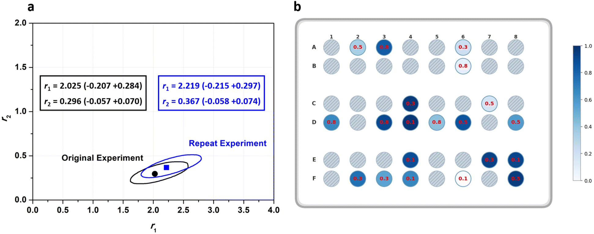Fig. 2 (a) Comparison of JCIs and reactivity ratio estimates for two sets of BMA-BA experiments repeated on different days; (b) representation of random locations chosen by the robot to dispense 20 reaction mixtures across a reactor, with a heat map showing final monomer conversion. Red values represent initial BMA molar ratio (f₁₀).

To address the inadequacy of the fitted model, we then increased the absolute error of measurement for both X and f₁ to 0.05 and repeated the calculations. The result was an adequate fit of the model. Unsurprisingly, this change did not affect the predicted reactivity ratio values or the 95% JCI plot (Fig. S5), since the error between different samples is larger than the individual absolute error values.

Using the automated platform for HTP screening of copolymerisation reactions offers advantages in streamlining the generation of large datasets with minimal manual handling. It is however necessary to ensure repeatability and reproducibility of data produced using the liquid handling robot and across different wells within the reactor. To verify reproducibility, the experiments in Table 1 were repeated on different days. We applied a two one-sided test (TOST) to compare the repeats and used Contour to extract JCIs (Table S2, 21–40). At a delta level of 0.05, TOST indicated that both total monomer conversion and f₁ values were statistically equivalent between repeats (p < 0.01). Moreover, residual analysis of the differences in conversion and f₁ across repeats showed scatter evenly distributed around zero, with no systematic trend. Furthermore, Fig. 2a shows an overlay of the 95% JCIs for the two cases, exhibiting close agreement and strong JCI overlap between the estimated reactivity ratios for the repeated experiment. Overall, this indicates consistent repeat conversion results with no bias across re-randomised wells.

To investigate the effect of using experimental f₁₀ values as opposed to given values – which will directly affect the calculated F₁ values – we used the experimental values given in Table 1 (obtained from t₀ NMR samples) and repeated the analysis. The point estimate along with the 95% JCI for both cases (experimental vs. given f₁₀ values) is presented in Fig. S6. Since no significant difference is observed between the two cases, it was decided to continue all further analysis using given f₁₀ values, while keeping the absolute error for X and f₁ at 0.05 for consistency.

Conducting experiments for 2 h gave us a dataset with low, medium, and high conversion values when a systematically varied AIBN concentration set was used. However, in order to rule out influences of AIBN concentrations on the resulting reactivity ratios, we further evaluated the effect of reaction time on the reactivity ratio predictions. If the AIBN concentration had an effect, one would expect that samples generated for the same monomer conversion at the two different time intervals would not match. To this end, we repeated the same set of experiments as set out in Table 1, only this time we stopped the reaction after 30 minutes rather than 2 h (Table S2, 41–60). Feeding the analysis data from this set to Contour gave us very close reactivity ratio estimations to the original dataset (2 h reaction time) (Fig. S7), underpinning that the chosen reaction times lead to a consistent outcome and are not affected by progressive monomer composition changes. Fig. 3a shows the X − F₁ evolution for different BMA initial molar ratios (f₁₀), combining data from experiment sets with 30 min and 2 h reaction time, also qualitatively showing a very good match between the 30 min and 2 h reaction time data. This proves that our approach of varying AIBN concentrations is valid. Datapoints for different reaction times clearly follow the same trend for different BMA starting molar ratios, while we see an expected convergence of f₁₀ and F₁ values at high monomer conversions. It is noteworthy to point out that these two sets of experiments were conducted several days apart, which further exemplifies the repeatability and robustness of the robotic platform. Overall, this variation proves that the used approach to create samples with different conversions at a set reaction time is valid, and that the reaction time itself has no influence on the result of the procedure.

Fig. 3 (a) Combined F₁–X data for 30 min and 2 h reaction time datapoints for BMA-BA; (b) combined F₁–X data for 79 datapoints obtained for BMA-BA from different experiment sets as shown in Table S2. Lines shown are added to guide the eye, and do not represent a fit of the data.

We mentioned earlier that a total of 20 experiments were set up to ensure minimal evaporation and a reasonable number of NMR samples for evaluation. We were however interested in evaluating the effect of increasing the number of datapoints and the range of f₁₀ on the predicted reactivity ratios for the BMA-BA system. To test this, we conducted a set of experiments using the HTP platform including a more comprehensive f₁₀ range (0.1 to 0.9 with 0.1 increments) with a total of 45 experiments (Table S2, 1–20 & 61–85; Fig. S8). Reactivity ratio values determined using this larger dataset aligned well with the values obtained from the original 20-datapoint dataset. We then compiled several sets as summarised in Table S2 in one dataset, where plotting the F₁–X graph shows a clear trend of f₁₀ approaching F₁ at high conversions for all initial monomer feed ratios (Fig. 3b). We then repeated the analysis with Contour using this dataset. Fig. 4a shows a comparison between the 95% JCI plots for the largest, combined set of 56 datapoints and smaller datasets. Clearly, increasing the dataset size from 20 to 40 datapoints influences the size of the JCI, decreasing it significantly. However, further increasing the dataset size from 40 to 56 does not affect the JCI to a great extent. There is close agreement between the point estimates for BMA-BA reactivity ratios (Fig. 4a) and we therefore opted for the 20-datapoint dataset as a standard evaluation system for further monomer reactivity ratio evaluations.

Fig. 4 (a) Overlay of 95% JCI for different dataset sizes of BMA-BA; (b and c) comparison of reactivity ratios for BMA-BA when indexing of monomers is swapped.

As outlined in the IUPAC guidelines for the evaluation of reactivity ratios, the outcome of a correct statistical technique of evaluation should not depend on the indexing of monomers. Using absolute error values in the calculations of the IUPAC-recommended method – which we have also adopted in this work – ensures that the final reactivity ratios do not depend on the indexing of the monomers. To evaluate this, we used the initial 20-point dataset for BMA-BA in Table 1, and assigned BA as M₁ (Table S3) and repeated the Contour analysis. Fig. 4b and c show a comparison of the 95% JCI and point estimates for reactivity ratios for BMA and BA when indexing is swapped. Satisfyingly, no significant difference is observed between the two cases.

Expanding the scope for the prediction of reactivity ratios

Having established a robust and reproducible automated HTP platform for the investigation of reactivity ratios of binary systems in thermal free-radical copolymerisation using the BMA-BA pair as a case study, we then expanded the monomer pair selection to investigate five other monomer pairs including BMA-St (Table S4), St-BA (Table S5), St-MMA (Table S6), GMA-BA (Table S7), and GMA-St (Table S8). Fig. 5 shows an overview of point estimates for reactivity ratios for these monomer pairs along with their 95% JCIs, covering a diverse range of the reactivity ratio space. In all cases, tight JCIs were obtained, reflecting the strong precision of the nonlinear fitting approach adopted as well as the robotic nature of our method.

Fig. 5 Point estimate and 95% JCIs for reactivity ratios of six different monomer pairs studied using the HTP automated OT-2 platform in this work: (a) BMA, BA; (b) BMA, St; (c) St, BA; (d) St, MMA; (e) GMA, BA; (f) GMA, St.

In addition to the sealed reactor format, reactivity ratios were also determined using a 96-well plate (Greiner, polypropylene), enabling a direct comparison of the two experimental configurations under otherwise equivalent conditions. It was observed that some monomer was lost either due to evaporation during the experiment, or by absorption in the sealant glue. This effect was not observed in the 48 vial setup. While best efforts were undertaken to minimise this monomer evaporation effect, it nonetheless increased the uncertainty of the residual fits, and had an impact on the resulting copolymerisation ratios. This is reflected in generally larger JCIs. In the 96 well plate, roughly twice as many samples are required to generate a result with a similar error level. Despite this, plotting out the copolymerisation curves (Fig. S10–S14) using each set of reactivity ratios reveal that, even if the curves do not match perfectly, the predicted composition trajectories are broadly consistent across both platforms for most monomer pairs investigated. While the individual curves do not show complete overlap, and some results are different from each other with the two methodologies, the match is still relatively good when comparing data with literature, where data spreads of the same order of magnitude are common. The well plate format offers – at least in principle – compelling practical advantages, including increased throughput, accessibility, and reduced cost, rendering it an attractive option as an HTP reactor. Yet, the 48 vial reactor, for which no monomer evaporation was observed at all, is deemed the much more precise option, demonstrated by the absence of monomer evaporation during the experiment (monitored by NMR in absence of AIBN), and by the increased accuracy of the r₁ and r₂ determination using this HTE setup.

By comparing our values measured using the HTP reactor (Table 2) to literature (Table S9), we received a coherent kinetic picture for the chosen monomer pairs, underpinning the efficiency of using harmonised automated experimental conditions and modelling. The reactivity ratios determined in this work show broad agreement with the general trends reported in the literature. However, statistically significant differences were identified for many cited values when assessed against the JCIs reported here. A full comparison is available in the repository provided in the SI, with. As outlined in the condensed Table S11, of the 18 literature entries surveyed across the six monomer pairs, four entries – including two relating to GMA/St and one relating to BMA/St – fell within the 95% JCI of the present measurements for both r₁ and r₂ values. The remaining entries exhibited at least one reactivity ratio from literature lying outside the estimated JCI bounds measured herein. The St/BA and St/MMA systems showed the greatest collective discrepancy, with many literature r₁ values clustering well below the value determined here, though St/BA showed overlap for r₁ and r₂ point estimates in several cases. The BMA/BA, and GMA/St systems showed comparatively closer agreement, with all r₁ and r₂ JCIs overlapping with literature point estimates. These observations motivate consideration of the methodological and experimental factors that systematically distinguish the present work from the cited literature.

Table 2 Summary of reactivity ratios determined for different monomer pairs using the automated platform presented in this work. All experiments were performed at 75 °C for 2 h using toluene as solvent

Monomer pair	r1	r2
M1 = BMA, M2 = BA	2.22	0.37
M1 = BMA, M2 = St	0.58	0.73
M1 = St, M2 = BA	1.23	0.32
M1 = St, M2 = MMA	0.46	0.58
M1 = GMA, M2 = BA	1.76	0.24
M1 = GMA, M2 = St	0.69	0.32

---

The discrepancy between literature and measured values in this work is to some extend expected, and likely attributable to several factors. Firstly, and as previously discussed, most referenced studies employ linearisation methods to estimate r₁ and r₂, which distort the error structure of the Mayo–Lewis equation and are known to yield biased point estimates. It is well-documented within the IUPAC guidelines that such methods deviate significantly from actual values and thus impact accuracy significantly.¹⁸ In contrast, NLLS fitting provides an estimate which is not biased by linearisation and is therefore more representative of reality. In addition, the cited literature reports point estimates without JCIs, which precludes an accurate statistical comparison; nominally different point estimates may therefore in fact be statistically indistinguishable when taking this uncertainty into account. Moreover, differences in reaction medium and operant temperature are likely to contribute to the observed discrepancies. Reactions were conducted here in toluene, with 4 M total monomer concentration at 75 °C, whereas many works use bulk conditions or alternative solvents across broad temperature ranges (25 °C to 170 °C). Preferential solvation of a given monomer is known to shift apparent reactivity ratios relative to bulk values in a system- and solvent-dependent manner, and in addition reactivity ratios are intrinsically temperature dependent due to their relationship to temperature-dependent rate constants.²⁰ This is consistent with the substantial inter-laboratory variation visible even among literature values in polymer chemistry; all experimental works involve errors, and thus it is crucial to establish workflows for HTP and accurate experimentation, while adopting the recommended IUPAC guidelines for modelling of copolymerisation reactions to achieve high-quality datasets for understanding the behaviour of these systems. Ultimately, these discrepancies underscore the urgent need for standardised kinetic benchmarks derived from harmonised HTP protocols. While such datasets are currently unavailable, the platform and methodology presented here offer a clear pathway to acquiring this foundational data and providing the requisite precision for bridging this gap towards future automated polymer discovery.

Conclusions

In the introduction we identified a lack of coherent data for polymerisation systems, especially experimental data for modelling of copolymerisation systems for the determination of reactivity ratios. The proposed automated HTP platform in this work has shown to remove that bottleneck for experimentation, streamlining the generation of experimental data for copolymerisation systems while removing bias and improving repeatability by taking over the tasks commonly performed by the human operator. While data on the reactivity ratios for binary systems exist in literature, inconsistency in method selection, reporting, and often incorrect and inaccurate model selection, results in poor quality data.^18,20f At the same time, under-reporting of experimental errors leads to literature reports that seemingly have a high accuracy, when in reality they are associated with considerable uncertainty. Coherent data generation platforms and consistent evaluation of experimental data according to the latest guidelines for the determination of reactivity ratio helps resolve this persisting issue. As outlined by the recent IUPAC guidelines on methodologies for determining reactivity ratios, there is a direct connection between the ease of experimental methodologies to obtain reactivity ratios and the likelihood of the method seeing increased uptake by polymer chemists. We believe that utilising the HTP automated platform presented here along with the methodology recommended by IUPAC for the analysis of experimental data is a promising pathway for the harmonisation of datasets for a better understanding of the behaviour of copolymerisation systems, as experimental errors are not only minimised, but also accurately assessed. Here we studied the kinetics of different binary monomer systems in an automated fashion, minimising experimental error and bias in the generation of data, while proposing a novel strategy to streamline HTP NMR sample preparation. The ease of generating datasets allowed us to evaluate factors affecting reactivity ratio determination such as dataset size, experimental errors, and repeatability. It was observed that a well-designed experiment set of 20 variants spanning different f₁₀ values using different AIBN initiator concentrations gives a dataset containing f₁₀ − X − F data sufficient to evaluate reactivity ratios for a monomer pair. This approach will in the near future set the scene for the implementation of ML algorithms for a deeper understanding of the complex interplay between factors affecting reactivity ratios in a free-radical polymerisation. This step is crucial to provide the future data basis for advanced ML approaches that correlate monomer structure with reactivity, and the present work must thus not only be seen in the context of robotic HTP experimentation, but as an algorithmic tool towards the application of ML to complex kinetic property predictions.

On a more general note, this study also underpins the power of using robotic sample processing with liquid handlers for detailed kinetic studies. To date, most examples found in this area were restricted to oxygen-tolerant photopolymerisation. The polymerisation-through method we present here using AIBN opens the entire realm of radical polymerisation investigations for the future, and extends the scope of liquid handlers for such studies significantly.

Author contributions

L. Alexander: data curation, investigation, formal analysis, methodology, software, validation, visualisation, writing – secondary draft, writing – review & editing. V. F. Jafari: data curation, investigation, formal analysis, methodology, software, validation, visualisation, writing – original draft, writing – review & editing. T. Junkers: conceptualisation, formal analysis, funding acquisition, methodology, project administration, resources, supervision, validation, writing – review & editing.

Conflicts of interest

There are no conflicts to declare.

Data availability

Data for this article, including Python code and experimental data are available at GitHub: (https://github.com/PRDMonash/A-Robotic-Approach-to-Polymerization-Kinetics-A-Case-Study-on-Copolymerization-Parameter-Estimation.git) and Bridges: (https://doi.org/10.26180/32015067).

Supplementary information (SI): experimental procedures, all primary data and background information on robot programming. See DOI: https://doi.org/10.1039/d6sc02232d.

Acknowledgements

The authors are grateful for funding of the project via the Australian Research Council grant DP240100120.

References

1. (a) J. J. Haven, C. Guerrero-Sanchez, D. J. Keddie, G. Moad, S. H. Thang and U. S. Schubert, Polym. Chem., 2014, 5, 5236–5246; (b) C. Guerrero-Sanchez, L. O'Brien, C. Brackley, D. J. Keddie, S. Saubern and J. Chiefari, Polym. Chem., 2013, 4, 1857–1862; (c) J. J. Haven, C. Guerrero-Sanchez, D. J. Keddie and G. Moad, Macromol. Rapid Commun., 2014, 35, 492–497; (d) C. Guerrero-Sanchez, R. M. Paulus, M. W. M. Fijten, M. J. de la Mar, R. Hoogenboom and U. S. Schubert, Appl. Surf. Sci., 2006, 252, 2555–2561; (e) D. Fournier, R. Hoogenboom, H. M. L. Thijs, R. M. Paulus and U. S. Schubert, Macromolecules, 2007, 40, 915–920; (f) G. K. K. Clothier, T. R. Guimarães, S. W. Thompson, S. C. Howard, B. W. Muir, G. Moad and P. B. Zetterlund, Angew. Chem., Int. Ed., 2024, 63, e202320154; (g) C. Guerrero-Sanchez, S. Harrisson and D. J. Keddie, Macromol. Symp., 2013, 325–326, 38–46; (h) M. Behl, M. Balk, K. Lützow and A. Lendlein, Eur. Polym. J., 2021, 143, 110207; (i) S. Baudis, A. Lendlein and M. Behl, Macromol. Symp., 2014, 345, 105–111.
2. (a) M. Tamasi, S. Kosuri, J. DiStefano, R. Chapman and A. J. Gormley, Adv. Intell. Syst., 2020, 2, 1900126; (b) J. Lee, P. Mulay, M. J. Tamasi, J. Yeow, M. M. Stevens and A. J. Gormley, Digital Discovery, 2023, 2, 219–233; (c) M. J. Tamasi, R. A. Patel, C. H. Borca, S. Kosuri, H. Mugnier, R. Upadhya, N. S. Murthy, M. A. Webb and A. J. Gormley, Adv. Mater., 2022, 34, 2201809.
3. H. Foster, M. H. Stenzel and R. Chapman, Macromolecules, 2022, 55, 5938–5945.
4. V. F. Jafari, Z. Mossayebi, S. Allison-Logan, S. Shabani and G. G. Qiao, Chemistry, 2023, 29, e202301767.
5. V. F. Jafari, S. Nour, R. A. L. Wylie, D. E. Heath and G. G. Qiao, Biomacromolecules, 2025, 26, 311–322.
6. F. Ehlers, J. Barth, P. Vana, P. Vana, R. Storey, Y. Yagci, P. Nesvadba, B. Wayland, G. Moad, A. Goto and R. S. O. Chemistry in Kinetics and Thermodynamics of Radical Polymerization, ed.N. V. Tsarevsky and B. S. Sumerlin,The Royal Society of Chemistry, 2013.
7. J. Chiefari, Y. K. Chong, F. Ercole, J. Krstina, J. Jeffery, T. P. T. Le, R. T. A. Mayadunne, G. F. Meijs, C. L. Moad, G. Moad, E. Rizzardo and S. H. Thang, Macromolecules, 1998, 31, 5559–5562.
8. J.-S. Wang and K. Matyjaszewski, J. Am. Chem. Soc., 1995, 117, 5614–5615.
9. Z. An, ACS Macro Lett., 2020, 9, 350–357.
10. F. R. Mayo and C. Walling, Chem. Rev., 1950, 46, 191–287.
11. (a) E. L. Madruga, Prog. Polym. Sci., 2002, 27, 1879–1924; (b) R. A. Clark and M. P. Shaver, Chem. Rev., 2024, 124, 2617–2650.
12. (a) J.-F. Lutz, M. Ouchi, D. R. Liu and M. Sawamoto, Science, 2013, 341, 1238149; (b) H. J. Harwood, Rubber Chem. Technol., 1967, 40, 427–444.
13. J. P. A. Heuts and B. Klumperman, Eur. Polym. J., 2024, 215, 113215.
14. (a) J. P. A. Heuts, R. G. Gilbert and I. A. Maxwell, Macromolecules, 1997, 30, 726–736; (b) B. S. Beckingham, G. E. Sanoja and N. A. Lynd, Macromolecules, 2015, 48, 6922–6930; (c) G. E. Roberts, M. L. Coote, J. P. A. Heuts, L. M. Morris and T. P. Davis, Macromolecules, 1999, 32, 1332–1340.
15. S. Penczek and G. Moad, Pure Appl. Chem., 2008, 80, 2163–2193.
16. F. R. Mayo and F. M. Lewis, J. Am. Chem. Soc., 1944, 66, 1594–1601.
17. T. Fukuda, Y.-D. Ma and H. Inagaki, Makromol. Chem., 1985, 12, 125–132.
18. A. A. Autzen, S. Beuermann, M. Drache, C. M. Fellows, S. Harrisson, A. M. van Herk, R. A. Hutchinson, A. Kajiwara, D. J. Keddie and B. Klumperman, Polym. Chem., 2024, 15, 1851–1861.
19. (a) E. Van de Reydt, N. Marom, J. Saunderson, M. Boley and T. Junkers, Polym. Chem., 2023, 14, 1622–1629; (b) Y. Wang, Y. Fang, H. Zhou and H. Gao, Molecules, 2024, 29, 4694.
20. (a) N. Kazemi, T. A. Duever and A. Penlidis, Macromol. React. Eng., 2011, 5, 385–403; (b) N. A. Lynd, R. C. Ferrier, Jr. and B. S. Beckingham, Macromolecules, 2019, 52, 2277–2285; (c) S. K. Fierens, P. H. M. Van Steenberge, M. F. Reyniers, D. R. D'Hooge and G. B. Marin, React. Chem. Eng., 2018, 3, 128–145; (d) N. E. Jackson and B. M. Savoie, Macromolecules, 2025, 58, 1737–1754; (e) D. J. Lundberg, L. J. Kilgallon, J. C. Cooper, F. Starvaggi, Y. Xia and J. A. Johnson, Macromolecules, 2024, 57, 6727–6740; (f) K.-I. Takahashi, H. Mamitsuka, M. Tosaka, N. Zhu and S. Yamago, Polym. Chem., 2024, 15, 965–971.
21. M. H. Reis, C. L. G. Davidson and F. A. Leibfarth, Polym. Chem., 2018, 9, 1728–1734.
22. J. Yeow, R. Chapman, A. J. Gormley and C. Boyer, Chem. Soc. Rev., 2018, 47, 4357–4387.
23. (a) X. Hu, G. Szczepaniak, A. Lewandowska-Andralojc, J. Jeong, B. Li, H. Murata, R. Yin, A. M. Jazani, S. R. Das and K. Matyjaszewski, J. Am. Chem. Soc., 2023, 145, 24315–24327; (b) J. Yeow, R. Chapman, J. Xu and C. Boyer, Polym. Chem., 2017, 8, 5012–5022; (c) A. J. Gormley, J. Yeow, G. Ng, Ó. Conway, C. Boyer and R. Chapman, Angew. Chem., Int. Ed., 2018, 57, 1557–1562; (d) X. Wu, L. Xia, Z. Luo, K. Wu, J. Lai, Y. Chen and Y. Xiong, Eur. Polym. J., 2025, 222, 113628; (e) C. Stubbs, T. Congdon, J. Davis, D. Lester, S.-J. Richards and M. I. Gibson, Macromolecules, 2019, 52, 7603–7612.
24. (a) S. Cosson, M. Danial, J. R. Saint-Amans and J. J. Cooper-White, Macromol. Rapid Commun., 2017, 38, 1600780; (b) G. Gody, R. Barbey, M. Danial and S. Perrier, Polym. Chem., 2015, 6, 1502–1511; (c) N. G. Taylor, M. H. Reis, T. P. Varner, J. L. Rapp, A. Sarabia and F. A. Leibfarth, Polym. Chem., 2022, 13, 4798–4808.
25. P. Gurnani, T. Floyd, J. Tanaka, C. Stubbs, D. Lester, C. Sanchez-Cano and S. Perrier, Polym. Chem., 2020, 11, 1230–1236.
26. C. Hagiopol, Copolymerization: toward a systematic approach, Springer Science & Business Media, 1999.
27. G. Ng, S. W. Prescott, A. Postma, G. Moad, C. J. Hawker and C. Boyer, Macromol. Chem. Phys., 2023, 224, 2300132.
28. A. M. van Herk, in Software package Contour issue 2.4.0, accessed 03/04/2024 Contour 2.4.0.
29. M. Fineman and S. D. Ross, J. Polym. Sci., 1950, 5, 259–262.
30. T. Kelen and F. Tüdős, React. Kinet. Catal. Lett., 1974, 1, 487–492.
31. (a) R. A. Hutchinson, B. Klumperman, G. T. Russell and A. M. Van Herk, Can. J. Chem. Eng., 2022, 100, 680–688; (b) M. Dube, R. A. Sanayei, A. Penlidis, K. F. O'Driscoll and P. M. Reilly, J. Polym. Sci., Part A: Polym. Chem., 1991, 29, 703–708.
32. A. M. van Herk, J. Chem. Educ., 1995, 72, 138.
33. (a) A. M. Van Herk and T. Dröge, Macromol. Theory Simul., 1997, 6, 1263–1276; (b) M. Buback, T. Dröge, A. V. Herk and F.-O. Mähling, Macromol. Chem. Phys., 1996, 197, 4119–4134.

---

Footnote

† These authors contributed equally to this work.

---