A fresh perspective on the role of band bending, and related contributors, in light-driven production of electricity and chemicals

Abstract

It is widely known that semiconductor-based solar energy conversion could power our planet. This is in part because high-quality semiconductor structures are unrivalled in their ability to separate photogenerated electrons and holes. One effective approach to achieving this photoinduced charge separation relies on a phenomenon known as “band bending”. But details to justify why band bending results in photoinduced charge separation are more complex than often appreciated. This underappreciation is an impediment to the rational, hypothesis-driven design of next-generation approaches to solar energy conversion. Herein we show, by means of derivations rooted in physical chemistry, that several phenomena – not just band bending – can facilitate photoinduced charge separation, and that each is influenced by nonequilibrium species concentration and a parameter, such as diffusion coefficient or rate coefficient, that introduces dynamics. To help visualize the impact of each phenomenon, we introduce plots that depict their contributions as free energy, force, flux, force constant, and rate. We reveal that spatial dopant distributions that define band bending are predictors of initial photogenerated species transport rates. But charge separation alone does not guarantee high-efficiency operation. A photogenerated change in energy that is freely available to do useful work is also essential, and is strongly dependent on semiconductor optical properties and reaction kinetics. Notably, this information reveals that specificity of interfacial chemical reactions – even when they are not preceded by charge separation elsewhere – can result in efficient solar energy conversion. We expect that this tutorial will guide researchers in their pursuit to uncover new mechanisms for light to perform useful work.

---

Broader context

Without a strong foundation in core concepts, researchers are left to guessing and a reliance on serendipity to invent new ways of performing desired tasks. We can, and must, do better when it comes to developing next-generation sustainable energy systems. Hypothesis-driven research and development is a stronger strategy to make advancements in the use of renewable energy sources to power our planet in ways that are economically and environmentally friendly. It relies on intentional innovation followed by implementation of the scientific method. This strategy, however, requires a deep understanding of the facts and a shared technical language across a multidisciplinary space. To help facilitate this, we developed a tutorial on photoinduced charge separation. In it, we present field-agnostic thermodynamic and kinetic concepts rooted in the chemical sciences and engineering. We demonstrate that there are many ways to achieve photoinduced charge separation, a general prerequisite to performing useful work with light. Only with fundamental knowledge can researchers rapidly invent, and vet the importance of, new approaches that are so urgently needed.

The Sun provides to Earth enormous amounts of clean radiant energy,¹ far exceeding humanity's energy needs.^2–4 This fact has motivated scientists and engineers to develop engines that efficiently convert sunlight into other forms of energy, by what have been termed sunlight-to-X processes.⁵ Innovative approaches are an outcome of the wide range of viewpoints considered, which span the physical and biological sciences to engineering, and provide hope that someday soon we might discover an approach that is a gamechanger for sustainability.

The most efficient engines for sunlight-to-X energy conversion use semiconductor photoabsorbers. Absorption of light by these photoabsorbers results in a 1 : 1 stoichiometric increase in the concentration of negatively-charged mobile electrons (e⁻), in electronic states that form the conduction band (cb), and positively-charged mobile holes (h⁺), due to removal of electrons from electronic states that form the valence band (vb). It is generally desired that these photogenerated mobile charged species separate and are then collected for sunlight-to-X energy conversion (X = electricity, chemicals) — alternatively, they can recombine (X = heat, light), which is not generally desired.

A major advance in sunlight-to-electricity energy conversion came in the mid-twentieth century with the advent of the semiconductor pn-junction (Fig. 1a).⁶ Diffusion of specific charge-neutral dopant atoms into a crystalline, elemental semiconductor lattice, e.g. Si, resulted in spontaneous formation of a p-type region, enriched in positively-charged mobile h⁺ and immobile charge-compensating negatively-charged ionized dopants (−), and an adjacent n-type region, enriched in negatively-charged mobile e⁻ and immobile charge-compensating positively-charged ionized dopants (+). These thermalization processes in the dark generated the p-type and n-type regions, but it is the related electrochemical equilibration process that highlights the ingenuity of the formed pn-junction. Transport of dopant-derived mobile e⁻ and h⁺, followed by their spontaneous 1 : 1 stoichiometric recombination, resulted in a spatial charge imbalance due to the remaining immobile ionized dopants, and therefore electric fields and electric potential differences within the semiconductor (Fig. 1a and b) — it is these electrostatic properties that aid in photoinduced charge separation.

Fig. 1 Electrostatic diagrams and band diagram. Depictions of properties of an equilibrated semiconductor pn-homojunction, which is approximated, as is typical, to have a sharp interface, as a so-called abrupt junction,¹² between regions that each have a spatially invariant concentration of immobile dopants. In this case, the immobile dopants are assumed to be fully ionized and at the same concentration on both sides of the junction. The pn-junction is known as a homojunction, because the semiconductor is homogenous across the interface. The pn-junction design is one where a spatially invariant rate of photon absorption to generate nonequilibrium concentrations of mobile charged species (not shown) would result in transport of mobile electrons (e⁻) to the right and mobile holes (h⁺) to the left. (a) C̲o̲m̲p̲l̲e̲t̲e̲ e̲l̲e̲c̲t̲r̲i̲c̲ c̲i̲r̲c̲u̲i̲t̲ that includes a semiconductor pn-homojunction along with an exemplary equilibrated e̲l̲e̲c̲t̲r̲i̲c̲ p̲o̲t̲e̲n̲t̲i̲a̲l̲ d̲i̲a̲g̲r̲a̲m̲. This representation includes the entire distribution of system electric potential, , along the closed path of charge transport through an ionic pathway (e.g. an electrolyte phase) or an additional electronic pathway (shown with the example of metals (M), each chosen to generate no electric fields, i.e., at the interface with each of the p-type and n-type semiconductor). (b) Equilibrated e̲l̲e̲c̲t̲r̲o̲s̲t̲a̲t̲i̲c̲ d̲i̲a̲g̲r̲a̲m̲, highlighting (blue box) that some of the electric potential information is also shown in panels a and c. This representation assumes the so-called depletion approximation¹² for the semiconductor, where immobile ionized dopants constitute charge densities, (each as the product of concentration, charge number, and the Faraday constant), across the pn-homojunction (−/+) that screen each other, without secondary considerations of mobile h⁺/e⁻ at the extremes of these respective regions. This closely associated charge screening — over what is termed the depletion region — confines electric fields, , whose values then vary linearly in space, i.e. are diagonal lines, and with relations to and as the gradient of the parabolic electric potential, i.e., and as the integral of the ratio of the charge density to the static permittivity, i.e., each in one spatial dimension, x. (c) Equilibrated t̲r̲a̲d̲i̲t̲i̲o̲n̲a̲l̲ b̲a̲n̲d̲ d̲i̲a̲g̲r̲a̲m̲ at electrochemical equilibrium, including free energies for each of mobile e⁻ and h⁺ (shown as Fermi levels, i.e. E_F,e⁻ = +[small mu, Greek, macron]_e⁻ and E_F,h⁺ = −[small mu, Greek, macron]_h⁺) and internal energies of the valence-band edge, , and conduction-band edge, , with bands of electronic states as solid colors. Contributions due solely to are depicted, as is typical, by the energy of the local vacuum located just outside the system and with zero kinetic energy, , in reference to a vacuum state approaching an infinite distance away from the system, with zero kinetic energy, and with spatially invariant energy, .

Over time it became popular to illustrate electric potential differences in semiconductors as “band bending” on a plot of energy as a function of location in one spatial dimension, as an energy (“band”) diagram. Today, “band diagrams” are widespread in articles describing sunlight-to-X energy conversion, underscoring the impact that electric-field-driven charge separation has had on understanding efficient solar cell design. However, this band-bending description is often too simple and only sometimes predictive of whether mobile charged species will undergo photoinduced charge separation. While the cause–effect relationship between the presence of electric fields and separation of mobile species bearing opposite charge is logical, it obfuscates a more general understanding of (sun)light-to-X energy conversion processes. This issue is compounded by the presentation of the band diagram itself, which was designed using the language of solid-state physics for applications when X = electricity. By overlooking principles central to chemistry that are particularly important when X = chemicals, this historical terminology impedes opportunities to rationally innovate — the language associated with band diagrams is not traditionally used by all scientists and engineers. Our hope is that this tutorial promotes not only a deeper appreciation of opportunities available to researchers studying light-to-X energy conversion, but also invigorates them to embark on multidisciplinary collaborative efforts that may lead to urgently needed breakthroughs.

Key lessons to be learned

To rationally innovate in light-to-X energy conversion, it is important to understand the principles that define how absorption of light increases the energy of the system, some of which is freely available to do useful work at a rate determined by species flux — in terms of electrical work, i.e. X = electricity, this is how voltage is related to current, as has been reported many times previously.^1,7–12 Using photogenerated free energy to explain downstream actions is the foundational physics way to teach light-to-electricity energy conversion. However, as an alternative pedagogy based on general thermodynamics and kinetics, herein we take a different approach. Section I defines free energy contributions to light-to-X energy conversion processes. Section II introduces how a system evolves in time based on several physical interpretations of transport. Section III explains causes of photogenerated species flux. Section IV introduces photogenerated free energy and useful work. Section V unifies this information using volumetric rates. And ultimately, Section VI details approaches that we think will help facilitate rational innovations in light-to-X energy conversion. In doing so, we highlight the following important facts:

(1) Although band diagrams illustrate differences in electric potential, they only indirectly show other contributors to free energy, such as species concentrations. Spatial variation in species concentration results in net diffusion, which in the dark opposes transport resulting from band bending that was described above, and allows these diagrams to represent the condition of electrochemical equilibrium;

(2) Photoinduced transport and charge separation can readily be driven by more than differences in electric potential, including differences in standard free energy, state density, activity coefficient, temperature, and kinetics. These contributors are not depicted directly on band diagrams, and none of them even require bands of electronic states;

(3) Even differences in free energy that suggest mobile species bearing opposite charge transport in the same direction can result in photoinduced charge separation because of species ensemble diffusion coefficients and reaction rate coefficients. While these contributors are not depicted – even indirectly – on band diagrams, they are critical because each introduces dynamics into what is otherwise only a depiction of spontaneity; and

(4) Differences in free energy, i.e. energy that is freely available to do useful work, are foremost required for light-to-X energy conversion, providing the driving force for charge separation that can spontaneously generate photovoltages and photocurrents. These free energy differences may not be directly deducible from internal energies that dominate band diagrams (Fig. 1c) without consideration of properties that are not shown: probabilities to absorb light, reaction kinetics, and photon fluxes from the surroundings.

Before we proceed to share mathematical and physical details that are critical to understanding photoinduced charge separation and light-to-X energy conversion, we present four thought experiments to summarize important overall conclusions from this tutorial.

(i) Imagine you have a semiconductor photoabsorber. At electrochemical and thermal equilibrium, each species ensemble at any location in the semiconductor exhibits, on net, zero transport flux and simultaneously zero reaction rate. Then, upon absorption of sunlight, concentrations of e⁻ and h⁺ ( and ) each increase by an equal amount from its equilibrium value. How much useful work can be performed per e⁻–h⁺pair? As described in detail below, the answer is not the bandgap energy, but rather the change in free energy due to photoexcitation within the photoabsorber. At low light intensity, concentrations of species are altered only somewhat from their equilibrium values, meaning that the free energy generated is relatively less — increased light intensity generates greater free energy difference. This clarifies that internal energies shown on band diagrams are only indirect indicators of light-to-X energy conversion efficiency.

(ii) While absorption of photons to generate nonequilibrium species concentrations is self-evidently important for light-to-X energy conversion, photoinduced charge separation is also critical. Electric fields drive e⁻ and h⁺ to transport in opposite directions and, as described in detail below, their fluxes depend mathematically on the concentration of each, i.e. or , respectively. Transport resulting from a concentration gradient, i.e. diffusion, also depends on positional or , but with no directional dependence based on species charge. How then can absorption of sunlight homogeneously across a photoabsorber result in charge separation? It is because absorption that is spatially homogeneous increases and by an equal amount everywhere, resulting in no net change in species flux due to diffusion. This contrasts with species flux due to electric fields, which, being directional based on both the sign of the electric field and species charge, results in photoinduced charge separation. Moreover, initial photogenerated species fluxes are directly proportional to the underlying distribution of electric fields. This clarifies the critical role that band bending can have in light-to-X energy conversion processes.

(iii) But one can envision a scenario where e⁻ and h⁺ are driven in the same direction, each by a force that also depends on or . In this case, how can absorption of sunlight homogeneously across a photoabsorber result in charge separation? As described in detail below, mass-transfer processes rely on more than the concentration of species, i — they also depend on its diffusion coefficient, . Species diffusion coefficient is the mass-transfer equivalent of the rate coefficient, , for a reaction, r. If the diffusion coefficient differs for e⁻ and h⁺ they will separate – even though they transport in the same direction – because one species ensemble will move faster than the other. This highlights that band bending, and related thermodynamic contributors, are not the only ways to achieve photoinduced charge separation.

(iv) Chemical kinetics and photochemistry can result in photoinduced charge separation, even in the absence of other effects. Assume that the rate of a desired reaction, r, is defined by the mass-action expression , while that for an undesired reaction, r′, is defined as . In this case, when will a selective reaction occur, which by definition results in charge separation? Well, analogous to charge separation resulting from differences in for two species ensembles, absorption of sunlight results in selectivity for over when . And as described in detail below, this outcome is independent of the spontaneity of each reaction at standard state, as long as the reverse back reaction is slower than reaction products are extracted from the reaction volume. This establishes clear design rules for how photochemistry, even in the absence of a semiconductor, can be effective at light-to-X energy conversion.

We now proceed to explain each of these scenarios – hopefully with sufficient rigor – such that you, too, arrive at these same conclusions. Newcomers to the field may find it useful to first familiarize themselves with historical aspects of semiconductor-based solar energy conversion,^1,9–12 which experts in the field likely know well. Independent of prior expertise, we expect that newcomers and experts alike will gain a new appreciation for some concepts in light-to-X energy conversion by reading this tutorial.

I. Electrochemical potential as the free energy parameter

A. Information included in, and omitted from, band diagrams

The process of light-to-X energy conversion begins with absorption of photons to generate a nonequilibrium concentration of excitons, irrespective of whether the photoabsorbing phase is a semiconductor, a more molecular species, or otherwise. When the phase effectively screens charges, meaning it has a large static permittivity (e.g. silicon, metal oxides, water), each exciton rapidly dissociates into a reduced state (e.g. semiconductor conduction-band electron, reduced dye molecule, reduced electron acceptor) and an oxidized state bearing opposite charge (e.g. semiconductor valence-band hole, oxidized dye molecule, oxidized electron donor). Charge separation requires that these nonequilibrium ensembles of mobile charged species must move differentially with respect to each other, constituting current flow. In many semiconductor devices, the invoked explanation for this photoinduced charge separation is band bending, which herein we define as spatial differences in electric potential, , that commonly exist near phase boundaries, e.g. semiconductor interfaces (Fig. 1). But why is it that band bending results in charge separation when illuminated? The answer may appear to be straightforward based on a band diagram (Fig. 1c): electric fields drive oppositely charged mobile species in opposite directions. But there is more to this than meets the eye. This explains how a solar cell can work, but it hides critical details that support why in fact a solar cell does work. To introduce this conundrum, and its resolution, we explain the origin of the band diagram using a thermodynamic framework motivated by Ross and Hsiao⁸ for a common semiconductor, e.g. crystalline silicon, operating as a photovoltaic solar cell.

A solar cell uses the energy in sunlight to perform electrical work, i.e. X = electricity as current flow through an additional electronic pathway that forms a closed circuit. This circuit is a closed system, meaning that matter cannot enter or exit it. In the dark, we can assume that species in this system are at electrochemical equilibrium, and are in thermal equilibrium with the local surroundings through, at a minimum, exchange of photons.¹³ Under these equilibrium conditions, the free energy difference for transport and reactivity are each equal to zero, and therefore, species concentrations do not change, on net, over time. That is, although species are both chemically and spatially dynamic, any time-averaged snapshot will present the same spatial distribution for each species ensemble. But if band bending is present in the dark (Fig. 1), how are all populations of mobile species at equilibrium — in other words, why are mobile charged species not propelled in different directions due to spatial differences in electric potential? The answer is that the electric field, , as the gradient of electric potential, i.e., in one spatial dimension, x, (Fig. 1b, middle plot) is just one of several driving forces for species transport and reactivity. Another driving force results from the gradient of chemical potential, i.e. for each species ensemble, i. Chemical potential, μ_i, is an important state function that, analogous to electric potential for charged species, is necessary to describe the contribution of that species ensemble to the spontaneity of a process.¹⁴ While and μ_i are of similar importance, we find that most light-to-X researchers discuss μ_i less often. Motivated by this, we firmly support proposed pedagogy that introduces μ_i early in classroom education, and at all levels of collegiate study,¹⁴ so that it can be used logically as the foundation for other concepts in thermodynamics, kinetics, and transport.

But given the similar importance of system electric potential, , and species chemical potential, μ_i, where are contributions due to species chemical potential shown on a band diagram? While it may seem surprising, the answer is that μ_i are not depicted directly (Fig. 1c) — instead, they are inferred from band diagrams. Thus, while band diagrams are elegant, their emphasis on over μ_i illustrates tradeoffs made for simplicity, and may have contributed to less frequent usage of μ_i by light-to-X researchers. In light of this, band diagrams do instead illustrate overall net spontaneity. The free energy for each major species ensemble to transport and/or react is shown as an associated electrochemical potential, [small mu, Greek, macron]_i, state function through depiction of “Fermi levels”, i.e. E_F,i (Fig. 1c and 2a). With the collective information presented in band diagrams, i.e. E_F,e⁻ = +[small mu, Greek, macron]_e⁻, E_F,h⁺ = −[small mu, Greek, macron]_h⁺, and , values of μ_i are trivial to deduce with knowledge of the following equation,

where z_i is the species charge number and q is the elementary charge (which equals as the Faraday constant divided by the Avogadro constant), and specific parameters include a subscript x to remind the reader that each has an explicit dependence on location — for brevity, these subscripts are generally omitted in the body of the text.

Fig. 2 Electrochemical potential diagrams. Alternative depictions of properties of an equilibrated semiconductor pn-homojunction described in Fig. 1 and color-coded analogous to Fig. 1c. (a) Equilibrated e̲l̲e̲c̲t̲r̲o̲c̲h̲e̲m̲i̲c̲a̲l̲ p̲o̲t̲e̲n̲t̲i̲a̲l̲ d̲i̲a̲g̲r̲a̲m̲, which is an analog of a band diagram (Fig. 1c) but is based entirely on free energy contributions, including replacing Fermi levels, E_F,i, with their respective electrochemical potentials, i.e. [small mu, Greek, macron]_e⁻ = +E_F,e⁻ and [small mu, Greek, macron]_h⁺ = −E_F,h⁺, and showing species standard concentration chemical potential, . By not depicting (shown in Fig. 1c), and if these curves had not been colored, individual contributions due to and could not be deduced. (b) Equilibrated c̲o̲m̲p̲r̲e̲h̲e̲n̲s̲i̲v̲e̲ e̲l̲e̲c̲t̲r̲o̲c̲h̲e̲m̲i̲c̲a̲l̲ p̲o̲t̲e̲n̲t̲i̲a̲l̲ d̲i̲a̲g̲r̲a̲m̲, including , species chemical potential, μ_i, and species concentration, , and showing that free energy contributions due to μ_i and result in the condition of electrochemical equilibrium as indicated by a spatially invariant [small mu, Greek, macron]_i for each of mobile electrons (e⁻) and holes (h⁺). Each curly brace near the [small mu, Greek, macron]_i horizontal line highlights the curves that represent properties for e⁻ (right) and h⁺ (left).

B. Chemical potential as the central concept in energy conversion

A species ensemble at electrochemical and thermal equilibrium undergoes no net transport. Under this condition, [small mu, Greek, macron]_i is spatially invariant, and therefore constant, such that the shape of μ_i is exactly band bending inverted, i.e. (Fig. 2b). Indirectly, this also informs species concentration, , because, as shown below, μ_i is linearly related to the logarithm of (Fig. 2b). With an understanding that μ_i and are inferred from band diagrams, it is clear why only those familiar with such diagrams could use them to deduce causes of photoinduced charge separation and light-to-X energy conversion. But details are necessary so that any researcher can interpret band diagrams and accurately answer the overarching question: How does absorption of light in a region with band bending drive nonequilibrium concentrations of mobile charged species to separate — in other words, why doesdrive faster net charge transport of e⁻and/or h⁺than from equal and opposite?

Explaining causes of photoinduced charge separation – at a level that provides mechanistic details grounded in chemical and physical intuition – warrants presentation of additional fundamental equations. Before doing so, it is instructive to recall that the spontaneity of all processes, including mass action (chemical reactions) and mass transfer (species transport), are underpinned by the Second Law of Thermodynamics, i.e. processes occur, on net, that statistically increase the entropy of the Universe.¹⁵ Equivalently, processes net occur when they are accompanied by a decrease in the energy of the system that is freely available to perform useful work, from an initial state to a final state — i.e. their difference, Δ, is negative at a constant system temperature and pressure (for Gibbs free energy, ΔG_sys) or temperature and volume (for Helmholtz free energy, ΔA_sys). Spontaneity of a process can also be defined by a decrease in system internal energy or enthalpy, when system entropy remains constant, at a respective constant system volume (for internal energy, ΔE_sys) or pressure (for enthalpy, ΔH_sys).¹⁵ To better understand causes of photoinduced charge separation, consider a hypothetical scenario that includes no chemical reactions and where only transport is operative. The spontaneity of transport for each species ensemble is defined as where the partial derivative captures the change in free energy of the species ensemble, albeit between two positions, and in this regard takes the place of Δ above. While the sign of alone dictates the net direction of species ensemble transport, to conceptualize specific chemical and physical aspects that underlie [small mu, Greek, macron]_i, beyond those shown in eqn (1), we present the most common definition of the chemical potential for a species ensemble, μ_i, in one spatial dimension, x, as follows,^1,15

where species ensemble, i, has a standard chemical potential, , temperature, T_i, activity, a_i, activity coefficient, , and standard concentration, , and k_B is the Boltzmann constant (which equals where R̲ is the gas constant). As written, the unit for μ_i is energy per entity, where exemplary entities include a particle, e.g. i = e⁻, h⁺, photon, or a molecule, as is common in chemistry. Additional details are presented in Box 1.

Box 1. Reaction thermodynamics and its relation to chemical kinetics

Eqn (2) can be derived using fundamental thermodynamics or statistical mechanics.¹⁵ It underlies the analogous equation that defines spontaneity of a chemical reaction, r, many of which occur at a constant system temperature, T_sys, and pressure, p_sys, i.e. where ΔG_r is the molar Gibbs free energy difference upon infinitesimally progressing a reaction to form products at the expense of the reactants.¹⁶ This fact is illustrated by another expression for ΔG_r as the sum of μ_i for each species ensemble that participates in the reaction weighted by its signed stoichiometric number, ν_i,¹⁵ and multiplied by the Avogadro constant, N_A (Fig. 3). Multiplication by N_A highlights that it is common to represent free energy as an intensive property per entity in solid-state physics, while it is common to represent it on a molar basis in chemistry. Also, is the reaction quotient and K_r = Q_r,eq is the equilibrium (eq) constant, meaning when all a_i satisfy an equilibrium condition, i.e. ΔG_r = 0, and which in turn defines the standard value for .¹⁵ Moreover, and are the concentration reaction quotient and the concentration equilibrium constant, respectively — and intrinsically contains contributions due to and . Also, notably, as the ratio of the reaction rate constants in the forward and backward directions,¹⁵ and therefore, is the analogous ratio of reaction rates — reciprocating results in for reactants of the reaction in the numerator and for products of the reaction in the denominator. We prefer the phrase ‘rate coefficient’ over ‘rate constant’ to unify its naming convention with related diffusion coefficient and mass-transfer coefficient. While we appreciate that other so-called ‘constants’, e.g. equilibrium constant and force constant, are also influenced by local electric potential difference, temperature, etc., we do not rename them as ‘coefficients’ herein. Irrespective, the importance of rate coefficients, the usefulness of concentration equilibrium constants to mitigate arbitrary choices of reference values, and considerations for choosing standard concentrations are each described in more detail below.

Fig. 3 Physicochemical properties in light-to-X energy conversion. The electrochemical potential, [small mu, Greek, macron]_i, (upper left) defines the free energy of each species ensemble, i, at any position, x, herein in one spatial dimension. For species transport (solid arrow path), the opposite of the gradient of [small mu, Greek, macron]_i, as its first derivative in space, (right) equals the force exerted by the species ensemble, F_i, that when divided into thermal energy per entity, k_BT_i, (right) results in a signed characteristic length, L_i, over which the work done by that force equals thermal energy. Division into species diffusion coefficient, , (down) results in species mass-transfer coefficient, , that when multiplied by species concentration, , (left) equals species molar flux, N_i. The opposite of the gradient of N_i, as its first derivative in space, (down) equals the volumetric rate of change of the species concentration, R_i, that when divided by (right) equals the species rate coefficient, . For a chemical reaction, r, (dashed arrow path) that involves multiple species ensembles, the sum of [small mu, Greek, macron]_i (upper left) for each species ensemble, i, weighted by its signed stoichiometric number, ν_i – and the Avogadro constant, N_A, for conversion to a molar basis – a specific position, x, (down) equals the molar Gibbs free energy difference, ΔG_r, at a constant system temperature and pressure. The value of ν_i is positive for each reaction product and negative for each reactant, and any contribution from cancels out in the arithmetic because chemical reactions are charge neutral. Division by the opposite of molar thermal energy (i.e. −R̲T_r), and serving as the power of an exponential, (down) equals where 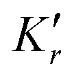is the concentration equilibrium constant and is the concentration reaction quotient, and whose numerator and denominator (right) can each be represented as a unidirectional volumetric reaction rate in the forward (f), R_r,f, or backward (b), R_r,b, direction. Analogous to R_i, division of each R_r by for each species involved in that direction of r, and raised to its respective ν_i, (right) equals the respective unidirectional reaction rate coefficient, . The symbol ■ stands for the expression in the preceding box and the symbol □ stands for i (for species transport) and r, f or r, b (for a chemical reaction in its respective forward or backward direction). The unit for each parameter is reported in Tables 1 and 2.

While μ_i includes effects due to all forces of Nature, i.e. gravity, electromagnetism, the weak force, and the strong force, additional terms are often explicitly added to eqn (2) when their specific effects can be reasonably approximated or measured separately from their influence on μ_i — but effects cannot be double counted. This is the logic behind eqn (1), which captures the influence of on transport at the classical level,^14,17 and is expanded as follows by substituting eqn (2) into it,

where n_i is species ensemble amount – and converts the basis of energy unit for extensive G_sys (i.e. for the entire system) into that for intensive [small mu, Greek, macron]_i (i.e. per entity) – and partial derivative subscripts indicate state functions assumed to be held constant. We indicate as the partial Gibbs free energy per entity, because this condition of constant T_sys and p_sys is common in chemistry. Analogous relations exist for A_sys, E_sys, and H_sys,¹⁵ when other system state functions are held constant — the assumption of constant system volume is in particular reasonable for most semiconductors. Moreover, eqn (3) highlights that µ_i has explicit reference states as and , while the reference state for is implicit. Additional details are presented in Box 2.

Box 2. Electrostatics and reference states

While changes in at the classical level (eqn (3)) are often sufficient to explain observations in light-to-X energy conversion, this approximation is likely inaccurate when the magnitude of is large, meaning electric fields are large, resulting in, for example, Stark effects,¹⁸ enhanced rates of heterolytic water dissociation,^19,20 and/or increased species conductivities.²¹ Thus, while eqn (3) separates some effects due to μ_i and , it does not separate all of them — electrostatic effects of inherently influence μ_i at the quantum mechanical level. This is compounded by the fact that is mathematically dependent on the spatial distribution of all charged species, via the Poisson equation,²² and where the spatial distribution of each species in influenced by its μ_i — the interdependence of and μ_i makes it difficult to intuit mechanistic details of processes in light-to-X energy conversion. An additional point arising from eqn (3) relates to reference states — describes the reference state for μ_i yet there is no formal indication of a reference state for . While a spatially invariant reference state for can be defined,^23,24 for the purposes of light-to-X energy conversion such a definition is unimportant. This is because , as defined in eqn (3), only affects mass-transfer fluxes and, as described in Section II.A below, its influence always depends on a difference in between two positions — this means that a chosen reference value cancels out in the arithmetic. But why then doeseqn (3)include a reference state forμ_ias? This is because, in addition to affecting mass-transfer flux between positions, μ_i also defines reaction free energy differences at each position via stoichiometry-weighted sums of μ_i for several different species ensembles (Box 1). This combination of μ_i means their relative values, including those of their reference states for based on chosen must be consistent with the appropriate, experimentally-verifiable thermodynamics of each reaction. These outcomes are a consequence of being defined at the system level, while is defined for each species ensemble.

The thermodynamic relations indicated by eqn (1)–(3) motivated us to recast the traditional band diagram in terms of solely free energy contributions, i.e. not internal energies, as an analogous electrochemical potential diagram (Fig. 2a) that can then be easily expanded to a comprehensive electrochemical potential diagram (Fig. 2b) — it illustrates several free energy contributions that dictate overall spontaneity, and therefore effectiveness, of photoinduced charge separation. This approach complements the traditional solid-state physics representation with one that is more chemical in nature.

II. Physical interpretations of transport

A. Transport of mobile charged species by associated forces

As described above, the spontaneity of a transport process for a species ensemble, i, in one spatial dimension, x, is captured by the gradient of [small mu, Greek, macron]_i, as . Inspection of the unit for this factor, per entity (i.e. Joules per distance, or equivalently 10⁻² Newtons, when J cm⁻¹), shows that it can be considered a force of opposite sign, F_i. The sign of this force wholly defines the net direction of mass transfer for that species ensemble. But to quantitatively determine the net magnitude of mass transfer for that species ensemble – which is the critical property required to understand charge separation – its diffusion coefficient (; unit: cm² s⁻¹) and (unit: mol cm⁻³ = 10⁻³ M) are needed. This is clear from the following equation, which defines the net molar mass-transfer flux for a species ensemble (N_i; unit: mol cm⁻² s⁻¹) along one spatial dimension, x, through a cross-sectional area (unit: cm²),²⁵where is a signed characteristic length (L_i; unit: cm) over which the difference in [small mu, Greek, macron]_i is equal to thermal energy per entity, i.e. k_BT_i, and is a mass-transfer coefficient (; unit: cm s⁻¹), whose unit is consistent with a velocity. Each symbol was chosen to uniquely identify a parameter and each unit was chosen to aid in dimensional analysis, even though some are less common (Tables 1 and 2) — this is a consequence of simultaneously presenting ideas from multiple disciplines where the same symbol is used for different parameters, e.g. J for current density and mass-transfer flux, for rate coefficient and mass-transfer coefficient, e for the mathematical constant and elementary charge.²⁶ (Subscripts used herein are reported in Table 3.) Irrespective, dimensional analysis for reveals that each length dimension of the cm² portion of its unit is along the same Cartesian coordinate, and therefore, it does not represent an area — is statistically half of the mean squared displacement in one spatial dimension, meaning the variance in position, over time.²⁵ Moreover, the product of and either or are reminiscent of equations for mass action in chemical kinetics, where and are replaced by the rate coefficient (; unit: M^{(1−unidirectional total reaction order)} s⁻¹) for reaction, r. These three parameters, i.e. diffusion coefficient as (cm² s⁻¹), mass-transfer coefficient as (cm s⁻¹), and rate coefficient as (M^{(1−unidirectional total reaction order)} s⁻¹), (Fig. 3, right column) are important when trying to rationally innovate in light-to-X energy conversion, because each alone introduces dynamics as a frequency (i.e. s⁻¹) to net undergo any process — for thermally-activated processes, each of these parameters can also be reasonably described by an Arrhenius expression.²⁷ Moreover, species free energy as [small mu, Greek, macron]_i (J entity⁻¹), force as F_i (J cm⁻¹ entity⁻¹), characteristic length as L_i (cm), flux as N_i (mol cm⁻² s⁻¹), and rate as R_i (mol cm⁻³ s⁻¹) (Fig. 3, clockwise path) are physicochemical properties that are presented throughout this tutorial to help clarify and explain mechanisms of photoinduced charge separation and light-to-X energy conversion. Additional details are presented in Box 3.

Box 3. Conductivity and mobility

The importance of the product is recognized in the context of performing electrical work by its role in defining the species ensemble conductivity (σ_i; unit: Ω⁻¹ cm⁻¹), i.e.,^15,25 where the two z_iq (or z_iF̲) factors convert (i) thermal energy, due to k_BT_i (or R̲T_i), into its electrical equivalent voltage, V_i, and (ii) mass-transfer flux, due to , into its electrical equivalent current, I_i, which when divided by cross-sectional area is equal to current density, J_i = z_iF̲N_i. The equation for σ_i also supports that it is directly related to species ensemble mobility (; unit: cm² s⁻¹ V⁻¹), because for nonmetallic, i.e. nondegenerate, doped semiconductors and low ionic strength electrolyte phases, based on the Einstein(–Smoluchowski) relation.^12,21,25

Table 1 English symbols chosen to represent quantifiable properties, and indicated common units†

English symbol	Unit	Description
†Properties that are dimensionless are marked with ‘—’ in the Unit column.
a	—	Activity
A	J	Helmholtz free energy (for a system)
	mol cm^−3 = 10^−3 M	Molar concentration
	mol cm^−3 = 10^−3 M	Standard molar concentration
d	cm	Distance
	cm^2 s^−1	Diffusion coefficient
	J or J entity^−1	Internal energy (for a system or a band diagram)
	V cm^−1	Electric field
EF	J entity^−1	(Quasi-)Fermi level (for a band diagram)
E°′	V	Formal potential
f	J cm^−2 entity^−1	Force constant
F̲	C mol^−1	Faraday constant
F	J cm^−1 entity^−1 = 10^−2 N entity^−1	Force
G	J or J mol^−1	(Molar) Gibbs free energy (for a system or a reaction)
G°	J mol^−1	Standard molar Gibbs free energy (for a reaction)
G°	J mol^−1	Standard molar concentration Gibbs free energy (for a reaction)
H	J	Enthalpy (for a system)
I	A	Current
I	mol cm^−2 s^−1	Molar photon flux
J	A cm^−2	Current density
	M^(1 − unidirectional total reaction order) s^−1	Rate coefficient
k B	J K^−1 entity^−1	Boltzmann constant
K	—	Equilibrium constant (activity-based)
K′	M^(net bidirectional total reaction order)	Concentration equilibrium constant
l	cm	Characteristic absorption length
	cm	Characteristic thermal force gradient length
L	cm	Characteristic thermal force length
	cm s^−1	Mass-transfer coefficient
n	entity	Amount
N	mol cm^−2 s^−1	Molar mass-transfer flux
N A	entity mol^−1	Avogadro constant
p	atm	Pressure
q	C entity^−1	Elementary charge
Q	—	Reaction quotient (activity-based)
Q′	M^(net bidirectional total reaction order)	Concentration reaction quotient
R	mol cm^−3 s^−1 = 10^−3 M s^−1	Molar rate
R̲	J K^−1 mol^−1	Gas constant
S	J K^−1 entity^−1	Seebeck coefficient
t	s	Time
T	K	Temperature
V	V	Voltage
z	—	Charge number

---

Table 2 Greek symbols chosen to represent properties, and indicated common units†

Greek symbol	Unit	Description
†Properties that are dimensionless, or should not have a unit, are marked with ‘—’ in the Unit column.
	cm^−1	Linear Napierian absorption coefficient
	—	Activity coefficient
	—	Partial derivative
	—	Difference
	M^−1 cm^−1	Molar decadic absorption coefficient
	F cm^−1 = C V^−1 cm^−1	Static permittivity
	cm^2 s^−1 V^−1	Mobility
μ	J entity^−1	Chemical potential
[small mu, Greek, macron]	J entity^−1	Electrochemical potential
	J entity^−1	Standard chemical potential
	J entity^−1	Standard concentration chemical potential
ν	—	Stoichiometry number
	C cm^−3	Charge density
σ	S cm^−1 = Ω^−1 cm^−1	Conductivity
ϕ	—	Quantum yield
	V	System electric potential

---

Table 3 Subscript symbols chosen to represent properties

Subscript symbol	Description
i	Generic species ensemble index
j	Specific species (or photoabsorber) ensemble index
j′	Second specific species ensemble index
r	Generic chemical reaction (or process) index
r′	Second chemical reaction (or process) index
x	Generic position
x′	Second position
λ	Photon wavelength
vb, edge	Valence-band edge
cb, edge	Conduction-band edge
vac, local	Electronic vacuum state located just outside the system
vac, infinite	Electronic vacuum state approaching an infinite distance away from the system
A	Avogadro
B	Boltzmann
F	Fermi
sys	System
forward (f)	Forward reaction direction
backward (b)	Backward reaction direction
eq	Equilibrium
light	Photoinduced
noneq	Nonequilibrium
ss	Steady state
X	Free energy contribution
	Partitioning associated with chemical interactions
	Diffusion associated with mixing
	Drift (migration) associated with classical electrostatics
thermodiffusion	Thermodiffusion associated with thermal effects
	Electropartitioning associated with partitioning and drift
	Statistics associated with diffusion coefficients
gen	Generation (reaction)
rec	Recombination (reaction)
max	Maximum (photovoltage)
ES	Electronic excited state
GS	Electronic ground state
e^−	Conduction-band electron
h^+	Valence-band hole
D, D^+	Reduced and oxidized donor species, respectively
A^−, A	Reduced and oxidized acceptor species, respectively
sc	Semiconductor
H2O	Water
em	Emission
abs	Absorption
obs	Observed
o	Incident

---

Substitution of eqn (3) into eqn (4) leads to the following more detailed equation for the net molar flux of mass transfer for a species ensemble,

Although somewhat cumbersome, we find this equation to be particularly insightful, because it defines species transport as a summation of flux contributions, each dependent on, whose underlying properties can be measured experimentally. Recalling that the net direction of spontaneous mass transfer for each species ensemble depends solely on and therefore F_i (eqn (4)), we find it helpful to identify within eqn (5) subsets of net forces acting on a single species ensemble. This includes a force due to what we generally describe as spatially varying chemical interactions, and which result in partitioning, , such as bonding (e.g. hydrogen bonding, hydrophobic effect, quantum mechanical considerations), interfacial effects (e.g. dipoles, sterics), available microstates (e.g. state multiplicity, degeneracy), etc.Eqn (5) also includes a force that represents net diffusion, , which underlies the entropic process of mixing, and a force due to electric fields that results in drift, , as predicted from classical electrostatics. The last force in eqn (5) arises from spatially varying temperature, which results in thermodiffusion, F_{i,thermodiffusion}, and includes an additional entropic term that is a direct consequence of nonzero and species Seebeck coefficient based on energy, S_i.¹⁰ For simplicity, moving forward we make the common assumption that system and species temperatures are equal, such that T_sys = T_i = T, and are constant in space and time, i.e.F_{i,thermodiffusion} = 0, collectively enforcing the system to be at thermal equilibrium — we hope that this does not discourage curious researchers from considering nonzero F_{i,thermodiffusion} when innovating in light-to-X energy conversion.²⁸ Also notably, even though can vary in space, i.e. with nonzero , eqn (5) does not include its differential contribution, as a respective force, because the only differential is (eqn (4)) and [small mu, Greek, macron]_i does not depend on (eqn (3)).

Box 4. Chemical potential and standard states

The phase in which each species, i, is present influences its value of . In solid-state physics, it is common to define for each of mobile e⁻ and h⁺ in a semiconductor as and , respectively. This is accurate when the only entropic contributions are those from occupying species microstates, which are inherent to the chemical potential derived for an ideal gas by and (eqn (2)).^1,29 Additional contributions to are necessary when mobile charged species behave nonideally.^30–32 Irrespective, this means that for a pn-junction device fabricated from a single semiconductor material, known as a homojunction, is generally constant within the semiconductor, i.e.. When different semiconductor materials or phases are used, can vary in space, often discontinuously, as described in more detail in Section V.B below. Because for each species ensemble is a reference state for its chemical potential, its value depends on a reference state for its concentration, , with the constraint that a chosen value of results in the appropriate, experimentally-verifiable value of μ_i. Once values of and are identified that meet this requirement, multiple thermodynamically rigorous solutions can be defined, e.g. a ten-fold change in is accompanied by a change in of k_BT(ln 10). This underscores the need to define for each species. In solid-state physics, is commonly set equal to the density of states, or multiplicity/degeneracy, near and of a semiconductor – because the value of the density of states is somewhat subjective, and , and their difference as E_bg, are as well.¹² To help mitigate this, and out of mathematical convenience, in chemistry, is commonly set equal to 1 M or, for a pure phase, the intrinsic concentration, e.g. ∼55 M for H₂O at standard temperature and pressure. Related, by default is arbitrarily defined as unity. When properties of i are influenced by other species, e.g. by adding salt to a phase, is commonly modified, e.g. using Debye–Hückel theory, instead of altering although changing either is acceptable.²¹

B. Regrouping terms aids in interpretation

In total, , , and in eqn (2), (3) and (5) can be combined as , the standard concentration chemical potential (Fig. 2), by analogy to the concentration equilibrium constant in chemistry, and the formal potential in electrochemistry, .²⁵ This mathematical simplification is also physically important — it overcomes interdependent choices for values of , , and , resulting in just one thermodynamically rigorous value for . Additional details are presented in Box 4. Based on eqn (3), this results in a concise definition of [small mu, Greek, macron]_i as follows,where, in the first equality, the concentration units of ln(M⁻¹) and ln(M) in the first two terms on the righthand side, respectively, sum to zero in the arithmetic. Moreover, because the free energy contributions associated with chemical interactions (first term) and classical electrostatics (third term) each influence spontaneity at the single-entity level, e.g. particle or molecule, we group them in the second equality and define them as electrochemical interactions. This is analogous to what is presented on a band diagram, with and internal energies combined with (Fig. 1c). As described below, this grouping of terms is remarkably insightful and helpful — for this reason we also use it in electrochemical potential diagrams (Fig. 2).

Using eqn (6) to simplify eqn (5) results in the following, which, as we show below, is the critical equation that defines causes of photoinduced charge separation,

Notably, nonzero is common at phase boundaries, including at semiconductor–semiconductor junctions, where it dictates equilibrium speciation based on a so-called concentration equilibrium partition constant, K′_i — thus, we term this partitioning. Species transport arising from is termed drift, or migration, while that arising from is termed diffusion — recall that . Together, partitioning and diffusion arise from the gradient of species chemical potential, capturing chemical interactions via and mixing via, whereas drift captures classical electrostatic effects via. Analogous to eqn (6), which reports that terms in band diagrams and electrochemical potential diagrams are not grouped based on μ_i and , we do the same for eqn (7) in the second equality, where we term them electropartitioning. Notably, this delineation is based on the following functional dependency of flux in , and is exceptionally insightful: (i) linearly, i.e., as electropartitioning at the single-entity level; (ii) its gradient based on its first derivative in space, i.e., as diffusion at the ensemble level; and (iii) both and as thermodiffusion due to thermal effects when is nonzero in eqn (5). Also, analogous to how we show that eqn (5) consists of subsets of net forces acting on a single species ensemble, we identify within eqn (7) similar subsets of net fluxes: and , the latter of which is equal to . Additional details are presented in Box 5.

Eqn (7) illustrates that there are several ways that flux can be modified to result in photoinduced charge separation. Under the assumption that photogeneration rates are spatially homogeneous, eqn (7) highlights the interplay of diffusion, drift, and partitioning, as described in more detail in Section III.B below. As an example not apparent from eqn (7) – and also not apparent from eqn (4) and (5) – when a photoabsorber absorbs light strongly, the assumption of near-homogeneous photogeneration rates might not hold. In this case, resulting changes in species concentrations vary significantly in space such that species flux due to diffusion can exceed that due to drift. If photogenerated species fluxes due to diffusion differ between ensembles of mobile e⁻ and ensembles of mobile h⁺, photoinduced charge separation can result from diffusion only, not requiring the presence of band bending, as described in more detail in Section V.C below.

Box 5. Drift–diffusion equation

In the case of a semiconductor pn-homojunction, and therefore eqn (7) simplifies to the drift–diffusion equation from solid-state physics, i.e. (ref. 12), meaning it is assumed that there is no free energy contribution due to partitioning. The first term is Fick's first law of diffusion while the second term can be simplified to using species ensemble mobility, , and illustrating a relation for the mass-transfer coefficient due to drift, i.e.. Adding convective fluid flow to the drift–diffusion equation generates the Nernst–Planck equation,²⁵ underscoring its central role in chemical engineering processes. The differing functional dependence of each flux term on is reinforced in this simplified presentation.

In preparation for interpreting why photoinduced nonequilibrium conditions elicit charge separation, we first define a system to be at electrochemical and thermal equilibrium, meaning N_i = 0 in eqn (4), (5) and (7). In this case, the following relationship holds,

where it is generally assumed that light-to-X energy conversion does not alter the spatial distribution of , and thus . An important outcome of electrochemical and thermal equilibrium is (eqn (4)), meaning that the species ensemble exerts no net force, i.e.F_i = 0, and thus can exchange, on net, no heat with the surroundings. This, however, does not mean that each of the individual entities in the ensemble exerts no force. Thermal energy drives the motion of individual entities, which is slowed by collisional scattering events with dopants, lattice phonons, etc. such that species velocity is random in all directions.^1,33 However, transport of each entity can still be influenced directionally by electric fields that predominantly arise from spatial distributions of immobile species bearing opposite charge (Fig. 1b, middle plot). But why, then, does this transport under equilibrium conditions not release heat? The answer is that when electropartitioning from is exothermic, i.e. when its spontaneity is not due to and thus releases heat, this heat is absorbed locally by each entity that transports in the opposite direction by diffusion from only. And because net transport due to opposes an exothermic process, it is by definition endothermic, i.e. heat absorbing, a fact that is further supported by its important role in electroluminescent refrigeration.³⁴ The combined effects of and summing to zero at electrochemical equilibrium as a reversible isothermal process is the same concept as that invoked for a microscopically reversible chemical reaction at chemical equilibrium, as described in more detail in Section III.B below. This illustrates the importance in differentiating ensemble-level forces due to diffusion from single-entity-level forces, highlighting the value of expanded eqn (5) and (7) in comparison to most-concise eqn (4), where only is shown. Moreover, eqn (5)clarifies the physical processes that are responsible for photoinduced charge separation, which we deem important to curious researchers who aim to understand the role of band bending, and related contributors, in light-driven production of electricity and/or chemicals. Additional details are presented in Box 6.

Box 6. Transport equilibration of charged species

We can assume that the constituents that make up any engineered system initially start as charge-neutral species, even if under equilibrium conditions they dissociate into charged species. Therefore, initially and only differences in the chemical potential of each ensemble of mobile species, i.e. dictate spontaneity (eqn (1)). Spontaneous transport due to can generate a nonzero at electrochemical equilibrium, but only when a system contains charged species that are mobile, e.g. e⁻ and/or h⁺ with nonzero , and charge-compensating species that are immobile, e.g. ionized dopants with . This results in a spatial charge imbalance due to immobile species (Fig. 1b, top plot), meaning that there is an electric field that drives mobile species transport as drift (Fig. 1b, middle plot) with . For the case of a semiconductor pn-homojunction, which has both mobile and immobile charged species but , electrochemical equilibrium results in . In this case, eqn (8) simplifies to a solution of the drift–diffusion equation (Box 5). If, instead, each ion in a charge-neutral pair is immobile, i.e. or T = 0, neither species will spontaneously transport, and thus the initial charge-neutral state will remain unchanged. Alternatively, if each ion is mobile, i.e. nonzero – as is the case for an ion-exchange membrane separating two aqueous electrolytes described in Section VI.A below – each ensemble of ions will spontaneously transport, ultimately reaching an equilibrated charge-neutral state, with , as defined for chemical equilibrium. This shows that either zero, two, or three types of opposing forces in eqn (8) are operative at electrochemical equilibrium.

III. Causes of photoinduced charge separation

A. Effects of photon absorption

By thoroughly describing processes that occur at electrochemical and thermal equilibrium, we have set the stage to explain how absorption of sunlight results in charge separation. To do this, first assume that absorption of light to generate charge-neutral e⁻–h⁺ pairs occurs with an equal probability, i.e. homogeneously, across a region with significant band bending. Moving forward we refer to absorption of photons that generate nonequilibrium species concentrations simply as ‘absorption of light’ without distinction from equilibrium blackbody radiation, unless the distinction is required for understanding. Notwithstanding, homogeneous absorption of light is a reasonable approximation because band bending typically occurs over a relatively small region of the photoabsorber, thus limiting its ability to absorb a significant amount of incident light. This means that, under a hypothetical condition where the rate of species generation due to absorption of light is much faster than the rate of species transport, increases by approximately the same amount at each location within the band-bending region — therefore, its slope, i.e. in eqn (7), changes little from its value in the dark (Fig. 4a). This is very important — species flux due to diffusion, , is unaffected by homogeneous absorption of light. Also, immediately after photons are absorbed to generate charge-neutral e⁻–h⁺ pairs – and before they transport – the spatial distribution of charges is unchanged, and thus, via the Poisson equation, in eqn (7), i.e. band bending, is also unchanged from its value at electrochemical equilibrium (Fig. 4b). This means that species forces ineqn (8)due to drift, , and partitioning, — and therefore electropartitioning, — are each unaffected by absorption of light. In fact, this is true even when absorption is inhomogeneous, as described in Section V.C below. As such, the only factor in eqn (8) that changes when light is absorbed is and, because it necessarily decreases, its multiplication by unchanged means that the ensemble net force due to diffusion, , decreases in magnitude (Fig. 5a). This is an interesting way of viewing this critical outcome — homogeneous absorption of light does not affect electrochemical forces at the single-entity level, , consisting of drift, — which originates from band bending — and partitioning, , but rather photoinduced charge separation is a result of a weakening of the force due to diffusion at the ensemble level, . This is clear from the decrease in the slope of the free energy contribution due to diffusion in Fig. 4b and thermodynamically means that the driving force for net diffusion is smaller during homogeneous absorption of light. Recasting this effect as its influence on species flux viaeqn (7) – which is ultimately the property that dictates whether photoinduced charge separation occurs – paints a different picture, but necessarily with the same outcome. In this view, because only increases when light is absorbed (Fig. 4), its multiplication by means that there is an increase in species flux due to electropartitioning at the single-entity level, , as partitioning, , and/or drift, (Fig. 5b). In this case, flux due to diffusion at the ensemble level, , is unchanged, because the increase in perfectly opposes the decrease in . Physically, this means that a weaker net force for diffusion acting on more entities results in an identical diffusive flux.

Fig. 4 Effects of spatially homogeneous absorption of light on electron concentration and free energy, prior to any photoinduced charge transport. Alternative depictions of properties of the semiconductor pn-homojunction described in Fig. 1 and color-coded analogous to Fig. 2. They show the hypothetical outcome when a spatially invariant rate of photon absorption generates a nonequilibrium concentration of mobile electrons () that cannot transport. This assumes the temporary initial condition that under illumination — subsequent relief of the condition would ultimately result in transport of e⁻ to the right. (a) Equilibrated and illuminated c̲o̲n̲c̲e̲n̲t̲r̲a̲t̲i̲o̲n̲ d̲i̲a̲g̲r̲a̲m̲ focusing on the p-type region, showing that the gradient of the e⁻ concentration, , i.e. the slope of , remains unchanged from equilibrium (eq) to nonequilibrium (noneq) conditions. (b) Equilibrated and illuminated e̲l̲e̲c̲t̲r̲o̲c̲h̲e̲m̲i̲c̲a̲l̲ p̲o̲t̲e̲n̲t̲i̲a̲l̲ d̲i̲a̲g̲r̲a̲m̲ based on Fig. 2b, illustrating the region of data shown in panel a (blue box), albeit in a different mathematical form, and showing that respective free energy contribution, X, increases for each of and [small mu, Greek, macron]_i, while that for remains unchanged. Electrochemical interactions are represented by in the functional form of two half-parabolas based on the assumption of an abrupt pn-homojunction under the depletion approximation.¹² Nonequilibrium conditions are only shown – using thick lines – at positions where they differ significantly from equilibrium conditions. While not shown, in each panel analogous distributions exist for holes (h⁺).

Fig. 5 Effects of spatially homogeneous absorption of light on electron force and flux, prior to any photoinduced charge transport. Alternative depictions of properties of the semiconductor pn-homojunction described in Fig. 1 and color-coded analogous to Fig. 2. They show the hypothetical outcome when a spatially invariant rate of photon absorption generates a nonequilibrium concentration of mobile electrons () that cannot transport. This assumes the temporary initial condition that under illumination — subsequent relief of the condition would ultimately result in transport of e⁻ to the right. (a) Equilibrated and illuminated f̲o̲r̲c̲e̲ d̲i̲a̲g̲r̲a̲m̲, where force, F_i,X, is the opposite of the gradient of the respective free energy contribution, X, from Fig. 4b and therefore, each varies linearly in space, i.e. consists of diagonal lines, like that in Fig. 1b (middle plot). This shows that over the band-bending region, the magnitude of the net force due to diffusion (), , decreases while the force due to electropartitioning (), , as both partitioning and drift remains unchanged, resulting in net transport dominated by electrochemical interactions and therefore, photoinduced charge separation. (b) Equilibrated and illuminated f̲l̲u̲x̲ d̲i̲a̲g̲r̲a̲m̲ focusing on the p-type region, where flux, N_i,X, is the product of (Fig. 4a), F_i,X (panel a), and the diffusion coefficient, , divided by thermal energy, k_BT. This shows that over the band-bending region, flux due to , , increases while net flux due to , , remains unchanged, again, resulting in transport dominated by electrochemical interactions and therefore, photoinduced charge separation. (c) P̲h̲o̲t̲o̲g̲e̲n̲e̲r̲a̲t̲e̲d̲ f̲l̲u̲x̲ d̲i̲a̲g̲r̲a̲m̲ for each of electrons and holes, where the distribution of net photogenerated species flux due to is directly proportional to its force, , (panel a) and, in the case of a pn-homojunction, is directly proportional to equilibrium system electric field, (Fig. 1b, middle plot). In each panel, nonequilibrium (noneq) conditions are generally only shown – using thick lines – at positions where they differ significantly from equilibrium (eq) conditions. Also, while only shown at the bottom of panel c, in each case analogous distributions exist for holes (h⁺).

The combined effect of unchanged species flux due to ensemble-level diffusion, , and increased species flux due to single-entity-level electropartitioning, (Fig. 5b) – or equally, unchanged species force due to single-entity-level electropartitioning, , and weakening of the species force due to ensemble-level diffusion, (Fig. 5a) – explains why band bending results in photoinduced charge separation. It also mathematically shows that band bending can, in fact, cause photoinduced charge separation via a flux argument, and also indirectly based on a force argument. Details of Fig. 5c are described in Section V.B below.

B. There are many ways to separate mobile species

Building on the explanation of how band bending, and more generally electropartitioning, can cause photoinduced charge separation, it is important to highlight that partitioning can also elicit the same response in the absence of classical electrostatic effects. This is apparent from eqn (7), which shows that photoinduced charge separation can occur due to nonzero , and thus nonzero and . For example, by assuming no band bending at electrochemical equilibrium, i.e., and instead is nonzero and an exact replica of traditional band bending for each of e⁻ and h⁺,¹ photoinduced charge separation will result from e⁻ and h⁺ fluxes due to partitioning, — homogeneous absorption of light will still not influence equal and opposite fluxes due to diffusion, , for the same reasons as described above regarding eqn (7). And since contains contributions from , , and , this means that species ensembles with nonzero , , and/or (eqn (5)) – even when species are not charged – can undergo photoinduced species transport, again where at electrochemical equilibrium there is an equal and opposite flux due to diffusion. This, however, does not guarantee photoinduced charge separation, unless there is a difference in the magnitude of spontaneity for transport of mobile e⁻ and h⁺, or a difference in their diffusion coefficient, , as described in Section III.C below. This emphasizes the uniqueness of electrostatic forces, i.e. nonzero, which inherently drive oppositely charged mobile species in opposite directions. Notwithstanding, a force due to partitioning, i.e. nonzero , can still drive photoinduced charge separation. In fact, this is possible when is nonzero for only one species ensemble, e.g. j = mobile e⁻. In this case, a specific spatial distribution of immobile charge-neutral dopants that thermally generate mobile e⁻, and thus a nonzero , that from the outset defines a state of chemical equilibrium, such that and for all other species ensembles, e.g. j′ = mobile h⁺ (Fig. 6a). In this case, charge separation is possible when absorption of light is spatially homogeneous, but only due to net transport of e⁻, which, as described in Box 2, will modify overall charge distributions, altering , and therefore influencing drift of each mobile charged species. However, the likelihood of achieving even near-homogeneous absorption of light is low, because each of and are influenced by densities of states, i.e. and , and internal energies that generally influence optical properties.

Fig. 6 Selective contacts facilitate photoinduced charge separation. Depictions of properties of equilibrated semiconductors (sc) with standard concentration chemical potential for mobile electrons (e⁻) and/or holes (h⁺), , that vary in space, along with concentrations of immobile dopants. Such a system can reach electrochemical equilibrium (eq) while maintaining a spatially invariant system electric potential, . (a) Equilibrated (̲e̲l̲e̲c̲t̲r̲o̲)̲c̲h̲e̲m̲i̲c̲a̲l̲ p̲o̲t̲e̲n̲t̲i̲a̲l̲ d̲i̲a̲g̲r̲a̲m̲ similar to that in Fig. 2b but for a semiconductor pn-heterojunction with graded , and dopant concentration, for mobile e⁻ only and showing species concentration, , and no band bending at chemical and thermal equilibrium, i.e., as indicated by no purple coloration, such that a spatially invariant rate of photon absorption to generate nonequilibrium concentrations of mobile charged species (not shown) would result in transport of only mobile e⁻, and to the right. Electrochemical potentials, [small mu, Greek, macron]_i, are not shown because system electric potential, , is spatially invariant and thus free energy contributions due to and alone result in the condition of chemical equilibrium as indicated by a spatially invariant chemical potential for each of mobile e⁻ and h⁺, [small mu, Greek, macron]_i = [small mu, Greek, macron]_i. (b) Equilibrated (̲e̲l̲e̲c̲t̲r̲o̲)̲c̲h̲e̲m̲i̲c̲a̲l̲ p̲o̲t̲e̲n̲t̲i̲a̲l̲ d̲i̲a̲g̲r̲a̲m̲ similar to that in panel a but for an undoped intrinsic semiconductor with graded , and dopant concentration, for mobile e⁻ and equally and oppositely in space for mobile h⁺ and with differences in diffusion coefficient, , illustrated by different repeated free energy barrier heights that are most consistent with thermally-activated hopping transport. Again, there is no band bending at chemical and thermal equilibrium, i.e., yet a spatially invariant rate of photon absorption to generate nonequilibrium concentrations of mobile charged species (not shown) would result in transport of each species ensemble to the right, but where mobile e⁻ will travel faster than mobile h⁺. And again, [small mu, Greek, macron]_i are not shown because is spatially invariant. (c) Zoom in of panel b (blue circle) showing the region where transport of e⁻ is fastest as an ensemble average continuous (solid thick curve) and a transport-based reaction coordinate diagram (solid thin curve) that includes the free energy difference from an initial state, x₁, to a final state, x₂, for transport, , as well as to the transition state in the forward (f) direction, , and to the transition state in the backward (b) direction, .

If, however, the flux due to diffusion, , is equal to zero at electrochemical equilibrium, yet there are equal and opposite fluxes due to partitioning and drift, i.e., homogeneous absorption of light will not result in photoinduced charge separation. Although fabrication of such a construct is nontrivial, mathematically it is clear that band bending alone, i.e. nonzero, does not guarantee photoinduced charge separation. This outcome is because partitioning and drift, i.e. due to and , respectively, have the same functional dependence on concentration, i.e. linear in , which differs from that of diffusion, i.e. due to (eqn (7)). This difference in the functional dependence onis what defines when photoinduced charge separation can occur during homogeneous absorption of light: it can, when ensemble-level diffusion is significant, but it cannot, when net ensemble-level diffusional flux is insignificant and single-entity-level fluxes due to partitioning and drift are equal and opposite, meaning that and . This further justifies the grouping of terms in eqn (6)–(8), band diagrams (Fig. 1c), and electrochemical potential diagrams (Fig. 2).

C. Selective contacts are what really matter

It is important to introduce another common phrase, “selective contact”, which means that one region or interface of a device imparts preferential directionality to transport for one species ensemble over another, i.e. an asymmetry,¹⁰ like a semipermeable membrane.¹Band bending generally forms one type of selective contact, because it drives mobile species of one charge type, e.g. negatively-charged e⁻, in the opposite direction of mobile species of the other charge type, e.g. positively-charged h⁺, during homogeneous absorption of light. This alone makes the phrase selective contact confusing — such a property does not even require the existence of a contact, e.g. an interface or a junction. Moreover, similar to how band diagrams do not directly depict gradients of species concentration, , standard concentration, , and activity coefficient, , they also do not depict every type of selective contact. Band diagrams only definitively depict selective contacts due to band bending, omitting selective contacts that form due to most other forces. This is because, unsurprisingly, selective contacts rely on all terms in eqn (5) and (7), and all terms are not depicted directly on band diagrams.³⁵ This poses a challenge when trying to rationally innovate in light-to-X energy conversion, because band diagrams and other related diagrams (Fig. 1c, 2, 4 and 5a) omit what could be useful information — this information is included indirectly in flux diagrams (Fig. 5b and c).

Photoinduced charge separation is in fact possible when, at electrochemical equilibrium, forces due to partitioning are equal for two species ensembles, i.e. due to nonzero , yet . This means that , and therefore there is equal and opposite (Fig. 6b). In this case, a band diagram and other related diagrams (Fig. 1c, 2, 4 and 5a) suggest that photoinduced mobile e⁻ and h⁺ transport in the same direction driven by an equal force due to partitioning — it does not seem like charge separation could result from homogeneous absorption of light. However, this may not be the case, because as is clear from eqn (4), (5) and (7), concentration, , and diffusion coefficient, , of each species ensemble also play important roles in forming selective contacts via their direct relation to species ensemble flux, N_i, as well as species ensemble conductivity, σ_i (Box 3). But nonequilibrium alone cannot result in a selective contact that facilitates photoinduced charge separation because the number of photogenerated e⁻ and h⁺ is the same — in fact, in this case charge separation does not even result from inhomogeneous absorption of light, e.g. when absorption follows the Beer–Lambert law. However, when , a selective contact exists for the species ensemble with the larger , even though both species ensembles transport in the same direction by what is known as ambipolar transport.³⁶ This is a very important point because each process is linearly related to , yet a selective contact and photoinduced charge separation can only result because the value of differs for each species ensemble — is the critical parameter that introduces dynamics, a fact that is clear from its unit, which includes “seconds”. Illustrating this requires that band diagrams (Fig. 1c), and electrochemical potential diagrams (Fig. 2), include activation energies, and free energy barriers, respectively, for transport to show that differs between mobile e⁻ and h⁺. We depict this in Fig. 6b and c to represent a resistance to transport, but it only accurately describes thermal activation when processes are reasonably described by an Arrhenius expression, and thus not typical transport behavior in crystalline semiconductors and metals.¹² Moreover, in addition to showing in Fig. 6c, as is common in chemistry, we also prefer to show terms related to and μ_i so that it is unsurprising, and clear, how such a transport-based reaction coordinate diagram can represent the condition of chemical equilibrium. We think that such a practice would also aid chemists in visualizing conditions of chemical equilibrium in traditional reaction coordinate diagrams.

Notably, the directionality of a selective contact is not influenced by , because the net direction of mass transfer for a species ensemble arises from the sign of the force itself, and when the force is electrostatic, direction also depends on the sign of the species charge. This is the reason that band bending alone, i.e. nonzero , generally forms a selective contact that drives photoinduced charge separation when species are oppositely charged. However, these species must be mobile, i.e. with nonzero , and any force due to partitioning cannot be equal and opposite of that due to drift, i.e.. The important point here is that a selective contact defines the effectiveness of photoinduced charge separation, requiring knowledge of the full eqn (5) and (7), and not justas reported in equivalent eqn (4).

In summary, homogenous absorption of light generates nonequilibrium species concentrations, , that result in charge separation because of a contribution to species flux that is linearly related toand/or differences infor two ensembles of mobile species. But this only occurs because of the impact of photogenerated concentrations, , and not equilibrium concentrations, , whose contributions to net flux are zero by the definition of equilibrium — recall that . Even though can be relatively large, e.g., and can differ – even spatially – between that for e⁻ and h⁺, values of do not influence photoinduced charge separation. In fact, the value of alone does not influence initial photoinduced charge separation, because it is the same for e⁻ and h⁺ since they are photogenerated in an equal 1 : 1 stoichiometry, unless absorption of light is inhomogeneous, as described in more detail in Section V.C below.

IV. Photogenerated free energy and performing useful work

A. Generating the steady-state condition that performs useful work

Thus far we have explained causes of photoinduced charge separation in light-to-X energy conversion devices. While this aids in determining the maximum rate of light-to-X energy conversion, alone it does not dictate the maximum amount of useful work that can be performed — free energy differences underlie each, depending principally on reaction rates.

Together, photon absorption rate (or flux) in the light and in the dark dictate the maximum amount of useful work that can be performed. Because the probability of photon absorption depends on system absorptivity and reflectivity, important predictors of energy conversion efficiency include species optical properties, species concentration, and system thickness.³⁷ Along with photon fluxes from the surroundings, these properties define — in the radiative limit^38–40 — the rate of generating nonequilibrium conditions, i.e. for semiconductors. Any knowledge of internal energies, i.e. bands of electronic states, are indirect consequences of this information, at best, because absorption spectra do not always report on all internal energies of a system, e.g. when electronic transitions are forbidden due to the inability of photon absorption to conserve angular and/or linear momentum.^41,42 We think it is confusing that band diagrams depict both internal energies, i.e. band edges, and free energies, i.e. electrochemical potentials as Fermi levels (Fig. 1c). This is compounded by omission of information described above that would enable a fundamental understanding of driving forces that result in photoinduced charge separation. Additional details are presented in Box 7.

Box 7. Thermal and chemical equilibration and internal energies

The thermodynamics of a light-to-X energy conversion device are analogous to a heat engine — as heat flows spontaneously from a hot reservoir, e.g. the Sun, to a cold reservoir, e.g. the Earth, the engine uses some of the energy in the heat to perform useful work, up to a maximum that is free based on the Second Law of Thermodynamics. This heat transfer occurs by three mechanisms: convection, conduction, and radiation — only radiative heat transfer must strictly occur, e.g. for a system in a vacuum. Under this so-called radiative limit, the minimum number of processes that all matter undergoes is three, together constituting reversible exchange of radiation between a system and the surroundings: photon absorption, spontaneous photon emission, and stimulated photon emission.⁴³ When these processes result in thermal equilibration between a system and the surroundings, or a steady-state condition, the rate of species generation (creation/gain/formation) is equal and opposite to the rate of species recombination (annihilation/loss). Stimulated photon emission is negligible in systems not designed to undergo lasing, and thus we make the common assumption of omitting it for simplicity, as is the case in nearly all models and simulations of light-to-X energy conversion. The most important process, as it relates to light-to-X energy conversion, is when a photoabsorber, e.g. semiconductor or dye molecule, absorbs a photon that promotes an electron between orbitals — conservation of energy requires that the energy of the photon is transferred to the system. This process even occurs in the dark, where species are at thermal and chemical equilibrium and none of the energy from absorbed photons is freely available to perform useful work. The inequality of differences in free energy and internal energy is also typical for chemical reactions – except those with constant system entropy — where ΔG is solely responsible for reaction spontaneity at a constant system temperature and pressure, independent of differences in internal energies due to electronic orbitals, vibrational levels, etc.⁴⁴ This is a reminder that differences in each of internal energy and are not direct indicators of the amount of useful work that can be performed, even though depiction of bandgap energy on a band diagram might suggest otherwise. It also means that while photons must be absorbed in order for them to help perform useful work, beyond that, photon energy is, in general, unimportant. To further complicate the use of band diagrams to aid in the development of rational innovations in light-to-X energy conversion, they are dominated by internal energies and bands of states (Fig. 1c), including that of the valence-band edge, (HOMO stands for highest occupied molecular orbital), conduction-band edge, (LUMO stands for lowest unoccupied molecular orbital), and bandgap, (00 stands for the difference in HOMO–LUMO zero-point energies). But bands of states are not even necessary to achieve photoinduced charge separation or light-to-X energy conversion, such as when using photoabsorbers based on amorphous inorganic or polymeric semiconductors, solution-phase molecules, etc. Irrespective, even molecules have additional energy states above their LUMO and below their HOMO, and nearly all phenomena in light-to-X energy conversion assume thermalization of photogenerated species to their lowest-energy nonequilibrium electronic states prior to transport or reactivity.

To quantify the amount of useful work that can be performed, including as photoinduced charge separation, it is helpful to recall that absorption of a continuous source of light creates (generates) additional excited-state (ES) species, by losing (annihilating) ground-state (GS) species and photons in a 1 : 1 : 1 stoichiometry, thus altering equilibrium species concentrations. In semiconductors, this loss of GS species, i.e. loss of e⁻ from vb electronic states, is ultimately depicted as stoichiometric creation of h⁺ in vb electronic states, after exciton dissociation. These nonequilibrium concentrations increase the rate of recombination due to mass action, i.e. in semiconductors, with a rate that continues to increase during absorption of light until the net rate of generation and recombination is zero. This results in temporally invariant species concentrations that constitute a nonequilibrium condition that is said to be at a steady state (ss). This condition dictates the maximum amount of useful work that can be performed by each species ensemble, as the difference in its chemical potential, Δμ_i, defined by eqn (2), from its equilibrium condition, as follows,¹

where are species concentrations at equilibrium (eq) and steady state (ss), and V_i,max represents the maximum contribution of this species ensemble to a photovoltage at electrical contacts, e.g. metals (Fig. 7a), provided that z_i ≠ 0. This equation holds for all species, e.g. i = molecular excited states, excitons, e⁻, h⁺, meaning that for e⁻–h⁺ pairs, as well as for GS and ES molecular dyes, both species ensembles contribute to the total energy that is freely available to do useful work. In each of these cases, the magnitude of the change in species concentration, i.e., is the same for each species ensemble, albeit a negative number for GS molecular dyes due to a loss in their concentration from their conversion into ES molecular dyes. This means that the species whose is smallest, i.e. the minority mobile charged species in a semiconductor or molecular ES dye, can perform the most useful work per photon absorbed based on eqn (9), and as depicted in Fig. 4b. Moreover, this equation shows that as it relates to the amount of useful work that each species ensemble can perform, μ_i,eq serves as the reference state and the value of (eqn (6)) is unimportant, because it cancels out in the arithmetic — this result does not alter the fact that, as described above, can influence photoinduced charge separation (eqn (7)). Eqn (9) also indirectly indicates that the maximum amount of useful work that can be performed is inversely related to . Having only one recombination mechanism in the radiative limit minimizes total , meaning that it is the condition that can maximize the amount of useful work that can be performed per photon absorbed.

Fig. 7 Steady-state free energy contributions available to perform useful work. Depictions of the influence spatially invariant rate of photon absorption to generate a steady-state (ss) condition. (a) Illuminated s̲t̲e̲a̲d̲y̲[- with combining low line]s̲t̲a̲t̲e̲ e̲l̲e̲c̲t̲r̲o̲c̲h̲e̲m̲i̲c̲a̲l̲ p̲o̲t̲e̲n̲t̲i̲a̲l̲ d̲i̲a̲g̲r̲a̲m̲ for a semiconductor (sc) pn-homojunction based on Fig. 1 and 2 with a metallic (M) contact to each of the p-type and n-type semiconductor, chosen to generate no interfacial electric fields at each sc–M interface at electrochemical and thermal equilibrium (eq), i.e., and showing [small mu, Greek, macron]_i and for each of mobile electrons (e⁻) and holes (h⁺) at a steady state – here assumed to occur after photoinduced charge separation, and thus reaching a true steady-state condition at open circuit. Regions of nonequilibrium are indicated by quasi-Fermi-level splitting that converge to a single value, i.e. no splitting, at each sc–M interface due to assumed rapid recombination of nonequilibrium e⁻ and h⁺. This results in for minority mobile charged species that are approximately exponential in space, i.e. approximately linear in free energy, over the diffusion length, which is directly related to the square root of the ratio of and the bulk recombination rate coefficient, and with oppositely sloped for majority mobile charged species so that their fluxes are the same to generate a steady-state condition. (b) Illuminated s̲t̲e̲a̲d̲y̲[- with combining low line]s̲t̲a̲t̲e̲ (̲e̲l̲e̲c̲t̲r̲o̲)̲c̲h̲e̲m̲i̲c̲a̲l̲ p̲o̲t̲e̲n̲t̲i̲a̲l̲ d̲i̲a̲g̲r̲a̲m̲ similar to that in panel (a) but for a p-type semiconductor immersed in an aqueous (aq) contacting phase that does not generate a transport-based selective contact for photoinduced charge separation at any location, i.e. under the condition of electrochemical and thermal equilibrium, and even under a steady-state condition. Instead, there are two selective outer-sphere electron-transfer reactions at all interfaces, i.e. e⁻(sc) + A(aq) ⇌ A⁻(aq) and h⁺(sc) + D(aq) ⇌ D⁺(aq), that arise due to chemical kinetics based on a Marcus–Gerischer formalism, where a selective reaction for each of e⁻ and h⁺ results from the overlap of states, meaning chemical work is concomitant with photoinduced charge separation, and because the rate coefficient for each of e⁻ and h⁺ reacting is the same (circles). For significant net energy conversion, the spontaneous solution reaction must be slow, i.e. A⁻(aq) + D⁺(aq) ⇌ A(aq) + D(aq). Only the right half of the construct is shown, because it is symmetric with the left half, and each horizontal line that remains exactly the same between equilibrium and steady-state conditions is labeled with a subscript eq/ss. (c) The same illuminated s̲t̲e̲a̲d̲y̲[- with combining low line]s̲t̲a̲t̲e̲ (̲e̲l̲e̲c̲t̲r̲o̲)̲c̲h̲e̲m̲i̲c̲a̲l̲ p̲o̲t̲e̲n̲t̲i̲a̲l̲ d̲i̲a̲g̲r̲a̲m̲ as in panel (b) but for a solution of dye molecules, whose chemical potential contributions are the only ones labeled and are shown as positive values for both excited-state (ES) dyes and – uniquely – ground-state (GS) dyes, each resulting in μ_i being depicted below . And while not shown, [small mu, Greek, macron]_i,eq for panel a are indicated in Fig. 2, and μ_i,eq for panels b and c would be indicated slightly above the lowest μ_i,ss shown, i.e. −μ_h⁺,ss and μ_GS,ss, respectively.

B. Energy that is freely available to perform useful work is shown on a band diagram

Band diagrams were developed by solid-state physicists in part to show how semiconductors can be used to perform electrical work, i.e. X = electricity, based on Δμ_i from photogenerated mobile e⁻ and h⁺. During current flow, these e⁻ and h⁺ always recombine in a 1 : 1 stoichiometry. This led to indicating the electrochemical potential of e⁻ as the electron “quasi-Fermi level”, i.e. E_F,e⁻ = +[small mu, Greek, macron]_e⁻, and the opposite of the electrochemical potential of h⁺ as the hole quasi-Fermi level,⁴⁵i.e. E_F,h⁺ = −[small mu, Greek, macron]_h⁺ (Fig. 1c, 2, 6, and 7) — the latter is likely a consequence of h⁺ representing vacancies in vb electronic states. Irrespective, a benefit of depicting the opposite of the electrochemical potential of h⁺ is that differences between the curves equal free energies that are available to perform useful work, since at a constant system temperature and pressure where the Avogadro constant is necessary based on our choice for the basis of the energy units for ΔG_r (i.e. per mole) and Δ[small mu, Greek, macron]_i (i.e. per entity). Generally, differences between two curves are easier to visually interpret than analogous sums, which with this representation is equal to the sum of free energy contributions due to e⁻ and h⁺, i.e. (Δ[small mu, Greek, macron]_e⁻ + Δ[small mu, Greek, macron]_h⁺), and is responsible for power output as electricity. While this makes it trivial to determine the amount of useful work that can be performed, we also think this is confusing. Moreover, this formalism assumes that the chemical potential of the charge-neutral semiconductor itself, μ_sc, is unaffected by absorption of light. While likely true for semiconductors with high melting points and modest numbers of e⁻, h⁺, ionized dopants, and other species, this may not always be the case, e.g. for more dynamic halide perovskite semiconductors, where values for , , and/or could change over time.³²

Moreover, the Fermi level, E_F,i, defines the electrochemically and thermally equilibrated electrochemical potential of a species ensemble, [small mu, Greek, macron]_i, only when the species follow a Fermi–Dirac distribution, like e⁻ and h⁺ in a semiconductor. A Fermi–Dirac distribution results when species are Fermions, i.e. particles with half-integer spin quantum number, and they cannot occupy the same quantum state, as required by the Pauli principle.¹⁵ An analogous Bose–Einstein distribution describes an ensemble of photons generated from a thermally equilibrated system, such as in the Planck distribution of blackbody radiation, because photons are Bosons, i.e. particles with integer spin quantum number.¹ Notwithstanding, in nearly all models and simulations of light-to-X energy conversion, each of these statistical distributions is approximated by a Boltzmann distribution to simplify equations and because it is reasonably accurate under conditions of relatively low species concentrations present from nondegenerate doping, terrestrial temperatures (e.g. ∼300 K), and solar irradiation conditions, which is also relatively low.¹ Boltzmann distributions are typically appropriate to describe ensembles of molecular dyes where, because photogeneration of ES dyes occurs in a 1 : 1 stoichiometry with concomitant loss of GS dyes, . This supports that, different from semiconductor-based diagrams (Fig. 7a and b), it could be useful to depict (positive) Δ[small mu, Greek, macron]_i for both states of a molecular dye⁴⁰ in an analogous diagram based on an ensemble of molecular dyes (Fig. 7c).

V. Unifying concepts using volumetric rates

A. Conservation of mass leads to light-to-X energy conversion efficiency

While we have described that absorption of light can result in charge separation, we have not yet discussed subsequent effects. By definition, the act of separating charge at open circuit, due to any contribution to species flux (eqn (5) and (7)), diminishes that driving force by generating an opposing electric potential difference, , and thus and . This means that band bending is altered to decrease the effectiveness of subsequent photoinduced charge separation (Fig. 7a), modifying the net flux for each ensemble of mobile charged species. Simultaneously, this process also increases , mostly at the extremes of the band-bending region, which increases flux in the opposite direction. Together, these effects decrease the effectiveness of photoinduced charge separation. At the extreme condition when at electrochemical equilibrium (Fig. 6), meaning and , photoinduced charge separation must be driven by a different term in eqn (5) and (7) other than that describing drift. This photoinduced charge separation results in a change in , and thus a change in and , that opposes the direction of charge separation.¹This outcome in no way diminishes the importance of the aforementioned text — it simply demonstrates how initial photoinduced charge separation – at open circuit, when no useful work is performed and photogenerated free energy contributions are largest – decreases the spontaneity of subsequent opportunities for photoinduced charge separation. This occurs for each ensemble of mobile charged species until, at any location within the semiconductor, flux due to chemical potential, which is proportional to and opposing flux due to drift, which is proportional to , are simultaneously negated by the net rate of species generation due to absorption of light and their associated recombination. This results in temporally invariant species concentrations as a steady-state condition.

Steady-state conditions are important to energy conversion processes. They describe a system where, on net, all fluxes between the system and the surroundings are the same, which is a restatement of the principle of detailed balance — this also holds at electrochemical and thermal equilibrium. For light-to-X energy conversion, the system contains species that undergo transport, by mass transfer, and chemical reactions, by mass action, meaning that both fluxes and rates must be considered simultaneously. This is achieved using the continuity of mass equation for each species ensemble, i, in one spatial dimension, x,^1,10

which includes volumetricmolar reaction rates (R_r; unit: mol cm⁻³ s⁻¹ = 10⁻³ M s⁻¹) for each reaction, r, that influence via mass action, and areal molar mass-transfer flux, N_i, for species i, as the opposite of its gradient, i.e. in one spatial dimension so that it too is a volumetric rate. Additional details are presented in Box 8.

Box 8. Steady-state transport and reactivity of charged species

At electrochemical and thermal equilibrium, the net rate for each reaction, R_i, e.g. species generation and recombination as , and the net flux for each species, N_i, are equal to zero. Even though mass-transfer fluxes — and the physical processes that define them — and mass-action reaction rates — and the rate laws that define them — can differ at each x, they are each balanced microscopically and reversibly. However, this is unlikely to be the case under a steady-state condition, even at open circuit. In this case, by definition, at each position, x, but net rates due to mass-transfer fluxes, i.e. the second term on the righthand side of eqn (10), can be equal and opposite to net rates due to mass-action reaction rates, i.e. the first term on the righthand side of eqn (10), meaning each can be nonzero. This means that a system at open circuit can undergo net processes within the semiconductor, e.g. mobile charged species photogenerated in the bulk of the semiconductor can transport directionally to an interface where they recombine faster due to surface states (Fig. 7a). But nonequilibrium chemical potential is a necessary, yet insufficient, criterion for performing useful work. For example, absorption of light to generate charge-neutral e⁻–h⁺ pairs in the bulk of a semiconductor can only perform useful work if, prior to recombination, e⁻ and h⁺ separate. When this occurs, the concentration of each ensemble of separated species increases, as described above. But when this open circuit is closed, e.g. via the existence of an additional ionic or electronic pathway, mobile charged species continue to transport along a path that results in current flow that is, on net, both cyclical and charge neutral. Because is a state function, current flow through the closed circuit means charge species must encounter equal and opposite net differences in (Fig. 1a) — how then does net photoinduced charge separation result when there is no net difference infor species to experience? The answer is that the band-bending region in the ionic or additional electronic pathway is designed such that, at electrochemical and thermal equilibrium, rates of microscopically reversible species generation and recombination and/or transport are fast, e.g. with a metal–metal junction as shown in Fig. 1a, making any perturbations due to it absorbing light insignificant. Notwithstanding, understanding nonequilibrium length and time scales associated with light-to-X energy conversion is critical,^46,47 but these details are beyond the scope of this tutorial, which focuses on causes of photoinduced charge separation.

To calculate the light-to-X energy conversion efficiency, eqn (10) is simultaneously solved for all species with appropriate initial conditions (e.g. whether regions are doped), boundary conditions (e.g. whether useful work is performed), and the influence of charge conservation and screening. Results are typically reported using key performance metrics that are commonly exemplified by a plot of steady-state current density (J; unit: A cm⁻² = C s⁻¹ cm⁻²) as a function of voltage (V; unit: V = J C⁻¹), or more generally, steady-state species flux (N; unit: mol s⁻¹ cm⁻²) as a function of free energy difference, which at a constant system temperature and pressure is a Gibbs free energy difference (ΔG; unit: J mol⁻¹). N–ΔG and J–V relationships result from determining how an additional chemical reaction influences steady-state species concentration profiles and thus free energy differences. This additional chemical reaction can be any combination of ionic and/or electronic current flow through an additional pathway and coupled to electrochemical reaction(s), i.e. at least one e⁻–h⁺-pair recombination reaction when X = electricity and at least one pair of redox half-reactions when X = chemicals. Maximum light-to-X energy conversion efficiency occurs when the product of the rate of the additional chemical reaction and its free energy difference is largest. The complexity of this calculation highlights the important role of advanced computation, e.g. including via available software for sunlight-to-electricity simulations such as wxAMPS⁴⁸ and AFORS-HET,⁴⁹ to handle the multitude of terms that underlie eqn (10) simultaneously for each species, which is invaluable for the rational, and accurate, design of innovative approaches in light-to-X energy conversion.

B. Transport as a chemical reaction

Motivated by the need to convert each flux into a rate (eqn (10)), it is instructive to demonstrate that transport processes (mass transfer) can be recast into the form of chemical reactions (mass action), and vice versa. A specific example showing why this might be useful is an ensemble of mobile e⁻ in what is known as a heterojunction semiconductor device. In this case, there are two different semiconducting phases each containing an ensemble of mobile e⁻ — when differs between the phases, in solid-state physics it is common to define for e⁻ in each phase differently. This is analogous to how, in chemistry, it is common to define, for an ensemble of solute species, differently depending on the solvent in which they are dissolved and differently when solute activity coefficient, , differs between two solutions, irrespective of whether the solvents are the same. Chemically, this is reasonable because and contain contributions from internal energy, which often differs between the solvating phases. Irrespective, transport between phases requires concomitant loss of a species from one phase and gain of a species in the other phase in a 1 : 1 stoichiometry. By definition this constitutes an interfacial (areal) chemical reaction, with a concentration equilibrium partition constant, , and associated rate coefficients, thus indicating that chemical control of the kinetics of a phase-transfer partitioning reaction is possible, e.g. by interfacial catalysis of ions entering and leaving an ion-exchange membrane. Furthermore, recasting species transport processes into the form of chemical reactions overcomes issues with step-function discontinuities in (eqn (5)) and/or (eqn (7)) that render their spatial derivatives undefined, with magnitudes that approach infinity, and lead to incomplete convergence of the system of equations to a feasible solution. Lastly, when two or more species ensembles interact directly, e.g. via a reaction, their can be coupled into a total standard concentration free energy difference that describes the thermodynamics of the process, which at a constant system temperature and pressure is a Gibbs free energy difference, , as described in Box 1. This is useful for interfacial concerted-electron–proton-transfer reactions⁵⁰ underlying corrosion/passivation, ion adsorption/intercalation^30,31,51 onto/into solid-state battery electrodes, electrically conductive polymers, and electrocatalysts, quasiparticle transport⁵² by excitons, polarons, etc.

Recasting species transport processes into the form of chemical reactions involves rearranging the equation for its total flux (eqn (7)) into a form that follows mass action with a species in one position as the reactant, i.e., and a species in another position as the product, i.e.. This is possible by approximating the concentration gradient, , via linearization to a final location at a distance of d, i.e., as follows,

where, as shown in Fig. 3, and are mass-transfer coefficients (cm s⁻¹) and, informed by eqn (4) and (8), the signed characteristic length for the force due to electropartitioning was used, i.e.. This demonstrates that diffusion drives species flux in the backward direction, i.e., while that – in addition to partitioning and drift – drive species flux in the forward direction, i.e.. All terms are consistent with a unimolecular and reversible mass-action rate law, i.e. being linearly related to .

Discretized eqn (11) is directly comparable to continuous eqn (7). In continuous eqn (7), is dependent on the gradient of species concentration, i.e.. Recall that this criterion is important because it means that is unchanged when light is absorbed homogeneously, meaning other contributions to the total flux drive photoinduced charge separation. The same outcome results from linearized eqn (11) whose discretized version of results in , such that the influence of homogeneous absorption increasing equally at x and x′ leaves unchanged from its value at electrochemical equilibrium. Moreover, eqn (11) also captures the expected net speciation at electrochemical equilibrium, i.e. N_i = 0. For example, assume that the magnitude of the signed characteristic length for the force due to electropartitioning, , is smaller than the linearized distance over which transport is considered an elementary reaction step in a chemical reaction, i.e. d is on the order of Ångstroms (i.e. 10⁻⁸ cm). In this case, , such that at electrochemical equilibrium, as expected speciation significantly favors the product state, i.e..

Eqn (11) can also be converted into a rate by taking the opposite of its gradient, as indicated in eqn (10), or via discrete linearization, as used to determine eqn (11), resulting in an equation for transport based entirely on mass action, as a series of volumetric reaction rates. These approaches simplify governing equations to a level where rational innovations in light-to-X energy conversion may become clearer. They also recast band bending and selective contacts in the language of chemistry that is consistent with Fig. 6c — each process is dictated by experimentally measurable species concentration(s) and a coefficient describing the probability for a reaction, (s⁻¹), mass transfer, (cm s⁻¹), or diffusion, (cm² s⁻¹). Discrete linearization also provides a framework that is amenable to kinetic Monte Carlo simulations.^53,54 Such simulations are particularly useful at capturing discrete photon absorption events and resulting stochastic processes,^55,56e.g. that occur in nanoparticles or molecules, and differ fundamentally from the systems described above where instead nonequilibrium conditions reach a well-defined steady state. Moreover, since each of , , and for a thermally-activated process is related to an activation energy and free energy barrier, made clear from potential energy and free energy surfaces and related to standard free energy differences via Marcus and related kinetic formalisms,^57,58 ultimately rates of all processes in light-to-X energy conversion can be represented as differences in free energy.

There is an alternative approach to recasting species transport processes into the form of chemical reactions that does not assume linearization of its concentration gradient, i.e.eqn (11). Instead, taking the opposite of the gradient of species flux based on eqn (4) and (7) results in the following,

where similar to our definition of , we define , whose unit also indicates that it can be considered a force. Moreover, by analogy to the definition of F_i,X as a force (J cm⁻¹) per entity with signed characteristic length we define and , where their resulting units, and the latter equation, indicate that each can be considered a force constant (J cm⁻²)⁵⁹ per entity with characteristic length. Like the unit for , each length dimension of the cm² portion of the unit for f_i,X is along the same Cartesian coordinate. Moreover, because f_i,X can be a negative number, ℓ_i,x can be an imaginary number, meaning that its equivalent real-valued length is equal to , as the square root of its product with its complex conjugate. For a semiconductor pn-homojunction, the real-valued length is the so-called Debye length.^12,60 Irrespective, as the magnitude of a characteristic length approaches infinity, its underlying force or force constant – and thus the impact of its term – approaches zero.

By assuming a nonzero, but spatially invariant, , meaning , electrochemical equilibrium, meaning R_i = 0 in eqn (12), results in the following,

This condition, and that immediately after homogeneous absorption of light to generate charge-neutral e⁻–h⁺ pairs and before they transport, are represented in Fig. 8a by a force constant diagram. This depiction assumes an abrupt pn-homojunction under the depletion approximation,¹² meaning that each — which is directly proportional to and — varies linearly in space, i.e. consists of diagonal lines (Fig. 5a), and results in a parabolic shape for . It also results in – which is directly proportional to and – being spatially invariant, yet nonzero, and therefore directly proportional to, and in the case of a pn-homojunction a direct result of, those in Fig. 1b (top plot). With this information, can be deduced using eqn (13) (Fig. 8a). Force constants describe restoring forces of systems with parabolic potential energy in one spatial dimension. Application to a semiconductor pn-junction with a parabolic electric potential in one spatial dimension (Fig. 1) seems reasonable. However, in the pn-junction case forces are propelling, rather than restoring, because the magnitude of the slope of the two half-parabolic electric potentials is largest in the middle, rather than at the extremes. This explains why resulting force constants (Fig. 8a) vary in space and are even negative numbers in some locations.

Fig. 8 Effects of spatially homogeneous absorption of light on electron force constant and transport rate, prior to any photoinduced charge transport. Alternative depictions of properties of the semiconductor pn-homojunction described in Fig. 1 and color-coded analogous to Fig. 2. They show the hypothetical outcome when a spatially invariant rate of photon absorption generates a nonequilibrium concentration of mobile electrons () that cannot transport. This assumes the temporary initial condition that under illumination — subsequent relief of the condition would ultimately result in transport of e⁻ to the right. (a) Equilibrated and illuminated f̲o̲r̲c̲e̲ c̲o̲n̲s̲t̲a̲n̲t̲ d̲i̲a̲g̲r̲a̲m̲, where force constant, f_i,X, is related to the force, F_i,X, for the respective free energy contribution, X, from Fig. 5a and for electropartitioning () is generally constant like that in Fig. 1b (top plot). This shows that – analogous to F_i,X – over the band-bending region, the magnitude of the net force constant due to diffusion (), , and a term that includes the product of both forces, decrease while the force constant due to , , as both partitioning and drift remains unchanged, resulting in net transport dominated by electrochemical interactions and therefore, photoinduced charge separation. (b) Equilibrated and illuminated t̲r̲a̲n̲s̲p̲o̲r̲t̲ r̲a̲t̲e̲ d̲i̲a̲g̲r̲a̲m̲ focusing on the p-type region, where rate, R_i,X, is the opposite of the gradient of the respective flux, N_i,X, from Fig. 5b. This shows that – analogous to N_i,X – over the band-bending region, the magnitude of the rate due to , , increases while the magnitude of the net rate due to , , and a term that includes their combined effects, , remain unchanged, again, resulting in transport dominated by electrochemical interactions and therefore, photoinduced charge separation. (c) P̲h̲o̲t̲o̲g̲e̲n̲e̲r̲a̲t̲e̲d̲ t̲r̲a̲n̲s̲p̲o̲r̲t̲ r̲a̲t̲e̲ d̲i̲a̲g̲r̲a̲m̲ for each of electrons and holes, where the distribution of net photogenerated species transport rate due to directly proportional to its force constant, , (panel a) and, in the case of a pn-homojunction, is directly proportional to equilibrium system charge density, , (Fig. 1b, top plot) from immobile ionized dopants. In each panel, nonequilibrium (noneq) conditions are generally only shown – using thick lines – at positions where they differ significantly from equilibrium (eq) conditions, and each curve that remains exactly the same between equilibrium and nonequilibrium conditions is labeled with a subscript eq/noneq. Also, while only shown at the bottom of panel c, in each case analogous distributions exist for holes (h⁺).

Analogous to the outcome from analysis of species flux under conditions of homogeneous absorption of light (Fig. 5b and c), ultimate rate diagrams (Fig. 8b and c) illustrate that photoinduced charge separation can be ascribed to rate contributions that are linearly related to , i.e. terms that are not entirely based on contributions due to diffusion. Both flux diagrams (Fig. 5b) and rate diagrams (Fig. 8b) illustrate the important impact of multiplication by , which amplifies the steepness of these data in comparison to respective force diagrams (Fig. 5a) and force constant diagrams (Fig. 8a). Irrespective, equilibrium contributions to each of these four diagrams sum to zero – based on the definition of electrochemical equilibrium – and thus photogenerated contributions alone sum to a nonzero distribution that explains photoinduced transport. For example, initial photogenerated species fluxes under conditions of homogeneous absorption of light (Fig. 5c) indicate that e⁻ will transport to the positively-charged n-type region (+ on the right), and h⁺ will transport to the negatively-charged p-type region (– on the left). This outcome is consistent with initial photogenerated species rates (Fig. 8c), which indicate a loss of e⁻ (negative rate) from the negatively-charged p-type region (− on the left) and a gain of e⁻ (positive rate) in the positively-charged n-type region (+ on the right) — this does not mean that the e⁻ concentration, , on the left becomes smaller than its equilibrium concentration, , because it is assumed to have increased to its nonequilibrium concentration, . Analogous interpretations hold for h⁺. Irrespective, when the outcomes reported in Fig. 5c and 8c differ between ensembles of mobile e⁻ and h⁺, charge separation results.

Another outcome of this analysis, in the case of a pn-homojunction (Fig. 1), is that the distribution of initial photogenerated species flux (Fig. 5c) is identical to the shape of the distribution of equilibrium system electric field (Fig. 1b, middle plot), and the distribution of initial photogenerated species rate (Fig. 8c) is identical to the shape of the distribution of equilibrium system charge density (Fig. 1b, top plot) from immobile ionized dopants. We think this fresh perspective is particularly powerful — initial photoinduced function (Fig. 5c and 8c) is directly, and thus immediately, informed by equilibrium electrostatic information (Fig. 1b). Importantly, this outcome holds for any charge density distribution, and even predicts an equivalent charge density due to partitioning when is nonzero. We find said equivalent charge density to be an abstract concept — not only is it specific for each species ensemble, i, and thus no longer a system parameter like charge density, , but equivalent charge density is mathematically intractable for species that are not charged, i.e. z_i = 0, because its calculation requires division by z_i. We leave it to the reader to further contemplate the idea of equivalent charge density in relation to Fig. 1b.

C. Influence of inhomogeneous absorption of light

Eqn (12) sets the stage to rigorously introduce the influence of specifically inhomogeneous absorption of light that follows the Beer–Lambert law. This is a reasonable assumption for a bulk photoabsorber, j, with a small quantum yield for emission, e.g. ϕ_r,em < 10%, so that photon emission does not facilitate deeper penetration of light via so-called photon recycling.⁶¹ When absorption of light follows the Beer–Lambert law, molar photon flux as a function of wavelength, λ, (I_noneq,λ; unit: mol cm⁻² s⁻¹) can be written as or I_noneq,λ,x = I_o,noneq,λe^−α_j,λx, where I_o,noneq,λ is the incident photon flux and spatially invariant absorption coefficients are defined as molar decadic (; unit: M⁻¹ cm⁻¹), as is common in chemistry, or linear Napierian ( unit: cm⁻¹), as is common in solid-state physics,²⁶ and whose inverse is a characteristic length for absorption of incident light, l_j,abs,λ. The opposite of the gradient of this areal flux along the direction of light propagation, equals the volumetric rate that species are photogenerated due to absorption of light, i.e. or . To determine the light-to-X energy conversion efficiency, this volumetric rate equation – or any that describes species photogeneration – is included as a rate in eqn (10), and solved simultaneously with all other relevant equations, as described above. However, to solely understand the influence of this inhomogeneous absorption of light on photoinduced charge separation, R_gen,λ,x can also be implemented into eqn (12) as . This is accomplished by representing temporally invariant R_gen,λ,x over a short duration of time, t, and for a given λ and j, which results in . Leveraging the fact that the first and second derivatives of along the direction of light propagation, x, are concise expressions, i.e., and , respectively, results in and , because . When combined with other characteristic lengths, i.e. and , eqn (12) can be rewritten as the following standard unimolecular mass-action rate law,where is the observed rate coefficient (s⁻¹). It is important to realize that this equation is only based on the initial, momentary photogenerated species concentration, . As described above, all flux terms that include equilibrium species concentrations, , are not present because they sum to zero based on the definition of electrochemical equilibrium, including and . This is also the strategy used to generate Fig. 5c and 8c. In fact, omission of equilibrium rate contributions from eqn (14) is analogous to how in eqn (9) the equilibrium free energy contribution cancels out when calculating the amount of useful work that can be performed by each species ensemble — each equation uses the equilibrium condition as the reference state to illustrate how a perturbation drives processes based on Le Chatelier's principle.¹⁵ Moreover, eqn (14) is insightful because by replacing terms representing diffusion present in eqn (12) with those representing absorption of light, unlike eqn (12), no terms contain additional, nonexplicit contributions due to and/or . This definitively shows that when absorption follows the Beer–Lambert law, transport pertaining to photoinduced charge separation can be written analytically as a mass-action relation that is first order in, i.e. linearly related to, . It also directly shows characteristic lengths, and thus properties, that can contribute to the rate of charge transport when light is initially absorbed: electropartitioning; Beer–Lambert law absorption (e^−α_j,λx); statistics; and/or species diffusion coefficient. To achieve photoinduced charge separation at least one term in eqn (14) must differ between mobile e⁻ and h⁺, and each depends on multiple factors. While each term depends on , the value of is the same for each of mobile e⁻ and h⁺ due to their equal 1 : 1 stoichiometry for generation — this also holds for homogeneous absorption of light. This means that can contribute to photoinduced charge separation only when at least one of the L_i,X in eqn (14) does not approach infinity, such that its term is nonzero. In this case, photoinduced charge separation results when values of L_i,X differ for each of mobile e⁻ and h⁺. Alternatively, and as shown in Fig. 6b and c, when differs for each of mobile e⁻ and h⁺, photoinduced charge separation results even when nonzero L_i,X are equal. This is also the case when is nonzero and differs for each of mobile e⁻ and h⁺, because it means that differs for each of mobile e⁻ and h⁺ at most positions.

D. Selective reactions are also selective contacts

The ability for a semiconductor device to perform electrical work, based on its photovoltage, V, or chemical work at a constant system temperature and pressure, based on its Gibbs free energy difference, ΔG_r, depends on the reactivity of excited-state species and mobile charged species. To perform electrical work, as so-called photovoltaic action, mobile charged species must separate and be collected at electrical contacts, e.g. metals, to drive current flow through an additional electronic pathway that forms a closed circuit — band bending and selective contacts are of paramount importance so that mobile e⁻ arrive at one electrical contact and mobile h⁺ at another. To perform chemical work, such as formation of chemical products with larger free energy than present in the reactants, e.g. water splitting to form molecular hydrogen (H₂) and molecular oxygen (O₂) concomitant with protonic current flow of protons (H⁺) and hydroxides (OH⁻) through an ionic pathway that forms a closed circuit, photovoltaic action can be used to drive electrocatalysis. Alternatively, in direct light-to-chemical energy conversion, e⁻ and h⁺ can instead be chemically separated by “selective reactions”.^62–64 Analogous to selective contacts based on transport – as described by eqn (4) and that can occur due to differences in , , and/or e^−α_j,λx for each species, i, photoabsorber, j, and photon wavelength, λ – selective reactions based on chemical kinetics can occur due to differences in rate coefficients, , and/or species concentrations, , for each reaction, r (Fig. 7b and c). This was already shown by converting flux into a nonequilibrium rate (eqn (14)) — multiplication of any term in the parentheses by results in , whose unit is consistent with a first-order rate coefficient can result in a selective reaction that is as effective as a selective contact due to transport.

To contextualize for transport, we evaluated the third term in the parentheses in the penultimate equality of eqn (12) using approximate values for a typical crystalline silicon pn-homojunction at room temperature,¹² resulting in . While this value is relatively large, being approximately on the order of the frequency of a molecular bond vibration, i.e. recall that at electrochemical equilibrium the product of this rate coefficient and species concentration is equal and opposite at every location. As shown in Fig. 8c, the rate due to ensemble-level diffusion, , is ineffective at initial photoinduced charge separation, even though it is linearly related to , because rates of diffusion in the forward and backward directions remain unchanged during homogeneous absorption of light. This is not the case for rates due to single-entity-level electropartitioning, , which is also linearly related to , but whose unidirectionality results in selectivity.

The importance of selective contacts and selective reactions, and their relationship to band bending, is also demonstrated at a semiconductor–liquid junction by the relationship between V_oc and the concentration of redox mediator dissolved in the fluid solution.⁶⁵ In a scenario where the magnitude of band bending at a semiconductor–liquid junction is dictated by the equilibrium reduction potential of the redox mediator, V_oc can be made to increase without altering the magnitude of band bending by simply diluting the fluid solution. This phenomenon has been ascribed to the reduced rate at which the mobile species present at a larger concentration, i.e. the majority species, react across the interface of the semiconductor and the fluid solution — a reduction in recombination rate can straightforwardly be described as a chemical reaction at an interface.

But there is an important additional point that must be made regarding selective reactions. When selectivity is achieved solely by selective reactions due to electrochemical redox at a semiconductor–liquid junction, and not selective contacts in the bulk of a semiconductor, charge separation occurs at the same location where chemical work, X = chemicals, is performed. In this case, each ensemble of mobile charged species must undergo a selective reaction to generate a desired chemical product, e.g. e⁻ must reduce an electron acceptor to form a reduced electron acceptor over removing a chemical product — undesired removal of a chemical product includes reducing an oxidized electron donor generated via a selective reaction with the other mobile charged species, e.g. h⁺ oxidizing an electron donor to form an oxidized electron donor. Also, all mobile charged species can react at both semiconductor–liquid junctions — neither junction has to serve as a selective contact for one ensemble of mobile charged species over the other. A preliminary thought experiment suggests that photoinduced charge separation may be possible via this mechanism when chemical reactions follow a Marcus kinetic formalism^57,58 (Fig. 7b and c). Even when reactions have the same dependence on species concentration, , selective reactions result from differences in rate coefficient, , depicted in Fig. 7b and c as differences in the intersection of and states for each solution species reactant — this is analogous to selective contacts resulting from differences in species diffusion coefficient, , as shown in Fig. 6b and c and described in Section III.C above. Moreover, in this case ensembles of e⁻ and h⁺, or GS and ES dyes, are in a chemical nonequilibrium condition at each location, supporting splitting of their μ_i at each position in Fig. 7b and c.

But this example is just one of many, because chemical reactions provide a diversity of opportunities for selectivity. For example, imagine that the rate of a species, i, to take part in a desired reaction, r, is equal to while for it to take part in an undesired reaction, r′, is equal to . At chemical equilibrium, each of these reactions has an equal and opposite rate of formation and loss of i, such that – analogous to transport – there is no net change in speciation over time, leading to at each location. Homogeneous absorption of light leads to , which selectively undergoes the desired reaction when , meaning when . Equilibrium contributions for each reaction rate, i.e. and , are omitted from their respective sides of this equation because they are equal. Moreover, in this case the undesired reaction can dominate at low light intensity, i.e. when , while at higher light intensity the desired reaction can dominate. In total, this example illustrates how reaction selectivity depends on several parameters, i.e., , , , , and . It also suggests principles for designing selective reactions that are as effective as selective contacts, even when they do not form due to , , or — design systems with reactions that differ in their stoichiometry in photogenerated species concentration(s). Achieving simultaneously for each ensemble of mobile charged species a selective reaction that also serves as a selective contact remains an underexplored, and poorly understood, approach in light-to-X-energy conversion.

Because of the nearly three-quarters-of-a-century of research and development into perfecting semiconductor-based photoinduced charge separation and sunlight-to-electricity energy conversion, the most straightforward way to drive solar water splitting today is by first using band bending and selective contacts to perform electrical work as a photovoltage that then drives two electrochemical redox half-reactions. However, if predictions from technoeconomic analyses and/or life cycle assessments regarding costs and large-scale impacts^66–70 result in little real-world impact – and/or rational, hypothesis-driven approaches to discovery are deemed important – alternative mechanisms should be explored. This is especially true when X = chemicals, because of the near-infinite number of possible chemical species in solutions, far exceeding the limited number of species that can be driven out of electrochemical and thermal equilibrium via absorption of light in a semiconductor — there are many more ways to form selective contacts and selective reactions using a solution phase, as described in more detail below.

VI. Amplifying the innovation ecosystem

A. Opportunities to rationally innovate in light-to-X energy conversion

Historically, effective photoinduced charge separation in solar cells was achieved using a semiconductor pn-homojunction via processes driven by band bending, i.e. electrostatics.⁴⁵ Herein we have shown that in addition to electrostatics, light-to-X energy conversion requires chemical reactions, as generation and recombination, and at least one selective contact/reaction, which can occur for a variety of reasons, only one of which is electrostatic. This begs the question: have any non-electrostatic contributions to species flux been used in practice to achieve high efficiency light-to-X energy conversion? The answer is yes — in addition to pn-homojunctions, today, high-efficiency solar cells based on silicon^10,71,72 incorporate (i) a back surface field, (ii) an electron-transport/hole-blocking layer or hole-transport/electron-blocking layer, (iii) a heterojunction or window layer, and/or (iv) interdigitated back/point contacts. Item (i) is another manifestation of band bending formed near a metallic back contact, with additional selectivity reported due to species diffusion from concentration gradients generated by a rapid rate of recombination of e⁻–h⁺ pairs at the semiconductor–metal interface.⁷³ Item (ii) generates a force due to partitioning resulting from offsets in for the minority mobile charged species at the undesired contact, slowing their transport toward it, e.g. transport of e⁻ photogenerated on the right of Fig. 6a is slowed toward the left where they become minority species.¹⁰ Items (iii) and (iv) generates multiple forces that influence photoinduced charge separation at a pn-heterojunction or highly doped contacts, respectively.³⁶ It has also been postulated that selective reactions can result in efficient light-to-X energy conversion,^{62–64,74,75} and in fact that is the accepted mechanism for efficient sunlight-to-electricity energy conversion in state-of-the-art dye-sensitized solar cells based on nonaqueous solutions of the I⁻/I₃⁻ redox mediator.^64,76

With a better appreciation that there are numerous ways to design selective contacts/reactions for efficient light-to-X energy conversion, are there other systems and/or chemical reactions that could be considered? To answer this question, it is first helpful to recall that electrochemical equilibration of a semiconductor pn-junction generates a nonzero that is particularly effective at driving photoinduced charge separation. This nonzero at electrochemical equilibrium results from having immobile, so-called fixed, ionized dopants whose charge-compensating species, i.e. e⁻ and h⁺, can transport and react via recombination. Analogous conditions can be generated using ion-exchange membranes, which are polymers bearing covalently-bound fixed charged groups that are immobile over macroscopic distances. This strategy was used to form a pn-homojunction using polyacetylene doped via covalent modification.⁷⁷ Moreover, a protonic analog of an electronic semiconductor pn-homojunction can be fabricated using ion-exchange membranes into what is known as a bipolar membrane.^78,79 It contains fixed charged groups – bearing opposite charge on either side of an interface – that initially exist as charge-neutral pairs due to respective H⁺ and OH⁻ counterions. When the bipolar membrane is hydrated with water, H⁺ and OH⁻ become solvated, allowing them to transport as mobile charged species. Moreover, water reversibly generates (creates) and recombines (annihilates) additional mobile H⁺ and OH⁻via the chemical reaction of heterolytic water dissociation. Photogeneration of mobile H⁺ and OH⁻, e.g. using photoacids or photobases as molecular dye sensitizers,⁷⁹ could result in charge separation – based on the information described above – to perform useful work, including as purely ion-transport processes, e.g. desalination, and (electro)chemical reactions involving H⁺ and/or OH⁻, e.g. acid–base reactions and all proton-coupled electron-transfer reactions like H₂ evolution, O₂ evolution, CO₂ reduction, N₂ reduction, etc.

While an ion-exchange bipolar membrane is a protonic analog of a semiconductor pn-homojunction, a single ion-exchange-membrane–liquid junction is a protonic analog of a single semiconductor–liquid junction. But different from a semiconductor–liquid junction, a single ion-exchange membrane wetted on each side by a solution containing differing concentrations of mobile ions results in crossover of charge-neutral ion pairs, albeit sometimes slowly, e.g. on the course of days, resulting in values of that change over time. In this case, the magnitude of band bending is analogous to the Donnan (electric) potential difference, albeit bands of electronic states are not present. For example, in salinity gradient power generation,⁸⁰ ion-exchange membranes are wetted by aqueous solutions with different concentrations of NaCl, and other ions, e.g. as brackish and ocean water. The Donnan electric potential difference across each ion-exchange-membrane–liquid interface differs, which results in spontaneous transport of dissolved Na⁺ and Cl⁻ across the entire membrane, or osmotic-pressure-driven transport of water in the opposite direction due to differences in ,^33,35 until the two solutions reach electrochemical equilibrium. Moreover, brackish and ocean water used for salinity gradient power generation each often contains several types of charged species, further complicating system design. But even an aqueous solution containing only NaCl is complex — it contains significant amounts of Na⁺(aq), Cl⁻(aq), H⁺(aq), and OH⁻(aq), and the phase of liquid water, i.e. H₂O(l), each whose activity is modulated by salt concentration.⁸¹ If the intention is for a system with an aqueous concentration gradient to reach electrochemical equilibrium – as was the case for a system containing a stable semiconductor(s) – the membrane must be perfectly selective for a small subset of species, which can be accomplished by size exclusion, being contacted on one side by an electrode, being infiltrated with pure water, etc.

But opportunities to rationally innovate in light-to-X energy conversion extend beyond those indicated by the example of ion-exchange membranes wetted by aqueous electrolytes. Notably, a completely solid-state pn-homojunction can be made by freezing aqueous solutions of acid and base into ice, as first demonstrated in the mid-twentieth century.^27,82 Moreover, water in any phase also reversibly generates (creates) and recombines (annihilates) H₂ and O₂ in a 2 : 1 stoichiometry via the chemical reaction of water splitting. In this case, it is possible to separate H₂ and O₂ – not by drift via, because z_i = 0 – and perform useful work, as described in the thought experiment by Würfel.¹ And water is not unique in its ability to reversibly generate and recombine species via a chemical reaction. In terms of forming mobile charged species, all protic solvents undergo autodissociation, as described by their autoprotolysis equilibrium constant. In fact, many phases undergo reversible reactions, including e⁻–h⁺ pair generation in electronic semiconductors, electron–positron pair creation due to vacuum fluctuations, the gas–plasma phase transition, etc. And beyond phases, photochemical excited states can perform useful work via excited-state redox, as long as the free energy of the reaction products exceeds that of the reactants. In addition, there are other chemical reactions that meet the criterion for performing useful work but do not undergo redox, e.g. photoinduced cis–trans isomerization,⁸³ further illustrating that selective reactions alone – without preceding photoinduced charge separation – can result in light-to-X energy conversion. In total, there are near-infinite choices of molecules, materials, phases, and approaches that can be used for rational chemical kinetic innovations in photoinduced charge separation. We expect that this tutorial provided the motivation necessary for some researchers to investigate underappreciated mechanisms for light-to-X energy conversion.

B. Summary of terminology

We hope that this tutorial on light-to-X energy conversion helps researchers understand that a band diagram clearly depicts the impact that electric fields have on photoinduced charge separation, but it is an incomplete guide because of the following:

• band bending is just one of several ways to facilitate photoinduced charge separation, where forces from electric fields were traditionally used in historical solar cell designs to define initial photogenerated species fluxes and perform electrical work;

• a selective contact for a flux, or a selective reaction for any process, is the necessary general design criterion for selective transport and/or reactivity, where being charged, or in a band of electronic states, is not critical; and

• the concept of quasi-Fermi levels indicates a specific subset of signed electrochemical potentials for species ensembles that follow a Fermi–Dirac distribution, yet any photogenerated free energy contribution can perform useful work, either directly as light-to-X energy conversion or indirectly via generation of longer-lived, and even molecular, species that serve as intermediates of more complex processes.

Moreover, this tutorial reinforces that researchers with various formal training and backgrounds aiming to contribute to multidisciplinary challenges, like light-to-X energy conversion, must be mindful of the accuracy of their language when discussing causes of observed phenomena. This underscores the need for a common first-principles language that goes beyond traditional band diagrams, which are dominated by their representation of forces, but where in fact fluxes are generally most critical. In total, while band diagrams simplify the aforementioned results, they only indirectly provide details required to justify the physical cause of photoinduced charge separation.

We also recommend that if any of the descriptions above were generally new to, or at least in part underappreciated by, the reader, that they refrain from using relevant phrases enclosed in quotation marks – and then further italicized – in favor of general thermodynamic and kinetic versions. Once these concepts are universally accepted by researchers rationally designing and evaluating light-to-X energy conversion systems, it may be helpful to reintroduce these phrases for sake of rapid communication and advancement.

Conflicts of interest

There are no conflicts to declare.

Data availability

No primary research results, software, or code have been included and no new data were generated or analyzed as part of this perspective article.

Acknowledgements

We acknowledge the enormous number of researchers who, over the past century, have helped bridge gaps in our collective knowledge that is important for rational, hypothesis-driven design and discovery in light-to-X energy conversion. We also appreciate their understanding that this tutorial only included a subset of this vast knowledgebase, which we encourage innovators in light-to-X energy conversion to read, and reread, during their careers — to facilitate this knowledge sharing, herein we cited references to several articles and textbooks that we think each provide outstanding interpretations of processes important for light-to-X energy conversion. We also acknowledge our former research advisor, Nathan S. Lewis, a giant in the field who, among others, supported the mentorship of many researchers who performed measurements that resulted in pioneering discoveries, informing the photoelectrochemistry community about the application of photovoltaic concepts, common to solar cells, to semiconductor–liquid junctions. S. A. also thanks participants at the 2024 Gerischer Electrochemistry Today Symposium for stimulating discussions and criticisms that helped frame some of the explanations in this tutorial, and motivated follow-on discussions with scientists and engineers with various backgrounds. We are also indebted to Joel W. Ager III and Stephen Maldonado for providing critical feedback on our manuscript. We are also grateful for financial support, which provided time for us to develop the concepts described herein, from the U.S. Department of Energy, Office of Science as part of Ensembles of Photosynthetic Nanoreactors (EPN) Energy Frontier Research Center under Award Number DE-SC0023431 (S. A.), the Liquid Sunlight Alliance (LiSA) Energy Innovation Hub under Award Number DE-SC0021266 (A. N.), the Cleantech FWP 100898 (A. N.), and an Early Career Research Program Award under Award Number DE-SC0019162 (S. A.). S. A. also acknowledges the Gordon and Betty Moore Foundation under a Moore Inventor Fellowship (GBMF grant #5641).

References

1. P. Würfel and U. Würfel, Physics of Solar Cells: From Basic Principles to Advanced Concepts, Wiley-VCH, Weinheim, Germany, 3rd edn, 2016.
2. N. S. Lewis and D. G. Nocera, Powering the Planet: Chemical Challenges in Solar Energy Utilization, Proc. Natl. Acad. Sci. U. S. A., 2006, 103(43), 15729–15735,  DOI:10.1073/pnas.0603395103.
3. World Energy Assessment: Energy and the Challenge of Sustainability, ed. J. Goldemberg, United Nations Development Programme, United Nations and World Energy Council, United Nations Development Programme, New York, NY, 2000.
4. M. Perez and R. Perez, Update 2022 – A Fundamental Look at Supply Side Energy Reserves for the Planet, Sol. Energy Adv., 2022, 2, 100014,  DOI:10.1016/j.seja.2022.100014.
5. Innovation Community on Sunlight to X. Mission Innovation. https://mission-innovation.net/platform/innovation-community-on-sunlight-to-x/ (accessed 2025-12-30).
6. Vast Power of the Sun Is Tapped By Battery Using Sand Ingredient, The New York Times, April 26, 1954, https://www.nytimes.com/1954/04/26/archives/vast-power-of-the-sun-is-tapped-by-battery-using-sand-ingredient.html (accessed 2025-12-30).
7. W. Shockley and H. J. Queisser, Detailed Balance Limit of Efficiency of P–n Junction Solar Cells, J. Appl. Phys., 1961, 32(3), 510–519,  DOI:10.1063/1.1736034.
8. R. T. Ross and T. Hsiao, Limits on the Yield of Photochemical Solar Energy Conversion, J. Appl. Phys., 1977, 48(11), 4783–4785,  DOI:10.1063/1.323494.
9. J. Nelson, The Physics of Solar Cells, Imperial College Press; Distributed by World Scientific Pub. Co, London: River Edge, NJ, 2003.
10. S. J. Fonash, Solar Cell Device Physics, Elsevier Inc., Amsterdam, 2nd edn, 2010.
11. J. Bisquert, The Physics of Solar Energy Conversion, CRC Press, Boca Raton, 2020 DOI:10.1201/9780429505874.
12. S. M. Sze and K. K. Ng, Physics of Semiconductor Devices, John Wiley & Sons, Ltd, 2006 DOI:10.1002/9780470068328.ch0.
13. P. Würfel, Is an Illuminated Semiconductor Far from Thermodynamic Equilibrium?, Sol. Energy Mater. Sol. Cells, 1995, 38(1), 23–28,  DOI:10.1016/0927-0248(94)00211-8.
14. G. Job and F. Herrmann, Chemical Potential—a Quantity in Search of Recognition, Eur. J. Phys., 2006, 27(2), 353,  DOI:10.1088/0143-0807/27/2/018.
15. P. W. Atkins and J. De Paula, Physical Chemistry, W.H. Freeman, New York, 8th edn, 2006.
16. J. N. Spencer, ΔG and ∂G/∂ξ, J. Chem. Educ., 1974, 51(9), 577–579,  DOI:10.1021/ed051p577.
17. S. W. Boettcher, S. Z. Oener, M. C. Lonergan, Y. Surendranath, S. Ardo, C. Brozek and P. A. Kempler, Potentially Confusing: Potentials in Electrochemistry, ACS Energy Lett., 2021, 6(1), 261–266,  DOI:10.1021/acsenergylett.0c02443.
18. W. Liptay, Optical Absorption of Molecules in Liquid Solutions in an Applied External Electric Field (Electrochromism), Bunsen-Ges. Phys. Chem., Ber., 1976, 80(3), 207–217,  DOI:10.1002/bbpc.19760800309.
19. L. Onsager, Deviations from Ohm's Law in Weak Electrolytes, J. Chem. Phys., 1934, 2(9), 599–615,  DOI:10.1063/1.1749541.
20. N. P. Craig, Electrochemical Behavior of Bipolar Membranes, UC Berkeley, 2013. https://escholarship.org/uc/item/8058x81t (accessed 2025-12-30).
21. W. F. Pasveer, J. Cottaar, C. Tanase, R. Coehoorn, P. A. Bobbert, P. W. M. Blom, D. M. de Leeuw and M. A. J. Michels, Unified Description of Charge-Carrier Mobilities in Disordered Semiconducting Polymers, Phys. Rev. Lett., 2005, 94(20), 206601,  DOI:10.1103/PhysRevLett.94.206601.
22. R. Vasquez, J. Waelder, Y. Liu, H. Bartels and S. Maldonado, A Gauss's Law Analysis of Redox Active Adsorbates on Semiconductor Electrodes: The Charging and faradaic Currents Are Not Independent, Proc. Natl. Acad. Sci. U. S. A., 2022, 119(36), e2202395119,  DOI:10.1073/pnas.2202395119.
23. H. Gerischer and W. Ekardt, Fermi Levels in Electrolytes and the Absolute Scale of Redox Potentials, Appl. Phys. Lett., 1983, 43(4), 393–395,  DOI:10.1063/1.94356.
24. J. Bisquert, P. Cendula, L. Bertoluzzi and S. Gimenez, Energy Diagram of Semiconductor/Electrolyte Junctions, J. Phys. Chem. Lett., 2014, 5(1), 205–207,  DOI:10.1021/jz402703d.
25. A. J. Bard and L. R. Faulkner, Electrochemical Methods: Fundamentals and Applications, Wiley, New York, 2nd edn, 2001.
26. Quantities, Units and Symbols in Physical Chemistry: Abridged Version, ed. C. M. A. Brett, J. G. Frey, R. Hinde, Y. Kuroda, R. Marquardt, F. Pavese, M. Quack, J. Stohner and A. J. Thor, Royal Society of Chemistry, 4th edn, 2023 10.1039/9781839163180.
27. M. Eigen, L. De Maeyer and J. D. Bernal, Self-Dissociation and Protonic Charge Transport in Water and Ice, Proc. R. Soc. London, Ser. A, 1958, 247(1251), 505–533,  DOI:10.1098/rspa.1958.0208.
28. J. Tauc, Generation of an Emf in Semiconductors with Nonequilibrium Current Carrier Concentrations, Rev. Mod. Phys., 1957, 29(3), 308–324,  DOI:10.1103/RevModPhys.29.308.
29. W. W. Harvey, The Relation between the Chemical Potential of Electrons and Energy Parameters of the Band Theory as Applied to Semiconductors, J. Phys. Chem. Solids, 1962, 23(11), 1545–1548,  DOI:10.1016/0022-3697(62)90233-0.
30. F. Lin and S. W. Boettcher, Adaptive Semiconductor/Electrocatalyst Junctions in Water-Splitting Photoanodes, Nat. Mater., 2014, 13(1), 81–86,  DOI:10.1038/nmat3811.
31. J. L. Peper and J. M. Mayer, Manifesto on the Thermochemistry of Nanoscale Redox Reactions for Energy Conversion, ACS Energy Lett., 2019, 4(4), 866–872,  DOI:10.1021/acsenergylett.9b00019.
32. D. Moia, I. Gelmetti, P. Calado, Y. Hu, X. Li, P. Docampo, J. de Mello, J. Maier, J. Nelson and P. R. F. Barnes, Dynamics of Internal Electric Field Screening in Hybrid Perovskite Solar Cells Probed Using Electroabsorption, Phys. Rev. Appl., 2022, 18(4), 044056,  DOI:10.1103/PhysRevApplied.18.044056.
33. A. Einstein, Über Die von Der Molekularkinetischen Theorie Der Wärme Geforderte Bewegung von in Ruhenden Flüssigkeiten Suspendierten Teilchen, Ann. Phys., 1905, 322(8), 549–560,  DOI:10.1002/andp.19053220806.
34. T. P. Xiao, K. Chen, P. Santhanam, S. Fan and E. Yablonovitch, Electroluminescent Refrigeration by Ultra-Efficient GaAs Light-Emitting Diodes, J. Appl. Phys., 2018, 123(17), 173104,  DOI:10.1063/1.5019764.
35. S. Luo, W. White, J. M. Cardon and S. Ardo, Clarification of Mechanisms of Protonic Photovoltaic Action Initiated by Photoexcitation of Strong Photoacids Covalently Bound to Hydrated Nafion Cation-Exchange Membranes Wetted by Aqueous Electrolytes, Energy Environ. Sci., 2021, 14(9), 4961–4978,  10.1039/D1EE00482D.
36. U. Würfel, A. Cuevas and P. Würfel, Charge Carrier Separation in Solar Cells, IEEE J. Photovolt., 2015, 5(1), 461–469,  DOI:10.1109/JPHOTOV.2014.2363550.
37. J. R. Bolton and M. D. Archer, Calculation of Natural Radiative Lifetimes from the Absorption and Fluorescence Properties of Semiconductors and Molecules, J. Phys. Chem., 1991, 95(22), 8453–8461,  DOI:10.1021/j100175a012.
38. W. van Roosbroeck and W. Shockley, Photon-Radiative Recombination of Electrons and Holes in Germanium, Phys. Rev., 1954, 94(6), 1558–1560,  DOI:10.1103/PhysRev.94.1558.
39. R. T. Ross, Radiative Lifetime and Thermodynamic Potential of Excited States, Photochem. Photobiol., 1975, 21(6), 401–406,  DOI:10.1111/j.1751-1097.1975.tb06696.x.
40. G. S. Phun, R. Bhide and S. Ardo, Detailed-Balance Limits for Sunlight-to-Protonic Energy Conversion from Aqueous Photoacids and Photobases Based on Reversible Mass-Action Kinetics, Energy Environ. Sci., 2023, 16(10), 4593–4611,  10.1039/D3EE00710C.
41. N. J. Turro, V. Ramamurthy and J. C. Scaiano, Principles of Molecular Photochemistry: An Introduction, University Science Books, Sausalito (Calif.), 2009.
42. A. R. Zanatta, Revisiting the Optical Bandgap of Semiconductors and the Proposal of a Unified Methodology to Its Determination, Sci. Rep., 2019, 9(1), 11225,  DOI:10.1038/s41598-019-47670-y.
43. S. J. Strickler and R. A. Berg, Relationship between Absorption Intensity and Fluorescence Lifetime of Molecules, J. Chem. Phys., 1962, 37(4), 814–822,  DOI:10.1063/1.1733166.
44. A. J. Kaufman, A. C. Nielander, G. J. Meyer, S. Maldonado, S. Ardo and S. W. Boettcher, Absolute Band-Edge Energies Are over-Emphasized in the Design of Photoelectrochemical Materials, Nat. Catal., 2024, 7(6), 615–623,  DOI:10.1038/s41929-024-01161-0.
45. W. Shockley, The Theory of P–n Junctions in Semiconductors and p–n Junction Transistors, Bell System Technical J., 1949, 28(3), 435–489,  DOI:10.1002/j.1538-7305.1949.tb03645.x.
46. W. W. Gärtner, Depletion-Layer Photoeffects in Semiconductors, Phys. Rev., 1959, 116(1), 84–87,  DOI:10.1103/PhysRev.116.84.
47. N. Lewis and M. Rosenbluth, Theory of Semiconductor Materials. In Photocatalysis: fundamentals and applications, J. Wiley & sons, New York Chichester Brisbane [etc.], 1989.
48. Y. Liu, Y. Sun and A. Rockett, A New Simulation Software of Solar Cells—wxAMPS, Sol. Energy Mater. Sol. Cells, 2012, 98, 124–128,  DOI:10.1016/j.solmat.2011.10.010.
49. A. Froitzheim, R. Stangl, L. Elstner, M. Kriegel and W. Fuhs, AFORS-HET: A Computer-Program for the Simulation of Heterojunction Solar Cells to Be Distributed for Public Use, In 3rd World Conference on Photovoltaic Energy Conversion, 2003, vol. 1, pp. 279–282.
50. N. B. Lewis, R. P. Bisbey, K. S. Westendorff, A. V. Soudackov and Y. Surendranath, A Molecular-Level Mechanistic Framework for Interfacial Proton-Coupled Electron Transfer Kinetics, Nat. Chem., 2024, 16(3), 343–352,  DOI:10.1038/s41557-023-01400-0.
51. W. Schmickler and E. Santos, Interfacial Electrochemistry, Springer, Berlin, 2nd edn, 2010.
52. R. Ghosh and F. C. Spano, Excitons and Polarons in Organic Materials, Acc. Chem. Res., 2020, 53(10), 2201–2211,  DOI:10.1021/acs.accounts.0c00349.
53. D. L. Bunker, B. Garrett, T. Kleindienst and G. S. Long, Discrete Simulation Methods in Combustion Kinetics, Combust. Flame, 1974, 23(3), 373–379,  DOI:10.1016/0010-2180(74)90120-5.
54. D. T. Gillespie, A General Method for Numerically Simulating the Stochastic Time Evolution of Coupled Chemical Reactions, J. Comput. Phys., 1976, 22(4), 403–434,  DOI:10.1016/0021-9991(76)90041-3.
55. H.-Y. Chen and S. Ardo, Direct Observation of Sequential Oxidations of a Titania-Bound Molecular Proxy Catalyst Generated through Illumination of Molecular Sensitizers, Nat. Chem., 2018, 10(1), 17–23,  DOI:10.1038/nchem.2892.
56. K. Tkaczibson and S. Ardo, Numerical Monte Carlo Simulations of Charge Transport across the Surface of Dye and Cocatalyst Modified Spherical Nanoparticles under Conditions of Pulsed or Continuous Illumination, Sustainable Energy Fuels, 2019, 3(6), 1573–1587,  10.1039/C9SE00009G.
57. W. J. Albery, The Application of the Marcus Relation to Reactions in Solution, Annu. Rev. Phys. Chem., 1980, 31, 227–263,  DOI:10.1146/annurev.pc.31.100180.001303.
58. R. A. Marcus, The Second R. A. Robinson Memorial Lecture. Electron, Proton and Related Transfers, Faraday Discuss. Chem. Soc., 1982, 74(0), 7–15,  10.1039/DC9827400007.
59. L. Salem, Theoretical Interpretation of Force Constants, J. Chem. Phys., 1963, 38(5), 1227–1236,  DOI:10.1063/1.1733827.
60. J. Newman and K. E. Thomas-Alyea, Electrochemical Systems, Wiley-Interscience, New Jersey, 3rd edn, 2004.
61. J. E. Parrott, Radiative Recombination and Photon Recycling in Photovoltaic Solar Cells, Sol. Energy Mater. Sol. Cells, 1993, 30(3), 221–231,  DOI:10.1016/0927-0248(93)90142-P.
62. R. T. Ross, Chemical Rectifiers: One-way Catalysis, J. Chem. Phys., 1980, 72(7), 4031–4038,  DOI:10.1063/1.439682.
63. M. X. Tan, P. E. Laibinis, S. T. Nguyen, J. M. Kesselman, C. E. Stanton and N. S. Lewis, Principles and Applications of Semiconductor Photoelectrochemistry, in Progress in Inorganic Chemistry, ed. K. D. Karlin, John Wiley & Sons, Inc., 1994.
64. H. Tributsch, Nanocomposite Solar Cells: The Requirement and Challenge of Kinetic Charge Separation, J. Solid State Electrochem., 2009, 13(7), 1127–1140,  DOI:10.1007/s10008-008-0668-2.
65. M. L. Rosenbluth and N. S. Lewis, “Ideal” Behavior of the Open Circuit Voltage of Semiconductor/Liquid Junctions, J. Phys. Chem., 1989, 93(9), 3735–3740,  DOI:10.1021/j100346a072.
66. B. A. Pinaud, J. D. Benck, L. C. Seitz, A. J. Forman, Z. Chen, T. G. Deutsch, B. D. James, K. N. Baum, G. N. Baum, S. Ardo, H. Wang, E. Miller and T. F. Jaramillo, Technical and Economic Feasibility of Centralized Facilities for Solar Hydrogen Production via Photocatalysis and Photoelectrochemistry, Energy Environ. Sci., 2013, 6(7), 1983–2002,  10.1039/C3EE40831K.
67. R. Sathre, C. D. Scown, W. R. Morrow, J. C. Stevens, I. D. Sharp, J. W. Ager, K. Walczak, F. A. Houle and J. B. Greenblatt, Life-Cycle Net Energy Assessment of Large-Scale Hydrogen Production via Photoelectrochemical Water Splitting, Energy Environ. Sci., 2014, 7(10), 3264–3278,  10.1039/C4EE01019A.
68. M. R. Shaner, H. A. Atwater, N. S. Lewis and E. W. McFarland, A Comparative Technoeconomic Analysis of Renewable Hydrogen Production Using Solar Energy, Energy Environ. Sci., 2016, 9(7), 2354–2371,  10.1039/C5EE02573G.
69. A. Cattry, H. Johnson, D. Chatzikiriakou and S. Haussener, Probabilistic Techno-Economic Assessment of Medium-Scale Photoelectrochemical Fuel Generation Plants, Energy Fuels, 2024, 38(13), 12058–12077,  DOI:10.1021/acs.energyfuels.4c00936.
70. S. Collins, Y. Acevedo, D. V. Esposito, R. B. Chandran, S. Ardo, B. D. James and H. Breunig, Levelized Cost and Carbon Intensity of Solar Hydrogen Production via Water Splitting Using a Scalable and Intrinsically Safe Photocatalytic Z-Scheme Raceway System, Energy Environ. Sci., 2025, 18(13), 6690–6700,  10.1039/D4EE05889E.
71. M. A. Green, Solar Cells: Operating Principles, Technology and System Applications, Repr. [der Ausg.] Englewood Cliffs, NJ 1982, Univ. of New South Wales, Kensington, NSW, 1998.
72. P. Verlinden, Interdigitated Back Contact Solar Cells, Photovolt. Sol. Energy, 2016, 92–103,  DOI:10.1002/9781118927496.ch10.
73. A. Cuevas and D. Yan, Misconceptions and Misnomers in Solar Cells, IEEE J. Photovolt., 2013, 3(2), 916–923,  DOI:10.1109/JPHOTOV.2013.2238289.
74. E. T. Roe, K. E. Egelhofer and M. C. Lonergan, Limits of Contact Selectivity/Recombination on the Open-Circuit Voltage of a Photovoltaic, ACS Appl. Energy Mater., 2018, 1(3), 1037–1046,  DOI:10.1021/acsaem.7b00179.
75. J. Nelson, J. Kirkpatrick and P. Ravirajan, Factors Limiting the Efficiency of Molecular Photovoltaic Devices, Phys. Rev. B: Condens. Matter Mater. Phys., 2004, 69(3), 035337,  DOI:10.1103/PhysRevB.69.035337.
76. S. Ardo and G. J. Meyer, Photodriven Heterogeneous Charge Transfer with Transition-Metal Compounds Anchored to TiO2 Semiconductor Surfaces, Chem. Soc. Rev., 2008, 38(1), 115–164,  10.1039/B804321N.
77. C. H. W. Cheng and M. C. Lonergan, A Conjugated Polymer Pn Junction, J. Am. Chem. Soc., 2004, 126(34), 10536–10537,  DOI:10.1021/ja046880p.
78. K. N. Grew, J. P. McClure, D. Chu, P. A. Kohl and J. M. Ahlfield, Understanding Transport at the Acid-Alkaline Interface of Bipolar Membranes, J. Electrochem. Soc., 2016, 163(14), F1572,  DOI:10.1149/2.0941614jes.
79. L. Schulte, W. White, L. A. Renna and S. Ardo, Turning Water into a Protonic Diode and Solar Cell via Doping and Dye Sensitization, Joule, 2021, 5(9), 2380–2394,  DOI:10.1016/j.joule.2021.06.016.
80. T. Kim, B. E. Logan and C. A. Gorski, High Power Densities Created from Salinity Differences by Combining Electrode and Donnan Potentials in a Concentration Flow Cell, Energy Environ. Sci., 2017, 10(4), 1003–1012,  10.1039/C7EE00188F.
81. CRC Handbook of Chemistry and Physics, ed. J. R. Rumble, CRC Press, Boca Raton London New York, 105th edn, 2024.
82. V. F. Petrenko and N. Maeno, Ice Field Transistor, J. Phys. Colloq., 1987, 48(C1), C1-119,  DOI:10.1051/jphyscol:1987117.
83. Z. Wang, P. Erhart, T. Li, Z.-Y. Zhang, D. Sampedro, Z. Hu, H. A. Wegner, O. Brummel, J. Libuda, M. B. Nielsen and K. Moth-Poulsen, Storing Energy with Molecular Photoisomers, Joule, 2021, 5(12), 3116–3136,  DOI:10.1016/j.joule.2021.11.001.

---