A physics-informed measurement protocol for expectation values of fermionic observables
Received
5th June 2025
, Accepted 20th November 2025
First published on 21st November 2025
Abstract
A central roadblock in the realization of variational quantum eigensolvers on quantum hardware is the high overhead associated with measurement repetitions, which hampers the simulation of complex systems, such as mid- and large-sized molecules. We propose a novel measurement protocol that relies on computing an approximation of the Hamiltonian expectation value. It involves an iterative procedure that measures easily accessible operator groups in different fermionic bases. The measured elements are defined by the hard-core bosonic approximation, encoding electron-pair annihilation and creation operators. These can be decomposed into three self-commuting groups to measure simultaneously. Applied to molecular systems, the method achieves a reduction of 30% to 80% in the number of measurements and gate depth in the measuring circuits compared to state-of-the-art methods. This provides a scalable and cheap measurement protocol, advancing the application of variational approaches for simulating physical systems.
1 Introduction
The Variational Quantum Eigensolver (VQE)1,2 is often considered a promising candidate for practically applicable quantum algorithms.3–6 One of the main roadblocks for successful applications is the significant overhead of circuit executions (shots) to estimate a single expectation value of a given Hamiltonian. Even outside the scope of variational algorithms, this bottleneck will still be present, as, for example, reduced density matrices remain a crucial observable for many applications.7,8 Consider the electronic structure problem of quantum chemistry, which aims to find the eigenstates of many-electron systems. Measuring the Hamiltonian in second quantization reduces to measuring the terms:| |  | (1) |
with N being the number of spin-orbitals in the system. In this form,  types of individual shots have to be realized in order to estimate the full expectation value. On noisy hardware, but also with respect to estimated runtimes, this overhead is currently preventing practical demonstrations of VQEs on moderate-sized systems.9,10 A class of strategies to resolve this dilemma are so-called grouping methods that identify commuting cliques in the individual parts of the Hamiltonian, which can then be measured simultaneously – therefore reducing the overhead from
  to the number of commuting cliques. As finding the optimal cliques is an NP-hard problem, various heuristics based on qubit11–13 and fermionic14–16 representations have been proposed. So far, these methods focus on (near-)exact decompositions of the full Hamiltonian without taking advantage of physical approximations tailored to the system of interest. Furthermore, there are other methods that consider adaptive procedures.17–19
Our work presents a method for reducing measurement overhead by exploiting the structure of the given electronic instance. The procedure aims to approximate the expectation value of the Hamiltonian with respect to a specific target state (in this case, the ground-state of the electronic system). The goal is to heuristically leverage the structure of the quantum state at hand instead of aiming to partition the Hamiltonian into commuting cliques, which can become computationally expensive and often comes with an increased overhead in circuit depth. We show that the proposed method achieves significant reductions in measurement types as well as in circuit overheads.
2 Central ideal
The  overhead described above can be eliminated by approximating the electronic system as a collection of spin-paired quasi-particles, called Hard-Core Bosons (HCBs).20 This approximation allows the Hamiltonian to be divided into exactly three commuting groups, regardless of the system size. However, this approach often falls short in accurately describing electronic systems, particularly those where quantum computers are expected to provide significant improvements in precision. Therefore, limiting variational algorithms to HCB Hamiltonians is not a viable solution. The core idea of this research is to leverage the straightforward grouping of HCB Hamiltonians and combine them with orbital rotations to switch between different frames of the approximation in order to iteratively improve the estimate of the expectation values at hand. At this point, it is important to note that the electronic states of interest are not formulated using the HCB approximation.
3 Technical background
In the following we will introduce hard-core bosonic Hamiltonians in the specific (non-compressed) form necessary for the measurement protocols developed in this work, followed by a recap of orbital rotations and their implementation as quantum circuits. The experienced reader might skip this section.
3.1 Hard-core boson Hamiltonian
In the hard-core boson approximation (see, for example, ref. 20 for an application for VQEs), spin-paired-electrons are treated as quasi-particles, occupying the spatial orbitals. Applied to an electronic system, this breaks the invariance of the Hamiltonian with respect to orbital rotations, meaning that different choices of spatial orbitals lead to different approximations. In ref. 21, this was used to approximate electronic eigenstates as linear combinations over HCB states in different orbital “frames”, which served as the initial motivation for this work. The approximation can be formulated as| |  | (2) |
where| | 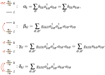 | (3) |
are the operators that encode spin-paired creation and annihilation, and the residual Hamiltonian is Hres = H − HHCB. The resulting HCB Hamiltonian, once mapped into Pauli operators, naturally decomposes into three commuting groups: {I0, Z0, Z1, Z0Z1, …}, {Y0X1X2Y3, X0Y1Y2X3, Y0X1X4Y5, …} and {Y0Y1X2X3, X0X1Y2Y3, Y0Y1X4X5, …}. Namely, αk and γkl parse into the first group, and βkl and δkl parse into the second and third groups. This makes it possible to do measurements on multiple elements at the same time, greatly reducing the computational overhead. Note that the formulation used here differs from other works20,22–24 that use a compressed representation (a single qubit for a spatial orbital) – this is, however, only possible if the quantum state is also in the HCB approximation, which is not the case here.
Since the standard measurement on quantum computers consists of reading out the classical bit values of the qubits (this corresponds to measuring in the Z-basis), we need to transform all the other Pauli operators in the Hamiltonian. This means finding a set of unitary operators such that
where
Pi(d) is a diagonal matrix in the form of a tensor product consisting only of Pauli-
Z and unit matrices. In this work, the unitary operators, or measurement circuits, were identified using the Sorted Insertion (SI) method, with an asymptotical scaling of
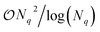
in the number of 2-qubit entangling gates and single qubit rotations.
12,25 However, in principle, they can be further optimized by tailoring them to the three groups, as the Pauli string pattern exhibits repetition.
3.2 Orbital rotation operations
An orbital basis is a unitary N × N matrix B operating on the initial set of spatial orbitals. In order to rotate a basis we need to define an operation that preserves the electronic Hamiltonian structure. An effective 2D rotation (Givens rotation) acts as a proper basis change for consecutive orbitals. Thus, in order to rotate any orbital, we can use a sequence of effective 2D rotations acting on the atomic orbital space. To illustrate, this is the matrix representation in the space of two spatial orbitals p and q:| | 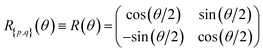 | (5) |
where θ is a free parameter. This operation is applied to the molecular integrals to define a global unitary transformation of the Hamiltonian operator. We will refer to this operation as orbital rotation.
Such an effective 2D rotation can be also represented as a quantum circuit, given the correspondence between atomic orbital space and qubit space.26–28 In fact, the unitary operator
| | 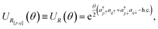 | (6) |
which acts on the qubit space, achieves the same result of an orbital rotation operation.
28 Here,
p and
q represent the spatial orbitals affected by the rotation. Thus, analogously to the atomic orbital space, an orbital rotation operation in the qubit space is achieved with a sequence of
UR(
θ). While the matrix representation is an
N ×
N operation on the space of
N spatial orbitals, the circuit representation corresponds to a 2
2N × 2
2N transformation applied on the qubit register.
4 Detailed description
The proposed method consists of four steps: a preprocessing phase (steps 1–2), performed once, a recursive phase (step 3), and a final phase (step 4), executed for each estimation of the expectation value of the whole Hamiltonian (Fig. 1).
 |
| | Fig. 1 Illustration of the measurement routine used in this article, leveraging the HCB approximation and basis rotations. The general procedure is applied to hydrogenic systems like H4 (depicted in the figure), H6 and H8. Here diagonal and off-diagonal matrix elements (green and blue) are used to represent HCB and residual Hamiltonian elements. | |
(1) Choose orbital bases  .
.
The orbital bases are given as unitary N × N matrices that operate on the initial set of orbitals, called “reference orbitals”. Note that they do not need to be “Hartree–Fock” orbitals; they merely define the reference for Bk. Each matrix in  is compiled into an orbital rotation operation forming the set
 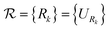 of rotation matrices and corresponding quantum circuits.
(2) Prepare the quantum state of interest.
This can be defined as
where
U is a quantum circuit, and |0〉 the quantum register. This is the state of which we aim to compute the expectation value.
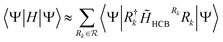
(3) Iteratively approximate the expectation value of H.
H is transformed into H = ![[H with combining tilde]](https://www.rsc.org/images/entities/i_char_0048_0303.gif) HCBR1 + H′, with
HCBR1 + H′, with
| | | HCBR1 = (R1HR†1)HCB | (8) |
An expectation value of HCBR1 can be estimated straightforwardly since all the terms can be collected into three commuting groups, as shown before. The error of this estimate is contained within the residual operator H′, which can be recursively processed in the same way we did for H. Each cycle will take a new rotation operation from the set {R1, R2, R3, …}, rotate back in the original basis, rotate forward in the new basis, and extract the HCB and residual Hamiltonian.
(4) Accumulate all contributions.
Finally, we have collected a series of expectation values that approximate the expectation value of the original Hamiltonian H.
| |  | (10) |
The expectation value over the last constructed residual operator H′ quantifies the error exactly. The approximation neglects this final residual.
The crucial point of the method is that an accurate approximation is bound to a correct choice of the orbital rotations; this is the heuristic part in step 1. In the following, we present two typical scenarios for practical applications, where we guess orbital bases based on the structure of the given electronic system and leverage concepts from valence-bond theory. We further showcase some instances with randomly selected bases.
4.1 Numerical results: measurement groups
To analyze and illustrate the method proposed above, we will consider two explicit scenarios. One uses the exact ground state and we will employ valence-bond based heuristics to generate the orbital rotations necessary in the first step of the method. In the second scenario, we will illustrate co-design with existing circuit designs to generate the orbital rotations.
Scenario I: we make no assumption on the quantum circuit that produces the state. In order to run the simulations, we computed the true ground-state through exact diagonalization. This ensures that all essential correlations are represented in the wavefunction of interest. For the rotation operations, we leverage valence-bond theory for chemical bonding construction29 following some of our previous works.21,28 For example, for a H4 molecule arranged in a linear geometry, we can define a graph identified by only paired edges, namely G1 = {{0, 1}, {2, 3}}:
Then, given a set of reference orbitals, we can associate one orbital rotation operation with each graph. In a minimal STO-3G atomic basis, G1 corresponds to a rotation in a four-orbital space. By arranging the values in rows {0, 1}, {2, 3}, corresponding to the graph nodes, the operation can be represented by the matrix (for  ):
):
| | 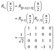 | (11) |
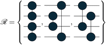
The coefficients show that the orbitals are now in an equal superposition; thus, we can interpret the first row as a bonding molecular orbital between atomic orbitals 0 and 1, the second row as an anti-bonding molecular orbital, and likewise for the third and fourth rows. Therefore, the rotation operation RG1 is the transformation from the set of reference orbitals B0, where the atomic orbitals have no interactions among them, to the orbital basis B1, where orbital pairs {0, 1}, {2, 3} are delocalized into bonding and anti-bonding motifs. The graph G1 corresponds to p, q = 0, 1 and p, q = 2, 3. We will represent such circuits graphically as
| | 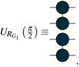 | (12) |
where the lines represent spatial orbitals (and therefore 2-qubits in most encodings). The corresponding unitary operators are:
| | 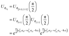 | (13) |
Scenario II: here we consider the quantum circuit design of ref. 28 explicitly and illustrate co-designing the ansatz together with the set of rotations for the measurements. This strategy enables the measurement process to adapt to the specific state produced by the quantum register. Moreover, it takes advantage of the circuit structure for the Hamiltonian evaluations. In this instance we built a quantum circuit defined by a sequence of rotations URk and double excitations: 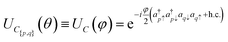 . This multi-graph circuit was defined in ref. 28.
The circuit is made of a sequence of gates that aims at catching all the correlation contributes among the atoms. In order to do that, it leverages the graph structure, i.e., the nodes of the graph define the correlated orbitals and the edges define the strength of the interaction. The produced state will be an approximation of the true wavefunction, as is typical in VQE algorithms, but we can interpret the rotation operations as existing contributions inside the quantum state, reflecting its underlying structure.
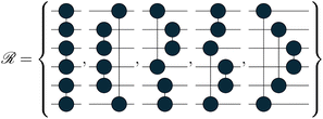
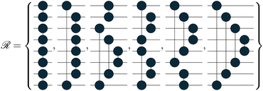
We tested the method on three molecular systems, H4, H6 and H8, all arranged both on a line, with a bond length of 1.5 Å, and scattered in space. The line configuration is a common benchmark dataset for quantum algorithms and in previous work28 they proved to be valid stand-ins for real molecular systems, such as conjugated pi-systems of carbon atoms. To broaden our analysis, we also considered free geometries that hold no structure. A bond length between the bonding and the dissociation distance makes the ground-state wavefunction not trivially simulable and not accurately representable as an HCB approximation. The sets of orbital rotation operations used are tailored to the graphs that can be defined by creating only paired connections between atoms. We defined 3, 5 and 6 graphs for the H4, H6 and H8 systems, respectively. For scattered H6 molecules, we generated 50 additional unitary transformations that were randomly generated. The corresponding quantum gates in Jordan–Wigner encoding are:
| |  | (14) |
| |  | (15) |
| |  | (16) |
using 8, 12 and 16 qubits, respectively.
The topology of the rotation operations is derived from valence-bond theory resonance structures. In particular, the number of structures available scales as  . These are the non-crossing perfect matchings of n nodes in a ring. For H4, H6 and H8 there are 2, 5 and 14 structures respectively. In the presented sets, we considered one additional structure for H4, operation number three, because the two structures alone were not able to catch all the relevant interactions in the molecule. We considered only 6 of the structures for H8, for simplicity. The number of structures one can use scales fast but the used sets have proven to be effective for the target systems. This does not prevent the use of different topologies such as crossing edges or graphs with multiple pairs as long as the operations are well defined.
Fig. 3 shows the error in the Hamiltonian approximation for each iteration. Fig. 2 shows the number of measurement groups and the depth overhead in the measuring circuits in comparison with grouping heuristics. When computing the depth of measuring circuits, the values for Scenario I and II are considered in the Reordered Jordan–Wigner encoding, meaning that the qubit order in the quantum register follows the pattern |↑↑…↑↓↓…↓〉. This choice leads us to a lower depth overhead by decoupling spin-up and spin-down excitations gates.
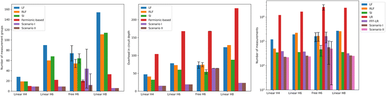 |
| | Fig. 2 (Left) Number of measurement groups needed for different reduction methods (Table 1). Free H6 refers to randomized molecular geometries, and the values correspond to the mean and standard deviation of the distribution that achieves an error below 2 mEh. (Middle) Overhead in circuit depth given by the application of a rotation operation on the wavefunction in step 4. Here we considered only linear system examples since the results are compatible. The values of Scenario I and II are expressed in the Reordered Jordan–Wigner encoding. (Right) Number of measurements required to compute all the contributions given by the general procedure. This represents the cost for each shot of a VQE algorithm. | |
Table 1 Overview over the state-of-the-art methods used for the comparison with Scenario I and II in Fig. 2, with references
| Pauli-grouping |
| Large first (LF) |
11
|
| Recursive largest first (RLF) |
11
|
| Sorted insertion (SI) |
12 and 25 |
| Fermionic-grouping |
| Low-rank decomposition (LR) |
14 and 15 |
| Fluid fermionic fragments (FFF-LR) |
16
|
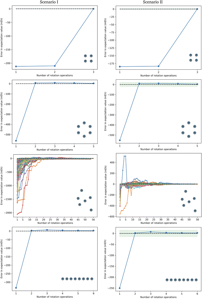 |
| | Fig. 3 Error in approximating the molecular Hamiltonian for square H4 and circular H6 as well as free H6 and linear H8 using the sets {RGk} from eqn (14)–(16), respectively. The blue area is the 1 mEh margin of error, which we consider as the desired accuracy; the green area is the error from the chosen circuit ansatz. | |
4.2 Numerical results: individual shots
Given H = ∑iHi = ∑iwiPi, for each Pauli string Pi we estimate the number of measurements as:| |  | (17) |
where ε = 10−3 represents the precision.14 Then, for each commuting group we only consider the largest value| |  | (18) |
since we can measure the operators belonging to such a group simultaneously, therefore giving an upper bound on the total measurements for the given fragment. Finally, we sum together all the contributions from each iteration to retrieve the total number of measurements.| | 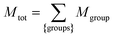 | (19) |
Fig. 2 shows the number of measurements needed for a complete repetition of the procedure compared to grouping heuristics. These values have been proven consistent from the finite sample simulations in Fig. 4. The number of samples was set to the estimated number of measurements, previously defined as the maximum value among all Pauli strings within the same group. We then repeated this process 100 times and computed the average over all sample simulations for each group. Our assumption is that the final result remains below the previously fixed precision ε = 10−3 with respect to the real expectation value. In Scenario I and II, the measurement groups are distributed and evaluated over each rotation operation, whereas for SI they are computed simultaneously. In all considered examples the error never exceeds the precision, thus confirming the consistency of the estimated number of measurements.
 |
| | Fig. 4 Finite sample simulation for three molecules: linear H4, linear H6 and linear H8. The SI method is used as a benchmark. In Scenario I and II, the rotation operations and the measured groups correspond to those used for the approximation of Hamiltonian expectation values. As mentioned above, we set a threshold precision of ε = 10−3. | |
4.3 Scientific software
All the calculations have been carried within the tequila30 Python package. Specifically, the simulations made use of qulacs31 and the qubit operator elaboration utilized OpenFermion,32 while the integral computations employed the pyscf package33 and the exact diagonalization employed scipy.34 Finally, free geometries have been generated with quanti-gin35 and circuit depictions are made with qpic.36
5 Conclusion and outlook
In all cases examined, we consistently retrieved accurate approximations for the expectation value of the molecular Hamiltonian, achieving this with a comparably small number of iterations. Moreover, compared to existing approaches, our method does not rely on extensive pre-computation. The number of measurement groups is improved by 50% to 80% compared to benchmarks.19 In Scenario II, 80% of the distribution falls under 10 measurement groups. The co-design of circuit and rotation operations may lead to more expressivity in the HCB Hamiltonian evaluation and thus fewer algorithm iterations being needed, though this is not fully conclusive yet. Orbital rotation operations have been shown to statistically improve this approximation at a cheap cost in circuit depth overhead, even when generated randomly. This work provides the basis to conduct further research to single out the optimal class of operations. Notably, the total number of measurements is lower by about 30% to 80% for structured systems, while being comparable in magnitude to benchmarks for less-structured examples. The target systems have been proved to be well described by the graph-based approach introduced.23,28 This agreement validates the efficacy of the proposed method, indicating the underlying principles are fundamental to the structural properties of these systems and supporting the hypothesis that the method can be systematically generalized to a broader range of systems. In the Appendix, we show the example of the BeH2 molecule, for which we applied the same procedure as the linear H4 molecule. The same reasoning can be applied by using circular H6 to measure the benzene molecule. Future heuristics could leverage modern correlation measures37–39 to enhance Hamiltonian approximation, or make use of perturbative methods40,41 to narrow the choice of rotation operations with respect to expressivity and efficiency.
This approach has a connection to fermionic quantum compute platforms. In ref. 42, a randomized protocol has been developed that leverages rotations into different fermionic bases – these operations are identical to the UR operations used in this work. For this reason, our heuristic protocol can be straightforwardly applied on such platforms with large improvements, e.g., the H4 system required a few thousand basis rotations while the heuristic approach from this work requires only 3 rotations. The two approaches are two goalposts, a structural approach and a randomized zero-knowledge approach,42 that can be combined. In this work, we indicated this in Fig. 3, where we used a primitive randomized protocol. One can see the randomized protocol as an upper bound, a costly brute force attempt, and the structured scheme as a lower bound, a cheap structured attempt that can mitigate the high measurement costs as soon as structural information about the system is available.
Author contributions
DB: writing (original draft), formal analysis, methodology, software, data curation, visualization. JSK: conceptualization, project administration, supervision, funding acquisition, software, writing (review and editing).
Conflicts of interest
There are no conflicts to declare.
Data availability
All data have been computed using the open-source library Tequila (v1.9.9 DOI: https://doi.org/10.5281/zenodo.7673865).30 A prototype implementation of the developed methods as well as data presented in the main text can be found under DOI: https://doi.org/10.5281/zenodo.17607750.
Supplementary information (SI) is available. See DOI: https://doi.org/10.1039/d5dd00251f.
Appendices
Close-up visualization
Fig. 6 displays close-up visualizations of the approximation figures, i.e., the errors in approximating the molecular Hamiltonian operators of the selected examples.
 |
| | Fig. 5 Quantum circuit used in Scenario II for linear H6 molecule. | |
 |
| | Fig. 6 Close-up visualization of Fig. 3. The blue area is the 1 mEh margin of error, which we consider as the desired accuracy; the green area is the error from the chosen circuit ansatz. | |
Multiple atomic distances
Fig. 7 shows the error measured for the linear H4 with respect to interatomic distance. We can see that for short distances, the chosen rotation operations behave poorly. A possible explanation for this result is that the operations defined through valence-bond theory transform the orbital basis in a localized basis. This process makes it not accurate for situations where atoms are close together, whereas a delocalized basis, e.g., canonical orbitals, can prove more suitable. This behaviour can be observed in the simulation of randomized H6 geometries, where we noticed that the original set of operations alone is not enough to retrieve the full Hamiltonian. The solution adopted in that context, i.e., adding randomly generated unitary transformations, can be transferred to this system as well, even if the resulting measurement process becomes more expensive. Note, however, that this is significantly beyond the number of orbital rotations from comparable methods applied to the same system.42
 |
| | Fig. 7 Error in approximating the molecular Hamiltonian of a linear H4 molecule. (Top) We considered multiple atomic distances and only the standard set of rotation operations for the H4 molecule. (Bottom) We considered only a 0.5 Å atomic distance and on top of the standard set we added 50 randomly generated unitaries as rotation operations, in the same manner as with H6 molecules in random geometries (Fig. 3). For further explanation see the Appendices. | |
Scenario II quantum circuit
The quantum circuit used in Scenario II is taken from ref. 28. It is made of a sequence of rotation (UR) and correlation (UC) gates. For example, the circuit used for linear H6 is| | 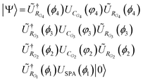 | (20) |
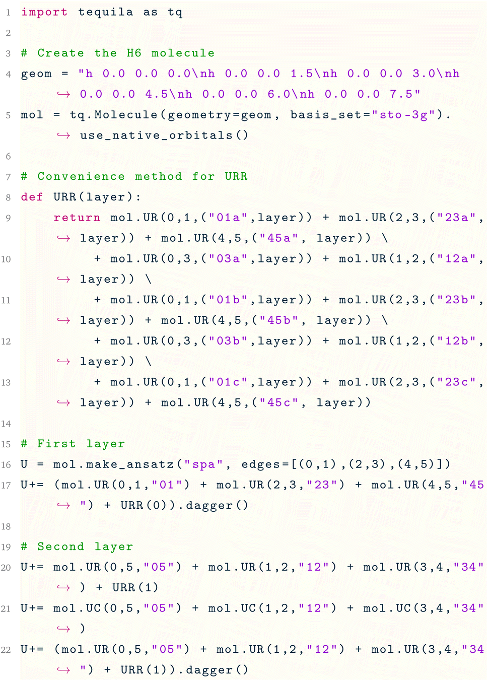
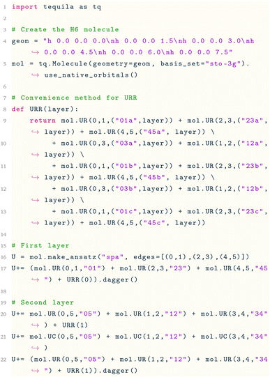
where USPA(φ1) is equivalent to 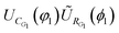 , since applying a rotation operation at the beginning of the circuit has no effect on the initial state. Fig. 5 presents the circuit rendered with qpic. In this context, ŨRk = URkURR is an extension of the orbital rotation operation that preserves the topology and allows delocalization. The definition of URR is based on eqn (20) of ref. 28. The parameters for the ŨRk gates are initialized through the GNM method from ref. 21 and then the whole is minimized. We show an example code to create the circuit for linear H6 in Fig. 1.
BeH2 molecule and method scaling
In order to assess the scaling of the method, we applied it on the BeH2 molecule. The results are shown in Fig. 8. The orbital rotation operations are the same as the linear H4 molecule and the accuracy comparably high. We didn’t consider the px and py orbitals, but only the s and pz ones. This makes it suitable for the linear H4 graph topology. The example shows how the heuristic can be extended to larger molecules by applying the same orbital rotation operations to molecules with the same topology. A similar example is the application of the operations of linear H6 over the benzene molecule. In addition, one can consider the discarded orbitals using a mixed Fermionic–Bosonic encoding24 to obtain a complete description of the system.
 |
| | Fig. 8 Error in approximating the molecular Hamiltonian of a BeH2 molecule with a bond distance of 1.5 Å in Scenario I. This shows that the heuristic can be extended to larger molecules with the same topology by applying the same orbital rotation operations. | |
Excited state calculation
The measurement protocol can be extended to excited-state calculations. In order to prove this, we considered the five lowest Hamiltonian eigenvector states with 〈S2〉 = 0 and energy higher than the ground state. The procedure is unchanged and the rotation operations are the same as those used for the ground-state computation. The result is shown in Fig. 9.
 |
| | Fig. 9 Error in approximating the molecular Hamiltonian of a linear H4 molecule for the first five excited states. (Left) Full plot. (Right) Close-up visualization. This shows that the process is not limited to computation of ground-state expectation values, but can be extended to arbitrary many-body states. | |
|
Listing 1 How to prepare a quantum circuit in tequila |
|
Acknowledgements
This work has been funded by the German Federal Ministry of Research, Technology and Space (BMFTR, Quantum Technologies: HoliQC2).
Notes and references
- A. Peruzzo, J. McClean, P. Shadbolt, M.-H. Yung, X.-Q. Zhou, P. J. Love, A. Aspuru-Guzik and J. L. O’brien, Nat. Commun., 2014, 5, 4213 CrossRef CAS PubMed.
- J. R. McClean, J. Romero, R. Babbush and A. Aspuru-Guzik, New J. Phys., 2016, 18, 023023 Search PubMed.
- J. Tilly, H. Chen, S. Cao, D. Picozzi, K. Setia, Y. Li, E. Grant, L. Wossnig, I. Rungger, G. H. Booth and J. Tennyson, Phys. Rep., 2022, 986, 1–128 Search PubMed.
- A. Anand, P. Schleich, S. Alperin-Lea, P. W. K. Jensen, S. Sim, M. Díaz-Tinoco, J. S. Kottmann, M. Degroote, A. F. Izmaylov and A. Aspuru-Guzik, Chem. Soc. Rev., 2022, 51, 1659–1684 RSC.
- K. Bharti, A. Cervera-Lierta, T. H. Kyaw, T. Haug, S. Alperin-Lea, A. Anand, M. Degroote, H. Heimonen, J. S. Kottmann, T. Menke, W.-K. Mok, S. Sim, L.-C. Kwek and A. Aspuru-Guzik, Rev. Mod. Phys., 2022, 94, 015004 CrossRef CAS.
- M. Cerezo, A. Arrasmith, R. Babbush, S. C. Benjamin, S. Endo, K. Fujii, J. R. McClean, K. Mitarai, X. Yuan, L. Cincio and P. J. Coles, Nat. Rev. Phys., 2021, 3, 625–644 CrossRef.
- P. Schleich, J. S. Kottmann and A. Aspuru-Guzik, Phys. Chem. Chem. Phys., 2022, 24, 13550–13564 RSC.
-
F. Langkabel, S. Knecht and J. S. Kottmann, The advent of fully variational quantum eigensolvers using a hybrid multiresolution approach, arXiv, 2024, preprint, arXiv:2410.19116, DOI:10.48550/arXiv.2410.19116.
- A. Aspuru-Guzik, A. D. Dutoi, P. J. Love and M. Head-Gordon, Science, 2005, 309, 1704–1707 CrossRef CAS PubMed.
- J. F. Gonthier, M. D. Radin, C. Buda, E. J. Doskocil, C. M. Abuan and J. Romero, Phys. Rev. Res., 2022, 4, 033154 CrossRef CAS.
- V. Verteletskyi, T.-C. Yen and A. F. Izmaylov, J. Chem. Phys., 2020, 152, 124114 CrossRef CAS PubMed.
- Z. P. Bansingh, T.-C. Yen, P. D. Johnson and A. F. Izmaylov, J. Phys. Chem. A, 2022, 126, 7007–7012 CrossRef CAS PubMed.
- T.-C. Yen, A. Ganeshram and A. F. Izmaylov, npj Quantum Inf., 2023, 9, 14 CrossRef PubMed.
- W. J. Huggins, J. R. McClean, N. C. Rubin, Z. Jiang, N. Wiebe, K. B. Whaley and R. Babbush, npj Quantum Inf., 2021, 7, 83 CrossRef.
- T.-C. Yen and A. F. Izmaylov, PRX Quantum, 2021, 2, 040320 CrossRef.
- S. Choi, I. Loaiza and A. F. Izmaylov, Quantum, 2023, 7, 889 Search PubMed.
- G. García-Pérez, M. A. Rossi, B. Sokolov, F. Tacchino, P. K. Barkoutsos, G. Mazzola, I. Tavernelli and S. Maniscalco, PRX Quantum, 2021, 2, 040342 CrossRef.
- D. Miller, L. E. Fischer, K. Levi, E. J. Kuehnke, I. O. Sokolov, P. K. Barkoutsos, J. Eisert and I. Tavernelli, npj Quantum Inf., 2024, 10, 122 CrossRef PubMed.
-
A. Gresch, U. Tepe and M. Kliesch, arXiv, 2025, preprint, arXiv:2502.01730, DOI:10.48550/arXiv.2502.01730.
- V. E. Elfving, M. Millaruelo, J. A. Gámez and C. Gogolin, Physical Review A: Atomic, Molecular, and Optical, Physics, 2021, 103, 032605 CAS.
- J. S. Kottmann and F. Scala, J. Chem. Theory Comput., 2024, 20, 3514–3523 CrossRef CAS PubMed.
- L. Zhao, J. Goings, K. Shin, W. Kyoung, J. I. Fuks, J.-K. K. Rhee, Y. M. Rhee, K. Wright, J. Nguyen, J. Kim and S. Johri, npj Quantum Inf., 2023, 9, 60 CrossRef.
- J. S. Kottmann and A. Aspuru-Guzik, Phys. Rev. A, 2022, 105, 032449 CrossRef CAS.
- F. J. del Arco Santos and J. S. Kottmann, Quantum Sci. Technol., 2025, 10, 035018 CrossRef.
-
O. Crawford, B. van Straaten, D. Wang, T. Parks, E. Campbell and S. Brierley, arXiv, 2019, preprint, arXiv:1908.06942, DOI:10.48550/arXiv.1908.06942.
- I. D. Kivlichan, J. McClean, N. Wiebe, C. Gidney, A. Aspuru-Guzik, G. K.-L. Chan and R. Babbush, Phys. Rev. Lett., 2018, 120, 110501 CrossRef CAS PubMed.
- Google AI Quantum and Collaborators, Science, 2020, 369, 1084–1089 CrossRef PubMed.
- J. S. Kottmann, Quantum, 2023, 7, 1073 CrossRef.
-
S. Shaik, P. C. Hiberty, A Chemist’s Guide to Valence Bond Theory, John Wiley & Sons, Ltd, 2007, ch. 9, pp. 238–270 Search PubMed.
- J. S. Kottmann, S. Alperin-Lea, T. Tamayo-Mendoza, A. Cervera-Lierta, C. Lavigne, T.-C. Yen, V. Verteletskyi, P. Schleich, A. Anand, M. Degroote, S. Chaney, M. Kesibi, N. G. Curnow, B. Solo, G. Tsilimigkounakis, C. Zendejas-Morales, A. F. Izmaylov and A. Aspuru-Guzik, Quantum Sci. Technol., 2021, 6, 024009 CrossRef.
- Y. Suzuki, Y. Kawase, Y. Masumura, Y. Hiraga, M. Nakadai, J. Chen, K. M. Nakanishi, K. Mitarai, R. Imai, S. Tamiya, T. Yamamoto, T. Yan, T. Kawakubo, Y. O. Nakagawa, Y. Ibe, Y. Zhang, H. Yamashita, H. Yoshimura, A. Hayashi and K. Fujii, Quantum, 2021, 5, 559 CrossRef.
- J. R. McClean, N. C. Rubin, K. J. Sung, I. D. Kivlichan, X. Bonet-Monroig, Y. Cao, C. Dai, E. S. Fried, C. Gidney, B. Gimby, P. Gokhale, T. Häner, T. Hardikar, V. Havlíček, O. Higgott, C. Huang, J. Izaac, Z. Jiang, X. Liu, S. McArdle, M. Neeley, T. O’Brien, B. O’Gorman, I. Ozfidan, M. D. Radin, J. Romero, N. P. D. Sawaya, B. Senjean, K. Setia, S. Sim, D. S. Steiger, M. Steudtner, Q. Sun, W. Sun, D. Wang, F. Zhang and R. Babbush, Quantum Sci. Technol., 2020, 5, 034014 CrossRef.
- Q. Sun, T. C. Berkelbach, N. S. Blunt, G. H. Booth, S. Guo, Z. Li, J. Liu, J. D. McClain, E. R. Sayfutyarova, S. Sharma, S. Wouters and G. K.-L. Chan, Wiley Interdiscip. Rev. Comput. Mol. Sci., 2018, 8, e1340 CrossRef.
- P. Virtanen, R. Gommers, T. E. Oliphant, M. Haberland, T. Reddy, D. Cournapeau, E. Burovski, P. Peterson, W. Weckesser, J. Bright, S. J. van der Walt, M. Brett, J. Wilson, K. Jarrod Millman, N. Mayorov, A. R. J. Nelson, E. Jones, R. Kern, E. Larson, C. J. Carey, İ. Polat, Y. Feng, E. W. Moore, J. Vand erPlas, D. Laxalde, J. Perktold, R. Cimrman, I. Henriksen, E. A. Quintero, C. R. Harris, A. M. Archibald, A. H. Ribeiro, F. Pedregosa, P. van Mulbregt and S. 1.0 Contributors, Nat. Methods, 2020, 17, 261–272 CrossRef CAS PubMed.
-
K. Stein, Nylser/Quanti-Gin, 2024, https://github.com/nylser/quanti-gin Search PubMed.
-
T. G. Draper and S. A. Kutin, Qpic/Qpic, qpic, 2025, https://github.com/qpic Search PubMed.
- L. Ding, S. Mardazad, S. Das, S. Szalay, U. Schollwöck, Z. Zimborás and C. Schilling, J. Chem. Theory Comput., 2021, 17, 79–95 CrossRef CAS PubMed.
- L. Ding, S. Knecht, Z. Zimborás and C. Schilling, Quantum Sci. Technol., 2022, 8, 015015 CrossRef.
- L. Ding, S. Knecht and C. Schilling, J. Phys. Chem. Lett., 2023, 14, 11022–11029 CrossRef CAS PubMed.
-
L. Reascos, G. F. Diotallevi and M. Benito, arXiv, 2024, preprint, arXiv:2411.11535, DOI:10.48550/arXiv.2411.11535.
-
G. F. Diotallevi, L. Reascos and M. Benito, arXiv, 2024, preprint, arXiv:2412.10240, DOI:10.48550/arXiv.2412.10240.
- P. Naldesi, A. Elben, A. Minguzzi, D. Clément, P. Zoller and B. Vermersch, Phys. Rev. Lett., 2023, 131, 060601 CrossRef CAS PubMed.
|
| This journal is © The Royal Society of Chemistry 2026 |
Click here to see how this site uses Cookies. View our privacy policy here. 
 Open Access Article
 This Open Access Article is licensed under a
  a and
Jakob S.
Kottmann
a and
Jakob S.
Kottmann

 types of individual shots have to be realized in order to estimate the full expectation value. On noisy hardware, but also with respect to estimated runtimes, this overhead is currently preventing practical demonstrations of VQEs on moderate-sized systems.9,10 A class of strategies to resolve this dilemma are so-called grouping methods that identify commuting cliques in the individual parts of the Hamiltonian, which can then be measured simultaneously – therefore reducing the overhead from
  to the number of commuting cliques. As finding the optimal cliques is an NP-hard problem, various heuristics based on qubit11–13 and fermionic14–16 representations have been proposed. So far, these methods focus on (near-)exact decompositions of the full Hamiltonian without taking advantage of physical approximations tailored to the system of interest. Furthermore, there are other methods that consider adaptive procedures.17–19
 overhead described above can be eliminated by approximating the electronic system as a collection of spin-paired quasi-particles, called Hard-Core Bosons (HCBs).20 This approximation allows the Hamiltonian to be divided into exactly three commuting groups, regardless of the system size. However, this approach often falls short in accurately describing electronic systems, particularly those where quantum computers are expected to provide significant improvements in precision. Therefore, limiting variational algorithms to HCB Hamiltonians is not a viable solution. The core idea of this research is to leverage the straightforward grouping of HCB Hamiltonians and combine them with orbital rotations to switch between different frames of the approximation in order to iteratively improve the estimate of the expectation values at hand. At this point, it is important to note that the electronic states of interest are not formulated using the HCB approximation.


 in the number of 2-qubit entangling gates and single qubit rotations.12,25 However, in principle, they can be further optimized by tailoring them to the three groups, as the Pauli string pattern exhibits repetition.


 .
. is compiled into an orbital rotation operation forming the set
  of rotation matrices and corresponding quantum circuits.

 ):
):


 . This multi-graph circuit was defined in ref. 28.


 . These are the non-crossing perfect matchings of n nodes in a ring. For H4, H6 and H8 there are 2, 5 and 14 structures respectively. In the presented sets, we considered one additional structure for H4, operation number three, because the two structures alone were not able to catch all the relevant interactions in the molecule. We considered only 6 of the structures for H8, for simplicity. The number of structures one can use scales fast but the used sets have proven to be effective for the target systems. This does not prevent the use of different topologies such as crossing edges or graphs with multiple pairs as long as the operations are well defined.


 , since applying a rotation operation at the beginning of the circuit has no effect on the initial state. Fig. 5 presents the circuit rendered with qpic. In this context, ŨRk = URkURR is an extension of the orbital rotation operation that preserves the topology and allows delocalization. The definition of URR is based on eqn (20) of ref. 28. The parameters for the ŨRk gates are initialized through the GNM method from ref. 21 and then the whole is minimized. We show an example code to create the circuit for linear H6 in Fig. 1.