DOI:
10.1039/D4CS00695J
(Tutorial Review)
Chem. Soc. Rev., 2026,
55, 3737-3765
Shedding light on overpotentials and underpotentials in (photo)electrochemical reactions
Received
18th April 2025
First published on 19th February 2026
Abstract
The concept of overpotential is central to evaluating the performance of catalysts for electrochemical and photoelectrochemical transformations. This thermodynamic metric is well defined in the context of electrochemical reactions involving conducting electrodes, where the overpotential is the difference between an applied bias potential (which sets the energetics/potential of the electrode's Fermi level) and the equilibrium potential (which is set by the mixture of oxidized and reduced chemical species in the bulk solution and establishes the applied bias potential at which no net current flows, i.e., the open-circuit potential). Nonetheless, there are at least two ways the term overpotential—or in some cases “underpotential”—has been used to describe photoelectrochemical reactions involving semiconducting electrodes, where illumination results in a splitting of the photoelectrode's Fermi level into majority- and minority-carrier quasi-Fermi levels. In one approach, the overpotential/underpotential remains defined as the difference between an applied bias potential and the equilibrium potential. In the alternative approach, the overpotential is defined as the difference between the minority-carrier quasi-Fermi-level potential at the semiconductor surface and the equilibrium potential, thereby accounting for the surface photovoltage generated upon illumination of a semiconductor electrode. This article provides an overview of conceptual differences involving overpotentials and underpotentials in (photo)electrochemical reactions and considers applied electrode potentials in terms of their enthalpic versus entropic contributions.

Daiki Nishiori
| Daiki Nishiori received his PhD at Arizona State University in 2024 under the supervision of Prof. Gary F. Moore. His doctoral research focused on the use of extended electronic conjugation of molecular electrocatalysts as a strategy to break the molecular scaling relationship. He also investigated photoelectrosynthetic assemblies consisting of metalloporphyrin hydrogen-evolution catalysts immobilized on gallium phosphide semiconductors. He received his BSc and MSc in chemistry from the University of Tokyo in 2018, working with Prof. Hiroshi Nishihara. |

Edgar A. Reyes Cruz
| Edgar A. Reyes Cruz received his PhD at Arizona State University in 2023 under the supervision of Prof. Gary F. Moore. His doctoral research focused on the synthesis and characterization of catalysts for carbon dioxide reduction, and the electrochemical characterization of benzimidazole-phenols as “proton wires”. He earned his BSc in Chemistry from the Monterrey Institute of Technology and Higher Education in 2014, working with Prof. Ernesto Mariño-Ochoa. |

Lillian K. Hensleigh
| Lillian K. Hensleigh is a PhD candidate at Arizona State University, where she conducts research under the mentorship of Professor Gary Moore. She earned dual Bachelor of Science degrees in Biology and Chemistry from the University of Redlands. Her research centers on understanding structure–function relationships in heterogeneous catalytic systems, in which catalysts are immobilized onto (semi)conductive surfaces via polymeric supports, and homogeneous catalytic system where catalysts are dissolved in solution. These fundamental investigations target mechanistic insight into catalytic processes that underpin sustainable energy technologies, with the broader goal of advancing strategies for solar-to-fuels conversion and renewable energy storage. |

Nghi P. Nguyen
| Nghi Nguyen received her PhD at Arizona State University in 2023 under the supervision of Prof. Gary F. Moore. Her doctoral research focused on surface modification of III–V semiconductors with molecular catalysts embedded in thin-film polymeric coating. The coordination of earth-abundant metal centers within the three-dimensional molecular coatings allows modulating the electronic and catalytic properties of the overall assembly, providing a strategy for studying the effects of polymeric-encapsulation on electrocatalytic as well as photoelectrosynthetic performance of these hybrid constructs. She received her BSc in Chemistry from University of Science, Ho Chi Minh City. |

Gary F. Moore
| Gary F. Moore is an Associate Professor in the School of Molecular Sciences at Arizona State University (ASU). He received his PhD from ASU under Ana L. Moore in 2009. And then spent two years as a Camille and Henry Dreyfus Energy Fellow at Yale University, working with Gary W. Brudvig and Robert H. Crabtree. He started his independent research career at Berkeley Lab in 2011 and moved to ASU in 2014. Moore is a Presidential Early Career Awardee, a National Academy of Sciences Kavli Foundation Fellow, a Camille Dreyfus Teacher-Scholar Awardee, a Department of Energy Early Career Awardee, and a National Science Foundation CAREER Awardee. |
Key learning points
(1) Defining overpotentials in electrochemistry
(2) Defining overpotentials in electrocatalysis
(3) Defining overpotentials versus underpotentials in semiconductor photoelectrochemistry
(4) Defining overpotentials versus underpotentials in catalyst-modified semiconductor photoelectrochemsitry
(5) Differentiating the enthalpic versus entropic components of applied electrode potentials
|
I. Introduction and context
Replacing fossil-based energy sources with environmentally sustainable alternatives has spurred interest in electrochemical and photoelectrochemical approaches to generating fuels and other value-added chemical products.1,2 Strategies for achieving this transition range from indirect approaches that use electricity produced from renewable sources (e.g., wind or solar) to power fuel-forming reactions at physically separated electrocatalytic units, to more integrated approaches that use a single photoelectrochemical device to capture, convert, and store the sun's energy as fuels (Fig. 1). In general, the more indirect approaches have a higher technological readiness level (TRL), and the required components are often commercially available. Conversely, the more integrated approaches have a lower TRL but are active areas of research given their promise to use fewer material components and lower operating costs.
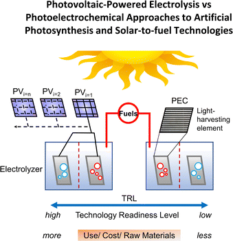 |
| | Fig. 1 A diagram depicting varying approaches to achieving solar-to-fuel technologies, including those at a relatively high technology readiness level (TRL) (far left and illustrated as a photovoltaic-powered electrolysis device driving an overall energetically “uphill” reaction to produce fuels) and those at a relatively low TRL (far right and depicted as a photoelectrochemical device that uses catalyst-modified semiconductors). Tradeoffs between current use, projected costs, and consumption of raw materials across the TRL spectrum are also indicated. Adapted with permission from Ardo et al., 2018. Copyright 2018 The Royal Society of Chemistry. | |
Light harvesting is a commonality among the varying approaches indicated in Fig. 1, but is only the upfront step. Large-scale deployment of renewable energy sources requires energy storage.3,4 For this reason, catalysts are essential to artificial photosynthesis and solar-to-fuel technologies, as they provide relatively lower energetic pathways for storing energy in the form of chemical bonds. In this article, we review established and emerging approaches to benchmarking the performance of electrocatalytic and photoelectrosynthetic assemblies, where the latter utilize light to drive thermodynamically uphill reactions. Emphasis is placed on the role of overpotentials and underpotentials in controlling the rates of electrochemical and photoelectrochemical reactions.
II. Overpotentials in electrochemistry
A. Overview of electrochemistry and electrochemical potentials
Electrochemistry is a branch of chemistry concerning the interrelation of electrical and chemical effects, including chemical changes induced by the passage of current and the production of electrical energy by chemical reactions.5 The reactivity, transport, and transfer of both charged and uncharged species are all driven by differences in electrochemical potential (![[small mu, Greek, macron]](https://www.rsc.org/images/entities/i_char_e0cd.gif) αj, with units of J mol−1 and defined as the partial molar Gibbs free energy of a given species j in phase α).5–7 Examples include differences in the electrochemical potential of electrons in metals (me) that drive charge flow, as well as spatial gradients in the electrochemical potential of oxidized (Ox) and reduced (Red) chemical species in a solution (solOx and solRed, respectively) that drive mass transport. Electrochemical potentials can be deconvoluted into contributions from a chemical component and an electric component, as indicated in eqn (1),5,6
αj, with units of J mol−1 and defined as the partial molar Gibbs free energy of a given species j in phase α).5–7 Examples include differences in the electrochemical potential of electrons in metals (me) that drive charge flow, as well as spatial gradients in the electrochemical potential of oxidized (Ox) and reduced (Red) chemical species in a solution (solOx and solRed, respectively) that drive mass transport. Electrochemical potentials can be deconvoluted into contributions from a chemical component and an electric component, as indicated in eqn (1),5,6
| | | (the electrochemical potential of a species j in phase α), | (1) |
where μαj is the chemical potential of a species j in phase α, zj is the sign charge number of the species, F is the Faraday constant, and ϕα is the electric potential in phase α. In the following Sections B and C, we describe these components in further detail and introduce other relevant physical quantities.
B. The chemical component of electrochemical potentials
The chemical component of an electrochemical potential [see eqn (1)] is the chemical potential of a speciesjin phaseα (μαj, with units of J mol−1). As indicated in eqn (2), μαj, is the partial derivative of the chemical free energy of a species j in phase α (G, with units of J and defined as the Gibbs free energy of a species j in phase α excluding electrostatic contributions due to uncompensated charges) with respect to the number of moles of a speciesj (nj, with units of mol), while keeping the absolute temperature (T, with units of K), pressure (P, with units of Pa), and number of moles of all other species aside fromj (ni≠j, with units of mol) constant,5| |  | (2) |
Thus, μαj is a partial molar quantity representing the change in Gibbs free energy of phase α when one mole of j is added to phase α while keeping the values of T, P, and ni≠j unchanged. By extension, and as further indicated in eqn (2), μαj can also be expressed in terms of the standard chemical potential of a speciesjin phaseα [ with units of J mol−1 and defined as the chemical potential of the species j in phase α in the standard state (i.e., the state of a system chosen as a standard for reference by convention8)], the universal gas constant (R, which is exactly 8.31447261815324 J K−1 mol−1), and the chemical activity of a speciesjin phaseα (aαj, a dimensionless quantity defined as the thermodynamic concentration accounting for non-ideal behavior arising from intermolecular interactions between all species present in the solution).9,10
For a gas, the standard state is the hypothetical state of the pure substance in the gaseous phase at the standard pressure (p°, with units of Pa and defined as the chosen value of pressure as a standard for reference), assuming ideal behavior.8 For a liquid or solid, the standard state is the state of the pure substance in the liquid or solid phase, respectively, at the standard pressure. For a solute in solution, the standard state is the hypothetical state of the solute at the standard molality (m°, with units of mol kg−1 and defined as moles of solute per unit mass of the solvent selected as a standard for reference), standard pressure, or standard concentration (c°, with units of mol cm−3 and defined as moles of a solute per unit volume of the solution selected as a standard for reference) and exhibiting “infinitely dilute solution behavior”. Although not universally accepted, commonly used standards established by the International Union of Pure and Applied Chemistry (IUPAC) include p°, m°, and c°, which are defined as 105 Pa, 1 mol kg−1, and 1 mol L−1 (= 10−3 mol cm−3), respectively.8 The term standard state differs from the term standard temperature and pressure (STP), which IUPAC defines as a temperature of 273.15 K (0 °C) and pressure of 105 Pa.8
For solution phases, the chemical activity coefficient of a speciesjin the solution phase (γsolj, a dimensionless quantity that is the ratio of the chemical activity to the molar concentration) accounts for deviations from ideal behavior.9 The chemical activity of a species j in the solution phase, asolj, can thus be expressed as a product of γsolj and the concentration of a speciesjin the solution phase (Csolj, with units of mol L−1 and defined as moles of a species j as a solute per unit volume of the solution) divided by the standard concentration, c°, as expressed in eqn (3),2
| |  | (3) |
When the amount of a species
j in phase
α is relatively low, meaning
γsolj is close to unity, their chemical activities can be approximated by their concentrations.
9,11
For gas phases, the fugacity of a speciesjin the gas phase (fgasj, with units of Pa and defined as the pressure of an ideal gas that has the same molar Gibbs free energy as the real gas j at the same temperature)12 accounts for the non-ideal behavior of a gas.13,14 As indicated in eqn (4), the chemical activity of a species j in the gas phase, agasj, is given by the ratio of fgasj to the standard pressure, p°.15 Further, agasj can be related to the ratio pj and p° by the fugacity coefficient14,16 (ϕj, a dimensionless quantity defined as the ratio of the fugacity of a species j to the partial pressure of the species j in phase α), which is analogous to γsolj but accounts for deviations from an ideal gas instead of an ideal solution,
| |  | (4) |
C. The electric component of electrochemical potentials
The electric component of an electrochemical potential [see eqn (1)] arises from electrostatic interactions between charged species. The magnitude of charge associated with a single electron or proton is the elementary charge (e, which is defined as exactly 1.602176634 × 10⁻¹⁹ C).8 Congruently, the unit charge (which is 1 C) is defined as the amount of charge per second traversing a given point in a circuit when the current is 1 A.8Coulomb's inverse-square law, indicated in equation eqn (5), yields the resulting electrostatic force (![[F with combining right harpoon above (vector)]](https://www.rsc.org/images/entities/i_char_0046_20d1.gif) electrostatic, with units of N and defined as a vector quantity that is the time derivative of momentum and the attractive or repulsive force between two electrically charged objects)8 that a test charge (q, with units of C and defined as the hypothetical charge located at a single point in space that has a negligible effect on the charge distribution around the point) experiences in the presence of a point charge (Q, with units of C and defined as a hypothetical charge located at a single point in space),
electrostatic, with units of N and defined as a vector quantity that is the time derivative of momentum and the attractive or repulsive force between two electrically charged objects)8 that a test charge (q, with units of C and defined as the hypothetical charge located at a single point in space that has a negligible effect on the charge distribution around the point) experiences in the presence of a point charge (Q, with units of C and defined as a hypothetical charge located at a single point in space),| |  | (5) |
In eqn (5), ε0 is the permittivity of vacuum [which is approximately 8.854188 × 10⁻¹² C2 N−1 m−2 and is a fundamental constant relating the speed of light in a vacuum (c, which is exactly 2.99792458 × 10⁸ m s−1) and the permeability of vacuum (μ0, which is approximately 1.256637 × 10⁻⁶ N A−2 and defined as the magnetic induction in vacuum, with units of tesla, divided by the magnetic field strength in vacuum, with units of A m−1)],8r is the distance (with units of m) between the point charge and the test charge, and ![[r with combining circumflex]](https://www.rsc.org/images/entities/i_char_0072_0302.gif) is the unit vector (with units of m and defined as a vector with length of 1) directed from the point charge to the test charge. The region surrounding a charge that exerts an electrostatic force on any other charge is the electric field (with units of V m−1, yet commonly reported with units of V cm−1).9 As shown in eqn (6), the strength and direction of the electric field created by Q are described by the electric field intensity (
is the unit vector (with units of m and defined as a vector with length of 1) directed from the point charge to the test charge. The region surrounding a charge that exerts an electrostatic force on any other charge is the electric field (with units of V m−1, yet commonly reported with units of V cm−1).9 As shown in eqn (6), the strength and direction of the electric field created by Q are described by the electric field intensity (![[E with combining right harpoon above (vector)]](https://www.rsc.org/images/entities/i_char_0045_20d1.gif) , a vector quantity with units of V m−1, yet commonly reported with units of V cm−1, and defined as the electrostatic force exerted at any point in space on a unit charge),9
, a vector quantity with units of V m−1, yet commonly reported with units of V cm−1, and defined as the electrostatic force exerted at any point in space on a unit charge),9| |  | (6) |
Leveraging the definition of the electric field intensity, , the electric component of an electrochemical potential is thus the product of the signed charge number of a speciesj (zj, which is a dimensionless quantity and defined as the ratio of the charge of j to the elementary charge, e), the Faraday constant (F, which is the magnitude of charge of one mole of elementary charge and is exactly 9.64853321233100184 × 10⁴ C mol−1), and the electric potential in phaseα (ϕα, with units of V and defined as the electric component of the work required to move a unit charge in the presence of an electric field from an infinite distance to a specified position and without crossing material interfaces) [see eqn (1)].5,6 As indicated in eqn (7), ϕα is the line integral of ,| |  | (7) |
where  represents the integral of the dot product of the electric field intensity, , and an infinitesimal displacement of a unit charge, d
![[l with combining right harpoon above (vector)]](https://www.rsc.org/images/entities/i_char_006c_20d1.gif) , along an arbitrary “path” from an infinite distance to a specified position within phase α.
, along an arbitrary “path” from an infinite distance to a specified position within phase α.
In the following Section D, we describe how electrochemical potentials are manifested in electrochemical cell configurations and expressed as electrode potentials.
D. Cell configurations and electrode potentials in electrochemistry
A common cell configuration used for electrochemical measurements involves the application of three electrodes—including a working electrode, a counter electrode, and a reference electrode—in contact with an electrolyte solution containing oxidized and reduced forms of a chemical species. Here, the electrochemical potential of electrons in phaseα [αe, with units of J mol−1 and defined as the average energy of available (i.e., transferable) electrons in phase α] is equivalent to and thus sometimes referred to as the Fermi level in phaseα (where α could be a working electrode, a counter electrode, a reference electrode, an electrolyte solution, or some other indicated phase).5 The three-electrode configuration enables the electrochemical potential of electrons in the working electrode (wee) to be thermodynamically defined and set with respect to the electrochemical potential of electrons in the reference electrode (refe) while the net current flowing between the working and counter electrodes is measured, and can yield information on the kinetics of the electrochemical reactions occurring at the working electrode|electrolyte solution interface. Given no electrical current passes between the working and reference electrodes, the Fermi level of the reference electrode, refe, remains constant with respect to a standard reference state.17 By convention, the standard reference state is the standard hydrogen electrode (SHE, defined as a hypothetical reference electrode for protic solvents, consisting of a platinized Pt electrode in an acidic solution with unit activity of protons and hydrogen gas supplied at a fugacity of 1.00 bar).8,18,19 Utilizing this arbitrary and hypothetical set of conditions pertaining to the SHE as the standard reference state, the difference between the electrochemical potential of H2 in the solution phase  and the electrochemical potential of H+ in the solution phase
  is set to zero. Thus, a Pt electrode in equilibrium (i.e., where the rates of forward and reverse reactions are equal and no net reaction takes place) with H2 and H+ at unit activities would have an electrochemical potential of electrons in platinum (Pte) equal to zero. The normal hydrogen electrode (NHE) is another type of reference electrode consisting of a Pt electrode submerged in an acidic solution, where the normality (N, with units of eq L−1 and defined as the gram equivalent weight of solute per liter of solution) of the solution is unity and hydrogen gas is supplied at a pressure of 1 atmosphere (which is equivalent to exactly 1.01325 × 10⁵ Pa).8,20 Unlike the SHE, which is a hypothetical reference electrode—because finite concentration and ideal behaviour are mutually exclusive (vide supra)—the NHE can be physically fabricated. Despite these differences, the terms NHE and SHE have sometimes been used interchangeably, so caution is advised.17
In this article, and as indicated in eqn (8), we use the term Fermi-level potential (EF, with units of V vs. a defined reference state and sometimes referred to as the electrode potential)21,22 to indicate the difference between the electrochemical potential of electrons in phase α, αe, and the electrochemical potential of electrons in a defined reference state, refe, per charge of one mole of electrons,
| |  | (8) |
The generic concept of a Fermi-level potential is extended to the
Fermi-level potential of a reference electrode (
Eref, with units of V
vs. a defined reference state), which is the Gibbs free energy change per elementary charge to move an electron from the indicated reference state to the reference electrode. Analogous to the definition of
Eref, and as expressed in
eqn (9), the
Fermi-level potential of a working electrode (
Ewe, with units of V
vs. a defined reference state) is the difference between the electrochemical potential of electrons in the working electrode,
wee, and
refe per charge of one mole of electrons,
6| |  | (9) |
Ewe can be biased using an
applied electrode potential (
Eapp, with units of V) set
via an external source (
e.g., a potentiostat) and relative to a defined reference electrode potential (
i.e.,
Eref).
8
In a three-electrode configuration, the electrode potential difference between the working and counter electrodes ramps to a value required to sustain the kinetics of the electrochemical reaction occurring at the working electrode at a rate dictated by Eapp. In most voltammograms, Eapp is represented on the x-axis, and the y-axis indicates the current flowing between the working and counter electrodes.
In a two-electrode configuration, the counter electrode is also the reference electrode. Thus, in two-electrode configurations, the rates of an overall electrochemical reaction can be limited by kinetics associated with the electrochemical reactions occurring at either the working or counter/reference electrodes.
In general, electrochemical cells are combinations of half-cells, where each half-cell is represented by a half-reaction written as a reduction [eqn (10a)] or oxidation [eqn (10b)],
| | | Ox + ne− ⇄ Red (generic reduction half-reaction), | (10a) |
| | | Red ⇄ Ox + ne− (generic oxidation half-reaction). | (10b) |
Using this convention, an
anode is defined as an electrode at which net oxidation occurs (
e.g., net electrons are transferred to the anode from a reduced species in a solution phase to drive an anodic half-reaction), and a
cathode is defined as an electrode at which net reduction occurs (
e.g., net electrons are transferred from the cathode to an oxidized species in a solution phase to drive a cathodic half-reaction).
5
The cell potential (Ecell, with units of V and defined as the difference in the Fermi-level potentials of an anode and a cathode)23 is equated to the Gibbs free energy change (ΔG, with units of J mol−1 and defined as the maximal electrical work that can be obtained from a closed system at constant temperature and pressure)12via the Faraday constant, F, and the number of moles of electrons transferred in the balanced oxidation–reduction reaction (i.e., a redox reaction) of an electrochemical cell, n, as shown in eqn (11),5,8
| |  | (11) |
where
EOx/Red (with units of V
vs. a defined reference state) is the electrode potential of a half-reaction written as a reduction by convention.
5,8,22 For an overall redox reaction that is spontaneous (
i.e., Δ
G < 0), when both half reactions are expressed as reduction reactions (by convention), the half-cell with the more positive value of
EOx/Red establishes the cathode (because it has the greater tendency to be reduced) whereas the half-cell with the more negative value of
EOx/Red establishes the anode (because it has the greater tendency to be oxidized). The value of
EOx/Red associated with a half-cell can also be expressed in terms of the
standard electrode potential of a half-reaction (

, with units of V
vs. a defined reference state and defined as the electrode potential of a half-reaction under standard conditions), as expressed in
eqn (12),
5,8,24,25| |  | (12) |
where
n is the number of electrons required to convert one molecule of Ox to one molecule of Red, and
aαOx and
aαRed are activities of Ox and Red in phase
α.
Eqn (11) and (12) are the Nernst equations for a full-cell and half-cell, respectively, yielding chemical thermodynamic relationships for calculating cell potentials or electrode potentials of a half-reaction.
5,26 Under open-circuit conditions (
i.e., where no net current flows through the cell), the value of
Ecell is equivalent to the electromotive force (EMF, with units of V), which is not a type of force but is the electric potential difference between the cathode and anode when no current is drawn from the electrochemical cell.
8
Application of the Nernst equation for a half-reaction [eqn (13)] to the proton reduction half-reaction (i.e., 2H+ + 2e− ⇄ H2) yields the Fermi-level potential of the reversible hydrogen electrode [RHE, defined as a reference electrode for protic solvents consisting of a platinized Pt electrode in an acidic solution under 1 atm (101![[thin space (1/6-em)]](https://www.rsc.org/images/entities/char_2009.gif) 325 Pa)8 of hydrogen, where the activity of H+ in the solution phase
325 Pa)8 of hydrogen, where the activity of H+ in the solution phase  or the fugacity of H2 in the gas phase
  is not required to be at standard conditions]. The reversible hydrogen electrode potential (ERHE, with units of V vs. Eref and defined as the Fermi-level potential of the reversible hydrogen electrode) is equated to the standard hydrogen electrode potential (ESHE, with units of V vs. Eref and defined as the standard electrode potential for the proton reduction half-reaction) via the Nernst relationship, as shown in eqn (13),18
| |  | (13) |
The RHE reference scale is useful because it accounts for changes in the
solution potential for hydrogen [abbreviated as pH and defined as a logarithmic scale that indicates the concentration of hydrogen ions (
i.e., H
+)] arising from changes in proton activity

. The pH of a solution is expressed as a function of

, as indicated in
eqn (14),
| |  | (14) |
Because activity coefficients are often unknown, it can be pragmatic to use the
formal potential (

, with units of V
vs. Eref and defined as the reduction potential of the half-reaction when the oxidized and reduced forms of chemical species, Ox and Red, respectively, are present in the solution phase at concentrations such that the ratio,
CsolOx/
CsolRed, is unity, but other substances—such as protons or other specified species—can be present at designated, non-standard conditions).
5 Formal potentials are expressed using the chemical activity coefficients of Ox and Red in the solution phase (
γsolOx and
γsolRed, respectively), as indicated in
eqn (15),
| |  | (15) |
When the Fermi level of a working electrode is equilibrated with the Fermi level of a solution phase (
i.e.,
EF is constant across the working electrode and solution phases), the sum of
αj for the products (Red) is equal to that of reactants (Ox + ne
−). These conditions yield a definition for the electrochemical potential of electrons in the solution phase (
sole) in terms of the electrochemical potential of Ox and Red in the solution phase (
solOx and
solRed, respectively), as shown in
eqn (16) and given that under equilibrium conditions
solOx +
nsole =
solRed,
| |  | (16) |
In a related vein, the
solution potential (
Esol, with units of V
vs. Eref and defined as the Gibbs free energy change per elementary charge to move an electron from an arbitrary reference state to the solution phase
via reduction or oxidation reactions, and accounting for any associated ion/solvent rearrangement) is set by the standard electrode potential for the half-reaction,

, and the chemical activities of Ox and Red in the solution phase (
asolOx and
asolRed, respectively), as expressed in the modified Nernst equation (including the addition of the
ϕsol and
ϕref terms) shown in
eqn (17),
6,27–29| |  | (17) |
where
ϕsol is the electric potential in the solution phase,
30 and
ϕref is the electric potential in the reference electrode. The electric potential terms,
ϕsol and
ϕref, cancel out when
Esol is measured
versus a reference electrode at the same electric potential in the solution phase.
Per the Nernst equation, and in conjunction with open-circuit conditions, the activities of Ox and Red in the bulk solution ( and
and  , respectively) set the equilibrium potential (Eeq, with units of V vs. Eref and defined as the Fermi-level potential of the solution phase determined from an applied electrode potential at which no net current flows). Thus, Eeq is equivalent in value to the open-circuit potential (Eoc, with units of V vs. Eref) established by the solution mixture when both Ox and Red are present in the solution phase and there are no contributions from liquid junctions.5,31,32 This relationship is expressed in eqn (18),
| | 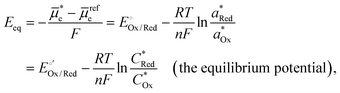 | (18) |
where

is the electrochemical potential of electrons in the bulk solution,

and

are concentrations of Ox and Red in the bulk solution. Unlike
Esol (which can be position-dependent with respect to the distance from the electrode surface and is defined by the position-dependent
asolOx and
asolRed),
Eeq is defined under equilibrium conditions and thus is not position-dependent.
6,33 Nonetheless, at equilibrium (
i.e., where
αj for all species is constant with position)
Esol is equal to
Eeq. In the following Section E, we further describe how components/phases of an electrochemical cell equilibrate their electrochemical potentials upon contact and introduce the concept of the overpotential.
E. Equilibration of electrochemical potentials across phases and defining the overpotential
When two phases touch each other, an interface is formed, and the species in those phases will equilibrate their electrochemical potentials, meaning any differences in Gibbs free energy within and across the phases will approach zero. During an electrochemical reaction involving an electrode and redox-active chemical species in a solution phase, the equilibration process is achieved viainterfacial electron transfer (i.e., electron transfer at the boundary of substances or phases). Prior to the contact of a conducting working electrode with a solution containing redox-active chemical species, the electrochemical potentials of electrons in the working electrode, wee, and the solution phase,  (and thus the Fermi-level potential of the working electrode, Ewe, and the equilibrium potential, Eeq), can differ in value [Fig. 2(a)]. Following contact, and upon equilibration, wee and
  (and thus Ewe and Eeq) will become spatially and temporally equal in value [Fig. 2(b)]. Any additional charge that forms on the electrode surface during equilibration is balanced by the ionic charge (with units of C and defined as the charge carried by ions) in the solution phase, where the charge is equal in magnitude to the charge on the working electrode but carries the opposite charge sign (i.e., net positive or negative in charge). As indicated in Fig. 2(b), the concentration gradient of ions in the solution phase forms the electric double layer (EDL), which is an array of charged species and oriented electric dipole moments (
![[p with combining right harpoon above (vector)]](https://www.rsc.org/images/entities/i_char_0070_20d1.gif) , with units of C m and defined as a vector quantity pointing from the negative to the positive charge and with a magnitude given by the product of the charge multiplied by the distance between the two charges)34 at the metal-solution interface.5 The EDL consists of a Helmholtz layer (defined as a surface charge layer containing ions specifically adsorbed to the electrode) and a diffuse layer (defined as a screening layer more loosely associated with the electrode containing ions attracted to the surface charge layer).35 The electric potential, ϕα, across the EDL is position-dependent [see Fig. 2(b)], and its value changes linearly across the Helmholtz layer. Within the Helmholtz layer, the centers of the specifically adsorbed ions on the electrode surface establish the locus of the inner Helmholtz plane (IHP), whereas the centers of the solvated ions closest to the electrode surface establish the locus of the outer Helmholtz plane (OHP).35 The diffuse layer extends outside the OHP, and ϕα across this layer drops off exponentially with increasing distance from the OHP.5
, with units of C m and defined as a vector quantity pointing from the negative to the positive charge and with a magnitude given by the product of the charge multiplied by the distance between the two charges)34 at the metal-solution interface.5 The EDL consists of a Helmholtz layer (defined as a surface charge layer containing ions specifically adsorbed to the electrode) and a diffuse layer (defined as a screening layer more loosely associated with the electrode containing ions attracted to the surface charge layer).35 The electric potential, ϕα, across the EDL is position-dependent [see Fig. 2(b)], and its value changes linearly across the Helmholtz layer. Within the Helmholtz layer, the centers of the specifically adsorbed ions on the electrode surface establish the locus of the inner Helmholtz plane (IHP), whereas the centers of the solvated ions closest to the electrode surface establish the locus of the outer Helmholtz plane (OHP).35 The diffuse layer extends outside the OHP, and ϕα across this layer drops off exponentially with increasing distance from the OHP.5
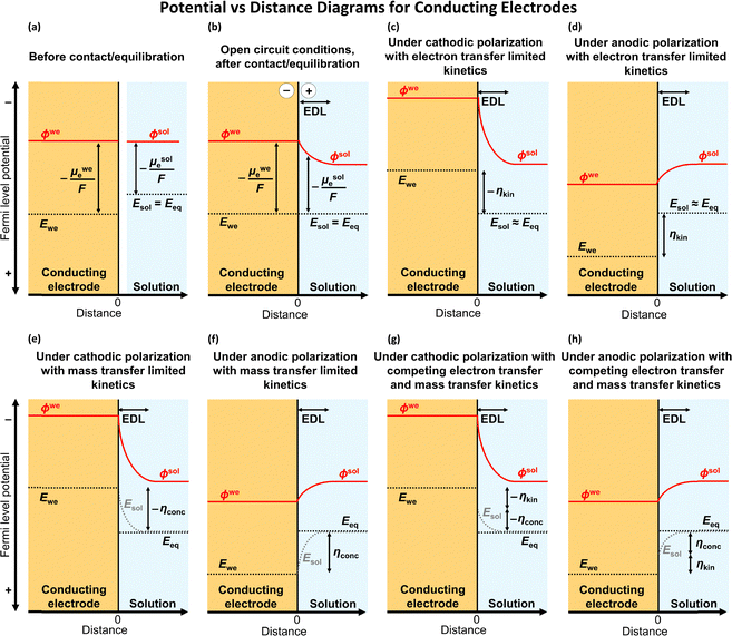 |
| | Fig. 2 Potential versus distance diagrams depicting electrochemical equilibration across the interfaces of conducting working electrodes and solution phases. (a) Before contact of the electrode and solution phases, the solution potential (Esol) is equilibrated with the bulk equilibrium potential (Eeq) but differs in value from the Fermi-level potential of the working electrode (Ewe). μwee and μsole are chemical potentials of electrons in the working electrode and the solution phase, respectively, and ϕwe and ϕsol are the electric potentials in the working electrode and in the solution phase, respectively. (b) Upon contact of the electrode and solution phases, interfacial electron transfer results in an accumulation of negative charges on the electrode surface and positive charges in the solution, creating a gradient of the electric potential (ϕα) that appears predominantly across the solution phase and within the electric double layer (EDL). At equilibrium, the Fermi levels across the phases are flat, meaning Ewe, Esol, and Eeq are spatially and temporally equal in value. (c) and (d) When the interfacial electron-transfer kinetics are relatively sluggish compared with mass-transfer kinetics [and thus the solution potential at the electrode surface (Esol)s is approximately equal to Eeq], cathodic (panel c) or anodic (panel d) polarization of the working electrode increases the electric potential gradient across the EDL, resulting in an overpotential (η) that is dominated by the kinetic overpotential (ηkin). In this figure, the solution potential at the electrode surface (Esol)s is the value of Esol at distance = 0 on the x-axis. (e) and (f) When the kinetics of interfacial electron transfer are relatively fast compared with the kinetics of mass transfer [and thus the value of (Esol)s is equal to the value of Ewe], cathodic (panel e) or anodic (panel f) polarization of the working electrode results in an increase in the electric potential gradient across the EDL and η, which is dominated by the concentration overpotential (ηconc). (g) and (h) When the kinetics of interfacial electron transfer competes with the kinetics of mass transfer [and thus the value of (Esol)s can be different from Eeq and Ewe, cathodic (panel g) or anodic (panel h) polarization of the working electrode results in an increase in the electric potential gradient across the EDL and η that is the sum of ηkin and ηconc. | |
Because conducting/metallic electrodes have a relatively high density of electronic states at the Fermi level (compared with those in molecules and semiconductors), the electron concentrations in conducting electrodes are relatively high (∼1022 cm−3) compared with those in solution phases, where electrons are localized on reduced and oxidized forms of chemical species (∼1018–1019 cm−3 for solutions that are 10–100 mM in chemical species).6,8 By extension, conducting working electrodes have relatively high capacitance (C, with units of C V−1 and defined as the ratio of the change in electric charge to the corresponding change in electric potential)8 per unit area compared with that of electrolyte solutions. Thus, any resulting drop in electric potential upon biasing a conducting working electrode in contact with a solution phase appears predominantly in the solution phase and across the EDL. We note that the SI (International System of Units) unit for capacitance is the Farad (often expressed as F and not to be confused with the Faraday constant, which is commonly expressed as F).
Leveraging the concepts and terms defined thus far, we are positioned to introduce the term overpotential (η, with units of V and defined as the Gibbs free energy per charge of one mole of electrons used to drive an electrochemical reaction away from equilibrium, and thus equal to the difference between the applied electrode potential, Eapp, and the equilibrium potential, Eeq), as expressed in eqn (19),5,33
| | | η = Eapp − Eeq (the overpotential). | (19) |
In accordance with
eqn (19),
Eapp supplied to a conducting electrode requires sufficient thermodynamic poise with respect to
Eeq to drive an electrochemical reaction in the forward direction (meaning an overall negative change in Gibbs free energy is required for spontaneity). This definition of the overpotential will be used later to define what has been referred to in the literature as an “underpotential,”
36–39 where
Eapp is polarized at potentials that are thermodynamically insufficient to drive the reaction with respect to
Eeq. Nonetheless, as further detailed later in this review article, semiconducting electrodes can drive reactions even when
Eapp is insufficient in thermodynamic poise with respect to
Eeq.
This is not a violation of thermodynamics and occurs because photons bring additional energy that can supply a “photovoltage” (see Section IV on overpotentials and underpotentials in semiconductor photoelectrochemistry). In the following Section F, we review the connection between overpotentials and currents.
F. How overpotentials influence electron transfer kinetics and the flow of currents in conducting electrodes
Consider a relatively simple one-electron transfer reaction (i.e., Ox + e− ⇄ Red and the converse Red ⇄ Ox + e−) at the interface of a working electrode phase and a solution phase. When the Fermi-level potential of the working electrode, Ewe, is polarized at an applied electrode potential, Eapp, [see Fig. 2(c)–(h)], the anodic heterogeneous electron transfer rate constant (kETa, with units of m s−1, yet commonly reported with units of cm s−1, and defined as the proportionality constant relating the rate of the interfacial electron transfer reaction to the concentration of Red at the electrode|solution interface)40 and the cathodic heterogeneous electron transfer rate constant (kETc, with units of m s−1, yet commonly reported with units of cm s−1, and defined as the proportionality constant relating the rate of the interfacial electron transfer reaction to the concentration of Ox at the electrode|electrolyte solution interface)40 are expressed using eqn (20a) and (20b),| |  | (20a) |
| |  | (20b) |
where β is the symmetry factor (which is a dimensionless coefficient quantifying the symmetry of the energy barrier between reactant and product states of electrode reactions involving a single one-electron transfer step),5,41,42 and  is the standard heterogeneous electron transfer rate constant (with units of m s−1, yet commonly reported with units of cm s−1, and defined as the value of heterogeneous electron transfer rate constants of the anodic and cathodic reactions under standard conditions).5,40 Thus, under standard conditions, and when the working electrode potential, Ewe, is equilibrated with the equilibrium potential, Eeq, of the solution phase [see Fig. 2(b)], the values of kETa, kETc, and
  are equivalent. Further, for electron transfer reactions involving conducting electrodes, the concentration of electrons in the electrode phase is effectively constant and independent of the applied electrode potential. Changes in overpotential do, however, alter the activation energy (due to the electric potential dropping across the EDL) and hence the rate constants for electron transfer.43
When an applied bias potential, Eapp, is used to poise Ewe away from Eeq and introduce an overpotential, if the kinetics of interfacial electron transfer are relatively sluggish compared with mass transport to or from the electrode and from or to the bulk electrolyte solution, then the concentrations of chemical substrates at the electrode surface will remain approximately equal to their bulk values,  and
and  . Correspondingly, the solution potential at the electrode surface, (Esol)s, will be approximately equal to the equilibrium potential [i.e., across the solution phase Esol ≈ Eeq and thus (Esol)s ≈ Eeq, as illustrated in Fig. 2(c) and (d)]. Under such conditions, the current density (J, with units of A cm−2 and defined as the amount of charge flowing through a cross-section perpendicular to the flow per unit cross-sectional area and unit time)8 can be described using the form of the Butler–Volmer equation shown in eqn (21),
| |  | (21) |
where
J0 is the
exchange current density (with units of A cm
−2 and defined as the absolute value of the equal-magnitude anodic and cathodic currents that comprise the dynamic equilibrium when
Ewe =
Eeq), as expressed in
eqn (22),
| | 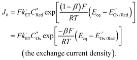 | (22) |
The values of
J0, are thus relatively low when net currents are limited by rates of heterogeneous electron transfer, and not the transport of chemical substrates (corresponding to

values ∼< 3.0 × 10
−5 cm s
−1). Under these conditions the reaction is termed
electrochemically irreversible and any applied overpotential,
η, is dominated by
kinetic overpotential [
ηkin, with units of V and defined as the difference between
Eapp and (
Esol)
s as expressed by
eqn (23), which is the component of the overpotential required to overcome the activation energy for heterogeneous electron transfer] [see
Fig. 2(c) and (d)],
| | | ηkin = Eapp − (Esol)s (the kinetic overpotential). | (23) |
If the kinetics of interfacial electron transfer are relatively fast compared with the transport of chemical substrates, Nernstian equilibrium is maintained at the electrode|electrolyte solution interface when
Ewe is poised away from
Eeq [meaning
Ewe = (
Esol)
s, as illustrated in
Fig. 2(e) and (f)]. Under these conditions, the concentrations of chemical substrates at the interface deviate from those in the bulk solution.
31,44 Under these conditions, the reaction is termed
electrochemically reversible, and the values of
J0 are relatively large (corresponding to

values ∼> 0.020 cm s
−1). Further, any applied
η will be dominated by
concentration overpotential [
ηconc, with units of V and defined as the difference between (
Esol)
s and
Eeq as expressed by
eqn (24), which is the component of the overpotential associated with changing the surface concentrations of chemical substrates] [see
Fig. 2(e) and (f)],
| | | ηconc = (Esol)s − Eeq (the concentration overpotential). | (24) |
When the value of the exchange current density,
J0, is intermediate (corresponding to values of
k°ET ranging from

), the reaction is termed
electrochemically quasi-reversible. Since
J0 is larger than that of an electrochemically irreversible reaction, both anodic and cathodic processes contribute to the net current.
5 At relatively lower overpotentials, the net currents will be predominantly limited by heterogeneous electron transfer. Conversely, at relatively higher overpotentials, the net currents will be predominantly limited by mass transport. Thus, under electrochemically quasi-reversible conditions, the applied
η is the sum of
ηkin and
ηconc, as indicated in
eqn (25) [see
Fig. 2(g) and (h)],
| | | η = ηkin + ηconc (the overpotential expressed as a sum of kinetic and concentration components). | (25) |
All kinetic theories require the kinetic equations to collapse to thermodynamic relations at equilibrium. In the case of the Butler–Volmer equation, it reduces to the Nernst equation when equilibrium conditions are applied. Conversely, at relatively high polarization conditions, the Butler–Volmer equation explains Tafel behavior and reduces to the empirical
Tafel equation,
45 which relates the rate of an electrochemical reaction to the overpotential. The range of

values relating to definitions of electrochemical reversibility is summarized in
Table 1. Although not detailed in this article, there are extended forms of the Butler–Volmer equation that account for mass transport limitations and describe the diffusion-limited region of current–overpotential curves.
5 Further details on the Tafel equations, including their applications in the benchmarking of catalysts are covered in the subsequent Section III on overpotentials in electrocatalysis.
Table 1 Range of the heterogeneous electron transfer rate constant and electrochemical reversibility
III. Overpotentials in electrocatalysis (heterogeneous and homogeneous)
A. Overview of electrocatalysis and heterogeneous versus homogeneous conditions
Electrocatalysis is defined as the process of utilizing catalysts to accelerate electrochemical reactions.46,47 Electrocatalysts provide alternative, lower-energy pathways for driving electrochemical transformations. Electrocatalysts are therefore central to biological and technological energy-conversion processes because they differentiate between competing reaction rates and thereby improve the selectivity and overall efficiencies for producing a desired chemical product.48
Classifications of electrocatalysis include heterogeneous electrocatalysis (where the catalysts and chemical substrates reside in distinct phases) and homogeneous electrocatalysis (where the catalysts are in the same phase as the chemical substrates).46 However, work on clusters, metal nanoparticles, nanomaterials, and molecular species interfaced with solid supports has blurred the boundaries between heterogeneous and homogeneous catalysis.49 Such distinctions are further complicated by the emergence of hybrid constructs featuring molecular active sites that exhibit strong electronic coupling with the band states of the solid material.50–52 To facilitate comparisons of underlying mechanisms associated with heterogeneous versus homogeneous catalysts, in subsequent Sections B and C we initially review heterogeneous electrocatalysis where solid materials with non-uniform surface structures and a continuum of electronic states catalyze the reactions. These heterogeneous reactions proceed via mechanisms involving inner-sphere electron transfer, defined as reactions where the electron transfer occurs with a relatively strong electronic coupling (∼>20 kJ mol−1) between the electron donor and acceptor.8 In subsequent Sections D and E, we then review homogeneous electrocatalysis, where molecular species with well-defined three-dimensional and electronic structures catalyze the reactions. These homogeneous reactions proceed via mechanisms involving outer-sphere electron transfer, defined as reactions where the electron transfer occurs with no or relatively weak electronic couplings (∼<20 kJ mol−1) between the electron donor and acceptor.8 As indicated in Fig. 3, in addition to their heterogeneous versus homogeneous nature, electrocatalytic reactions can also be distinguished as involving chemical catalysis (which involves bonded interactions between the active form of the catalyst and the substrate to enable increases in catalytic efficiency and specificity, including stereospecificity) and/or redox catalysis (which refers to catalysts acting as an outer-sphere electron transfer agent, with electrons being transferred and dispersed in three-dimensional space).53
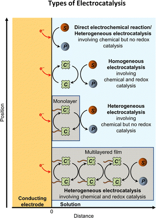 |
| | Fig. 3 Schematic representation of the various types of catalysis, including direct electrochemical reaction/heterogeneous catalysis, homogeneous catalysis, immobilized monolayer chemical but no redox catalysis, and multilayer chemical and redox catalysis of electrochemical reactions. Shaded areas represent a monolayer or multilayer film of catalysts. Molecular catalysts immobilized as monolayer or multilayered coatings deposited on electrode surfaces are considered examples of heterogeneous catalysis, even though they involve molecular components, because the catalysts and chemical substrates are in distinct phases and catalysis takes place at the electrode interface. Adapted with permission from Savéant, J.-M., 2008. Copyright 2008 American Chemical Society. | |
B. Overpotentials in heterogeneous electrocatalysis
General steps of a heterogeneous electrocatalytic reaction are depicted in Fig. 4(a). In this example, a chemical substrate (S) traverses the electric double layer, EDL, and forms a bond with a catalytic metal site on an electrode surface, generating an adsorbed species. Because the catalytic metal site that binds with the chemical substrate is strongly coupled to the delocalized band states in the electrode and any external circuitry, this bond-forming step occurs inherently via concerted electron transfer.54
 |
| | Fig. 4 (a) A mechanistic scheme involving interfacial inner-sphere electron transfer resulting in bond formation between an electrode surface site and a chemical substrate (S). (b) A Fermi-level potential versus distance diagram depicting a heterogeneous electrocatalyst|electrolyte solution interface, where catalysis proceeds through an inner-sphere electron transfer mechanism. In this diagram, Eapp represents the applied electrode potential, Ecat is the catalyst potential, Eeq is the equilibrium potential, ϕsol is the electric potential in the solution phase, and ϕwe is the electric potential in the working electrode phase. In this example, negative polarization of the working electrode would raise both Eapp and Ecat, and increase the magnitude of the overpotential (η). (c) A Gibbs free energy diagram illustrating an electrocatalytic reduction proceeding via a mechanism involving inner-sphere electron transfer, where a catalytic electrode surface site (M) reacts with S to form a catalyst–substrate reaction intermediate (M–S). In this diagram, Eapp and  represent applied electrode potentials, ΔḠ‡s and represent applied electrode potentials, ΔḠ‡s and  represent changes in standard Gibbs free energy of activation for forming a catalyst–substrate reaction intermediate, and represent changes in standard Gibbs free energy of activation for forming a catalyst–substrate reaction intermediate, and  and and  represent changes in standard Gibbs free energy for forming a catalyst–substrate reaction intermediate at the respective applied electrode potentials of Eapp or represent changes in standard Gibbs free energy for forming a catalyst–substrate reaction intermediate at the respective applied electrode potentials of Eapp or  . Individual electron transfer or intermediate steps are not depicted for simplicity. (d) A mechanistic scheme involving interfacial outer-sphere electron transfer between an electrode and a homogeneous molecular catalyst (C). (e) A Fermi-level potential versus distance diagram depicting a conducting electrode|homogeneous catalyst solution interface, where catalysis proceeds through outer-sphere electron transfer. A negative polarization of the working electrode increases the driving force for outer-sphere electron transfer from the electrode to the catalyst, whereas the driving force for substrate activation (ηeff) is determined by the standard reduction potential of the catalyst . Individual electron transfer or intermediate steps are not depicted for simplicity. (d) A mechanistic scheme involving interfacial outer-sphere electron transfer between an electrode and a homogeneous molecular catalyst (C). (e) A Fermi-level potential versus distance diagram depicting a conducting electrode|homogeneous catalyst solution interface, where catalysis proceeds through outer-sphere electron transfer. A negative polarization of the working electrode increases the driving force for outer-sphere electron transfer from the electrode to the catalyst, whereas the driving force for substrate activation (ηeff) is determined by the standard reduction potential of the catalyst  and is independent of the applied potential. (f) A Gibbs free energy diagram illustrating an electrocatalytic reduction proceeding via an outer-sphere electron transfer mechanism, where C is activated via electron transfer to form an activated form of the catalyst (C′), which further reacts with a S to form a catalyst–substrate reaction intermediate (C–S). ΔḠ‡ET and and is independent of the applied potential. (f) A Gibbs free energy diagram illustrating an electrocatalytic reduction proceeding via an outer-sphere electron transfer mechanism, where C is activated via electron transfer to form an activated form of the catalyst (C′), which further reacts with a S to form a catalyst–substrate reaction intermediate (C–S). ΔḠ‡ET and  are changes in standard Gibbs free energy of activation for interfacial electron transfer from the electrode to the catalyst at applied electrode potentials of Eapp or are changes in standard Gibbs free energy of activation for interfacial electron transfer from the electrode to the catalyst at applied electrode potentials of Eapp or  , respectively, and , respectively, and  and and  are the changes in standard Gibbs free energy for interfacial electron transfer from the electrode to the catalyst at applied electrode potentials of Eapp or are the changes in standard Gibbs free energy for interfacial electron transfer from the electrode to the catalyst at applied electrode potentials of Eapp or  . Only the highest-energy barriers for the electron transfer and substrate activation are depicted for simplicity. Although the figures illustrate cathodic reactions, related concepts apply to anodic reactions, where positive polarization of the working electrode increases the driving force for activating chemical substrates in the bulk solution (via inner-sphere mechanisms) or the driving force for activating the homogeneous catalysts (via outer-sphere mechanisms) to increase the rate of oxidation reactions. . Only the highest-energy barriers for the electron transfer and substrate activation are depicted for simplicity. Although the figures illustrate cathodic reactions, related concepts apply to anodic reactions, where positive polarization of the working electrode increases the driving force for activating chemical substrates in the bulk solution (via inner-sphere mechanisms) or the driving force for activating the homogeneous catalysts (via outer-sphere mechanisms) to increase the rate of oxidation reactions. | |
The catalyst potential (Ecat, with units of V vs. Eref and defined as the Fermi-level potential of the catalyst) can be expressed in terms of the electrochemical potential of the electrons in the catalyst phase (cate), or in terms of the catalyst standard potential  , as shown in eqn (26),
| |  | (26) |
where
acatcatOx and
acatcatRed are activities of Ox and Red forms of catalytic sites, respectively, in the catalyst phase. Because the catalytic metal sites of heterogeneous catalysts are part of the electrode and reside within the EDL,
Ecat is considered to be in electrostatic equilibrium with the applied electrode potential,
Eapp. This means that the orbital energy levels of the catalytic metal site, described by the term
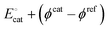
in
eqn (26), shift in response to changes in the bias potential.
50–52,55,56 When the heterogeneous catalytic sites are part of—and thus integral to—a working electrode, the Fermi-level potentials of the working electrode,
Ewe, and the catalysts,
Ecat, will track with each other when biasing the working electrode. Thus, polarizing the working electrode with respect to a reference electrode will not provide additional driving force for electron transfer between the working electrode and the catalysts [see
Fig. 4(b) depicting an example involving a cathodic reaction]. Polarizing the working electrode does however alter the magnitude of the electric potential drop across the EDL.
50,52,55–57
The tracking of Ecat with Eapp (and thus Ewe) during heterogeneous electrocatalysis is also captured in the Gibbs free energy diagram depicted in Fig. 4(c). In this diagram depicting the free energy profile along a reaction pathway, the reaction coordinate is the collection of motions of atoms, including changes in the distances between atoms and the degrees of bond angles that are directly involved in the formation of products from reactants.8,12 The configuration of atoms corresponding to the highest Gibbs free energy is the transition state of the reaction, whereas the clusters of atoms corresponding to positions near the maximum Gibbs free energy are more loosely referred to as activated complexes.8,12 For the diagram illustrated in Fig. 4(c), the progression along the reaction yields a reaction intermediate (i.e., a chemical species that exists during a chemical reaction with a lifetime appreciably longer than a molecular vibration and reacts further to give the products)8 abbreviated as M–S to indicate a catalyst bound to its substrate. In this example, involving a cathodic reaction, setting the value of Eapp negative of the equilibrium potential, Eeq, (and by extension setting the value of Ecat negative of Eeq) provides a driving force for reducing the chemical substrate and establishes the overpotential, η. Thus, negatively shifting Eapp to  , as indicated in Fig. 4(c), increases the magnitude of the standard Gibbs free energy change for forming the catalyst–substrate reaction intermediate [indicated as
  and
and  in Fig. 4(c), with units of J mol−1 and defined as the Gibbs free energy change associated with formation of the catalyst–substrate reaction intermediate].50 Consistent with the Butler–Volmer equation and Marcus–Hush–Levich theory,41,44,58 in addition to setting the thermodynamic driving force for the electron-transfer reaction, the overpotential also influences the electrochemical reaction kinetics by modulating the potential-dependent change in standard Gibbs free energy of activation for forming a catalyst–substrate reaction intermediate [indicated as ΔḠ‡s and
  in Fig. 4(c), with units of J mol−1 and defined as the Gibbs free energy required to form the transition state structure]. Nonetheless, the overpotential is a thermodynamic parameter.
C. Benchmarking of heterogeneous electrocatalysts
The benchmarking of heterogeneous electrocatalysts has been pursued using thermodynamic and kinetic parameters obtained from the analysis of Tafel plots [Fig. 5(a)], which relate the overpotential, η, to the log of the absolute value of electrocatalytic current density, log |j|. Mathematically, Tafel plots for one-electron transfer reactions are described by Tafel equations [eqn (27a) and (27b)],| |  | (27a) |
| |  | (27b) |
where the exchange current density, J0, is obtained by extrapolating the linear segments of a Tafel plot to zero overpotential. Since a heterogeneous catalyst that exhibits a larger J0 will require a smaller overpotential to achieve a desired current density, J0 provides a benchmarking parameter that gives a measure of the catalyst's ability to deliver a net current without a significant energy loss due to activation.5 Plotting experimentally measured J0 values versus some metric of adsorption or binding strength between the catalyst and its substrate yields a “volcano-type” plot [see Fig. 5(b)]. These types of plots are attributed to first being introduced by Balandin59 and provide a quantitative illustration of the Sabatier principle,60 which states that efficient catalysis occurs when the catalyst binds its reactant with an intermediate strength because structural features that favor tight binding of reactants also tend to inhibit the release of products.61 Thus, the maximum rate of catalysis occurs when the binding is “just right” and at the apex of the “volcano.”62,63
 |
| | Fig. 5 (a) Tafel plots showing the anodic and cathodic branches of current-overpotential curves of a one-electron transfer reaction. (b) A volcano-type plot illustrating the Sabatier principle. In this plot, fast catalysts appear near the apex of the “volcano” where the reaction rate is maximized, and the binding is “just right”. | |
In addition to the exchange current density, the Tafel slope provides another benchmarking parameter and offers insights regarding catalytic reaction mechanisms.64 For an electrode reaction involving a single electron-transfer step, the slopes of the anodic and cathodic segments of the Tafel plot are (1 − β)F/2.3RT and −βF/2.3RT, respectively. For generic electrode processes involving transfer of more than one electron and/or chemical steps, the slope is expressed by eqn (28a) and (28b),65
| |  | (28a) |
| |  | (28b) |
where
αa is the
anodic transfer coefficient (which is a dimensionless coefficient quantifying the fraction of applied potential that influences the rate of an anodic reaction), and
αc is the
cathodic transfer coefficient (which is a dimensionless coefficient quantifying the fraction of applied potential that influences the rate of a cathodic reaction).
42 The transfer coefficients and, by extension, the Tafel slopes can be estimated using the quasi-equilibrium method, which assumes all the reaction steps are in equilibrium except for the rate-determining or rate-limiting step (
i.e., an elementary step that is much more sluggish than all the others and thus sets the overall reaction rate).
65,66 The experimentally observed Tafel slopes can then be compared with theoretically derived slopes to elucidate reaction mechanisms. For example,
αc is equal to
β, and
αa to (1 −
β) for a simple one-electron transfer reaction. Specifically, if the first electron transfer for an anodic reaction is rate-limiting and the potential energy barrier is symmetric (
i.e.,
β = 0.5), the value of the Tafel slope should be 4.6
RT/
F, which is equivalent to 118 mV dec
−1 at 298 K. Nonetheless, caution is advised in applying the terms
β, 1 −
β,
αc, and
αa. Unlike the terms
β and 1 −
β, which are specific to transformations at an electrode involving a single one-electron transfer step and are thus only relevant to the physical chemistry of an elementary electron transfer step, the terms
αc and
αa encompass additional mechanistic factors relevant to overall multi-electron-step and/or multi-chemical-step electrode reactions. These factors include the number of electrons transferred before the rate-determining or rate-limiting step and the number of times the rate-determining or rate-limiting step must be engaged to complete one occurrence of the overall reaction.
42 Further complications can arise when suppositions are applied to simplify analyses. For example, kinetic models can fail when assumptions, including that the surface coverage of intermediate species is independent of the applied electrode potential, are inappropriate for describing the surface electrocatalysis and microkinetic models.
64
In general, caution should be exercised when benchmarking heterogeneous catalysts because the dominant contribution to catalytic activity may come from hard-to-identify minority sites, such as defects.67 Reporting catalytic currents using standardized approaches could enable more meaningful comparisons of different catalyst materials, but converging on such standards (and any related specific experimental conditions, including pH) will be challenging. It is also informative to consider whether catalytic current densities are reported with respect to the electrochemically active surface area (ECSA) (i.e., the electrochemically active area of an electrode that is accessible to the electrolyte) or a geometric surface area (i.e., the interfacial area of an electrode determined on the assumption that the interface is flat).68 However, a universal method to determine the ECSA of materials in more complex electrochemical environments remains challenging and limits abilities to benchmark the performance of heterogeneous catalysts.67
D. Overpotentials in homogeneous/molecular electrocatalysis
General steps of a homogeneous electrocatalytic reaction are depicted in Fig. 4(d). In this example, electrons—rather than chemical substrates—traverse the EDL to reduce a molecular catalyst (C) and generate an activated form of the catalyst (C′). Following activation of the catalyst, C′ reacts with the chemical substrate (S) to yield the product (P) while regenerating C. Since homogeneous catalysts have their own unique electronic properties that are separate from the electrode's, the standard reduction potential of the catalyst [ , with units of V vs. Eref and representative of the electrode potential where half of the total number of catalysts (C + C′) at the interface of the electrode and catalyst-containing electrolyte solution are present in their activated form, C′] does not track with the applied electrode potential, Eapp, and instead remains constant in value. As indicated in eqn (29), the difference between the equilibrium potential, Eeq, and
  sets the value of the effective overpotential (ηeff, with units of V),
| |  | (29) |
For the potential versus distance diagram shown in Fig. 4(e), polarizing the working electrodes alters the overpotential [which remains defined as the difference between Eapp and Eeq as expressed in eqn (19)]; however, the effective overpotential remains unchanged. Nonetheless, polarizing the working electrode does alter the magnitude of the electric potential drop across the EDL, and increases the difference between the applied electrode potential, Eapp, and the catalyst standard potential,  , providing further driving force8,69 for activating the catalyst.
The distinctions between overpotential and effective overpotential during homogeneous electrocatalysis are also captured in the reaction coordinate diagram depicted in Fig. 4(f). In this example involving a cathodic reaction, negatively shifting the value of Eapp to  , as indicated in Fig. 4(f), increases the magnitude of the potential-dependent standard Gibbs free energy change for electron transfer from the electrode to the catalyst [
 or
or  in Fig. 4(f), with units of J mol−1 and defined as the difference in standard Gibbs free energy between the reactant state (i.e., prior to interfacial electron transfer) and the product state (i.e., following interfacial electron transfer)].50,52,55 In general, a cathodic biasing of Eapp for a reductive electrochemical transformation also lowers the change in standard Gibbs free energy of activation for electron transfer from the electrode to the catalyst [indicated as
  and
and  in Fig. 4(f), with units of J mol−1 and defined as the difference in standard Gibbs free energy between the reactant state and transition state structures associated with the electron transfer]. However, as opposed to heterogeneous catalysis, polarizing the working electrode does not alter the thermodynamics of chemical steps associated with catalyst–substrate binding when the electron transfer and catalyst–substrate binding proceed via stepwise mechanisms rather than concerted pathways. The standard Gibbs free energy change for forming a catalyst–substrate reaction intermediate,
  , consequently, does not change when modulating Eapp. By extension, changing the value of Eapp does not influence the standard Gibbs free energy of activation for forming a catalyst–substrate reaction intermediate,
  in Fig. 4(f). Thus, under an appropriate bias, the maximum reaction rate can become independent of Eapp and limited by kinetics associated with chemical catalysis.57
E. Benchmarking of homogeneous electrocatalysts
The benchmarking of homogeneous electrocatalysts is achieved by comparing intrinsic catalytic properties that are independent of the characteristics of an electrochemical cell.70 One kinetic performance metric of a catalyst is the turnover frequency (TOF, with units of s−1). As shown in eqn (30), TOF is defined as the ratio of the moles of product generated over a specified unit of time during which the catalyst is stable (Nproduct, with units of mol s−1) versus the total amount of catalyst contained within the reaction-diffusion layer, (Ncat, with units of mol), where the reaction-diffusion layer is the region proximal to the electrode surface where the concentration profiles of electro-activated versus nonactivated catalysts vary from their bulk values,| | 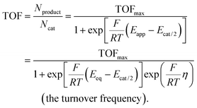 | (30) |
In the absence of electron- and mass-transfer limitations, and if the electrode activity were limited only by kinetics relevant to chemical catalysis, all catalysts at the electrode surface would be present in their activated form, and the concentration of chemical substrates at the electrode surface would be approximately equal to their bulk values. Under such conditions, the voltammograms will display an “S-shaped” waveform [see Fig. 6(a)], and the magnitude of the current recorded in the plateau region of the voltammogram trace will be independent of the scan rate.
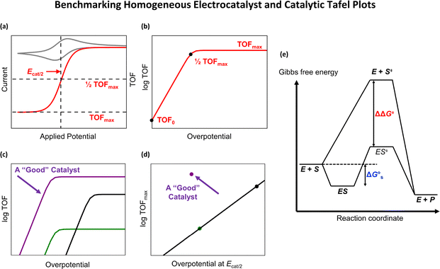 |
| | Fig. 6 (a) Voltammograms associated with either the interconversion between oxidized and reduced forms of an electroactive species in solution (i.e., a duck-shaped voltammogram) (gray), or a catalytic reaction involving an irreversible catalytic step where the concentration of the chemical substrate is sufficiently high to maintain a concentration at the electrode surface that is essentially the same as the bulk concentration (red). The maximum turnover frequency (TOFmax), half the maximum turnover frequency (1/2 TOFmax), and the half-wave potential of the steady-state catalytic wave (Ecat/2) are indicated with dashed lines. (b) A catalytic Tafel plot constructed for a molecular electrocatalyst showing TOFmax, 1/2 TOFmax, and the intrinsic turnover frequency (TOF0). At sufficient overpotential, the turnover frequency (TOF) approaches an asymptotic value of TOFmax. (c) Catalytic Tafel plots and (d) a plot correlating TOFmax and Ecat/2. In these plots, a “good catalyst” features a relatively high TOFmax as well as a low effective overpotential (i.e., the overpotential at Ecat/2) and is thus positioned in the upper left of the Cartesian coordinate indicated in panels c and d of this figure. (e) Reaction coordinate diagrams comparing an uncatalyzed reaction, passing through the transition state labeled E + S‡, and an enzyme-catalyzed reaction, passing through a lower energy transition state labeled ES‡. In this figure, the relative stabilization of the enzyme-catalyzed transition state (ΔΔG‡) is greater than the standard Gibbs free energy change for activating the substrate  to form an enzyme-substrate complex, indicating the relatively high specificity of enzymes for binding an “activated complex.” Panels a and b were adapted with permission from Nishiori et al., 2021. Copyright 2021 Chemical Catalysis. to form an enzyme-substrate complex, indicating the relatively high specificity of enzymes for binding an “activated complex.” Panels a and b were adapted with permission from Nishiori et al., 2021. Copyright 2021 Chemical Catalysis. | |
As further indicated in eqn (30), TOF can be expressed as a function of the overpotential, η, and the maximum turnover frequency (TOFmax, with units of s−1 and defined as the highest per-active-site rate at which a catalyst can convert reactant molecules into product molecules). Unlike TOF—which is a function of the applied electrode potential—TOFmax is a potential-independent rate constant that provides a kinetic benchmarking parameter. The value of TOFmax also establishes a related thermodynamic benchmarking parameter termed the half-wave potential of the steady-state catalytic wave (Ecat/2, with units of V vs. Eref), which is the applied electrode potential required to activate half the catalysts at the electrode surface, and thus the potential required for a molecular electrocatalyst to operate at half the value of TOFmax.71,72
The logarithmic plot of the turnover frequency, TOF, of a molecular catalyst versus overpotential, η, shown in Fig. 6(b) is called a catalytic Tafel plot. Such plots facilitate benchmarking of molecular catalysts and the extraction of intrinsic catalytic properties, including TOFmax (as indicated by the asymptotic value of TOF), Ecat/2, (as indicated by the ‘elbow’ of the plot and the overpotential at 1/2 TOFmax), and the intrinsic turnover frequency (TOF0, with units of s−1 and defined as an extrapolated TOF at zero overpotential). The relationship between TOF0 and TOFmax is expressed in eqn (31),
| |  | (31) |
TOF
0 is somewhat analogous to the exchange current density,
J0, given both terms represent rates under equilibrium conditions, and are intrinsic catalytic properties.
73 To extend the concepts of exchange current density and electrochemical reversibility to electrocatalysis involving molecules attached to electrodes (
i.e., heterogenized molecular catalysts), Armstrong and Hirst adopt the term “electrocatalytic exchange current.”
31 This term encompasses kinetics associated with interfacial electron transfer, turnover of the catalytic center, and any intramolecular electron-transfer steps—each of which may limit the overall rate of electrocatalysis. Like the exchange current density, the electrocatalytic exchange current is defined at the equilibrium potential,
Eeq, and not at the potential of any redox centers associated with the electrocatalyst. Molecular electrocatalysts with relatively high electrocatalytic exchange currents and low overpotential requirements are deemed reversible and efficient. Conversely, electrocatalysts with relatively low electrocatalytic exchange currents and high overpotential requirements are considered irreversible and inefficient.
31
Catalytic Tafel plots constructed for molecular catalysts show that using electron-withdrawing or electron-donating groups to improve overpotential requirements (thermodynamics) adversely affects reaction kinetics and the maximum turnover frequency a complex achieves [as depicted in Fig. 6(c) and (d)].74 One rationalization for this observation is that structural features favoring electron transfer at lower overpotentials tend to adversely affect kinetics associated with chemical steps involving the binding/unbinding of protons or other nucleophilic steps. In other words, scaling-type relationships exist75 due to the trade-offs between electrophilicity and nucleophilicity. This molecular scaling relationship has some conceptual parallels with the volcano-type plots associated with catalytic transformations occurring at heterogeneous metallic surfaces and with the Sabatier principle.60–63 When protons are a chemical substrate, as they are for nearly all fuel-forming reactions relevant to solar photochemistry, the binding affinities of substrate protons are quantified as pKas or pKbs. In a somewhat related vein, but with salient distinctions, to the classic works of Sabatier and Balandin indicating a good catalyst is “just right” in terms of binding reactants and products, Pauling emphasized how good catalysts—including enzymatic proteins—provide appropriate three-dimensional environments for tightly binding a transition state [see Fig. 6(e)].76,77 Nonetheless, in the context of multi-electron, multi-chemical-step processes, the use of a single descriptor to account for these more complicated processes is perhaps an oversimplified approach.74
In summary, applications of voltammetry have revealed previously unexplored dimensions of thermodynamic and kinetic parameters and enable the benchmarking of molecular electrocatalysts via determining their maximum turnover frequency, TOFmax, and effective overpotential, ηeff, values. The concept of turnover frequency, TOF, has been applied to applications involving heterogenized molecular catalysts. However, in these cases, the definition of TOF is less precise, and caution is advised to determine how the authors define and use this term. For example, the TOF could be based on the activity per total loading of catalyst or the electroactive loading of catalysts. Given the inherent structural diversity of catalytic sites in heterogeneous assemblies, the TOF in these cases is perhaps better viewed as an “average TOF,” as opposed to a well-defined parameter of a homogeneous molecular species. In addition to limitations associated with potential-dependent electron transfer kinetics in the case of electrocatalysis, the situation can become further complicated in cases involving photoelectrochemical reactions, where the flux of photons can limit the photoelectrosynthetic activities (vide infra).78
IV. Overpotentials and underpotentials in semiconductor photoelectrochemistry
A. Overview of semiconductor photoelectrochemistry
Semiconductor photoelectrochemistry involves the application of light-absorbing semiconductors as photoelectrodes in contact with an electrolyte solution.79–82 In such assemblies, charge carriers (i.e., particles that move within a material and carry an electric charge, enabling the flow of current) generated via photon absorption by the electrodes can drive redox transformations in the solution phase.83,84 These assemblies are thus excitonic chemical conversion systems, which utilize light to promote chemical reactions.85 The interchangeable use of “photocatalytic” and “photosynthetic” is therefore discouraged, as the overall thermodynamics of the related reactions distinguishes these terms.85Photocatalytic reactions are exergonic (i.e., the Gibbs free energy change is negative, ΔG < 0, meaning there is no net chemical energy storage, but light accelerates the reaction kinetics). Conversely, photosynthetic reactions are endergonic (i.e., the Gibbs free energy change is positive, ΔG > 0, meaning photonic energy is stored in the form of chemical bonds).79,85 In Sections B–E, we review the thermodynamic and kinetic principles relevant to photoelectrosynthetic assemblies featuring semiconductor photoelectrodes that utilize the energy of photons to drive thermodynamically uphill reactions.
B. Band-edge potentials and Fermi levels in semiconductors
The electronic structures of solid-state materials are described via the “band model”.86,87 When isolated atoms are assembled in a lattice to form a crystalline solid, overlap of the atomic orbitals creates new molecular orbitals, which are closely spaced in energy and merge to form continuous electronic states called bands.8 The highest-energy continuum of electronic states, consisting of the bonding orbitals that are fully occupied by electrons at the absolute zero temperature, is the valence band. The lowest-energy continuum of electronic states, consisting of the antibonding orbitals that are vacant at the absolute zero temperature, is the conduction band.15 In semiconductors, the valence and conduction bands are separated in energy by a “forbidden” region where no states exist, called the band gap. The difference in energy between the lowest-energy electronic state of the conduction band and the highest-energy electronic state of the valence band is the band gap energy (εg, with units of eV).8 When the band gap of a material is relatively large (i.e., εg is larger than approximately 4 eV), and under conditions where the valence band of the material is occupied by electrons and the conduction band is unoccupied,88 the material will exhibit relatively little to no electrical conductivity and is classified as an insulator. In contrast, when the band gap of a material is relatively small (i.e., εg ≪ kT = 0.025 eV at T = 298 K) or when there is a band that is partially occupied by electrons, electrons at the Fermi level can obtain additional kinetic energy required to move within the material when in the presence of an electric field. As a result, such materials show an electrical conductivity and are classified as conductors. Finally, when the band gap of a material is larger than that of conductors but smaller than that of insulators (e.g., εg = 1.11 eV for Si), the material is classified as a semiconductor. Thermal or photo excitation of a semiconductor can give rise to an increased population of electrons in the conduction band and holes in the valence band, with both giving rise to electrical mobility within the material and serving as charge carriers.
As indicated in eqn (32a) and (32b), the conduction band-edge potential (ECB, with units of V vs. Eref) is defined as the electrode potential corresponding to the energy level of the lowest-energy electronic state of the conduction band, whereas the valence band-edge potential (EVB, with units of V vs. Eref) is defined as the electrode potential corresponding to the energy level of the highest-energy electronic state of the valence band,
| |  | (32a) |
| |  | (32b) |
where
εCB is the
conduction band-edge energy, (with units of J mol
−1 and defined as the energy level of electrons corresponding to the highest-energy electronic state of the conduction band), and
εVB is the
valence band-edge energy (with units of J mol
−1 and defined as the energy level of electrons corresponding to the highest-energy electronic state of the valence band).
82,89
In intrinsic semiconductors (i.e., undoped semiconductor materials), the Fermi-level potential, EF, is approximately in the middle of the band gap where there are no states, and the free-carrier concentrations in the dark are orders of magnitude lower than those of conducting metals (about 1010 cm−3 at 300 K in the case of Si with a bandgap, εg, of 1.11 eV).88 Adding electron-accepting impurities (dopants) can increase the hole concentration in the valence band of a semiconductor by shifting EF toward EVB. Semiconductor materials doped with electron-accepting impurities are called p-type semiconductors, and holes are the majority carriers in p-type semiconductors. Conversely, adding electron-donating dopants can increase the electron concentration in the conduction band of a semiconductor by shifting EF toward ECB. Semiconductor materials doped with electron-donating impurities are called n-type semiconductors, and electrons are the majority carriers in n-type semiconductors.
C. Equilibration of electrochemical potentials between semiconducting electrodes and solution phases
As depicted in Fig. 7(a), (b), (e) and (f), when a semiconductor electrode forms an interface with an electrolyte solution in the dark, the Fermi-level potential, EF, in the semiconductor phase equilibrates with the equilibrium potential, Eeq, in the solution phase {which, per the Nernst equation [eqn (12)], is set by the concentrations of the oxidized and reduced species, Ox and Red}.5 This equilibration of potentials is achieved via the transfer of charge carriers between the semiconductor and solution phases. In p-type semiconductors, equilibration upon contact in the dark is generally achieved via the transfer of majority carrier holes from the semiconductor to the solution. In contrast, in the case of n-type semiconductors, equilibration upon contact in the dark is generally achieved via the transfer of majority carrier electrons from the semiconductor to the solution. This process of interfacial charge transfer results in the formation of a space charge region, which is the region within a semiconductor where the majority-carriers are depleted due to the ionization of dopants.88 The width of the space charge region (Wsc, with units of cm) can be estimated using eqn (33),| |  | (33) |
| | | Vbi = ECB − (ECB)s = EVB − (EVB)s (the built-in potential), | (34) |
where Vbi is the built-in potential (with units of V and defined as the electric potential drop across the space charge region)88 [see eqn (34), where (ECB)s is the conduction band-edge potential at the semiconductor surface, and (EVB)s is the valence band-edge potential at the semiconductor surface (both with units of V vs. Eref), as well as Fig. 7(b) and (f)], ε is the relative permittivity (a dimensionless quantity defined as the ratio of the magnitude of the electric field intensity in vacuum to that in a given medium), and Nd is the doping density (with units of cm−3 and defined as the concentration of dopant atoms in the doped semiconductor). Because the value of Vbi is on the order of 1 eV and Wsc is typically hundreds of nanometers,90 the electric field intensity, , developed within semiconductors can reach values on the order of 105 V cm−1.
 |
| | Fig. 7 Potential versus distance diagrams depicting p-type (panels a–d) or n-type (panels e–h) semiconductors and indicating the electrode potentials of the conduction band edge (ECB), the valence band edge (EVB), the Fermi level of the semiconductor phase (EF), the electron quasi-Fermi level (EF,n), and hole quasi-Fermi level (EF,p) under the conditions of (a) and (e) before contact and equilibration with a solution phase, (b) and (f) following contact and equilibration with a solution phase in the dark, (c) and (g) under illumination at open-circuit potential, and (d) and (h) under illumination with an applied bias potential. Across all diagrams, Eeq is the equilibrium potential of the solution phase [i.e., the Fermi-level potential of the solution phase, which is directly related to the reduction potential of the half-reaction (Ox + ne− ⇄ Red)], Wsc is the width of the space charge region, Vph is the photovoltage, Vbi is the potential difference across the space charge region, ηo is the overpotential, ηu is the underpotential, and ϕb, is the barrier height (which establishes the theoretical maximum energy that can be extracted from a separated electron–hole pair90). In these diagrams, the applied potential, Eapp, is depicted in electrostatic equilibrium with the majority-carrier quasi-Fermi level (i.e., EF,p for p-type semiconductors and EF,n for n-type semiconductors). For simplicity, Eeq (and not Esol) is indicated in these figures. | |
Due to the relatively lower carrier concentrations in a typical semiconductor phase (∼1016–1018 cm−3)88versus those in a typical solution phase (∼1018–1019 cm−3 for solutions that are 10–100 mM in concentration of the chemical species), semiconducting working electrodes have relatively low capacitance, C, per unit area (∼10–1000 nC V−1 cm−2) compared with electrolyte solutions (∼10–20 µC V−1 cm−2).91 As a result, any drop in electric potential upon biasing an ideal semiconducting working electrode in contact with a solution phase appears predominantly within the semiconductor and across the space charge region. Thus, the electric potential drop across an ideal semiconducting-electrode|electrolyte solution interface contrasts with that at conducting-electrode|electrolyte solution interfaces, where, as previously noted, an externally applied electrode potential induces an electric potential difference that appears predominantly across the Helmholtz layer located outside the electrode and in the solution phase.
D. Overpotentials and underpotentials in semiconductor photoelectrochemistry
The absorption of photons by a semiconductor generates electron–hole pairs, resulting in an excess concentration of electrons (Δn, with units of cm−3 and defined as the concentration of photogenerated electrons in the conduction band above the equilibrium concentration in the dark) and an excess concentration of holes (Δp, with units of cm−3 and defined as the concentration of photogenerated holes in the valence band above the equilibrium concentration in the dark). Under illuminated conditions, the hole quasi-Fermi-level potential [EF,p, with units of V vs. Eref and defined as the difference in electrode potentials between the reference state and holes in the semiconductor valence band under non-equilibrium conditions (e.g., under illumination)] and electron quasi-Fermi-level potential [EF,n, with units of V vs. Eref and defined as the difference in electrode potentials between the reference state and electrons in the semiconductor conduction band under non-equilibrium conditions (e.g., under illumination)] can be expressed in terms of the valence band-edge potential, EVB, and conduction band-edge potential, ECB, respectively. These relationships are indicated in eqn (35a) and (35b),| |  | (35a) |
| |  | (35b) |
where p is the non-equilibrium steady-state concentration of holes (with units of cm−3 and defined as the concentration of holes in the valence band when the semiconductor is under illumination and the holes in the valence band are assumed to be in thermal equilibrium), NV is the effective local density of states at the valence band edge (with units of cm−3 and defined as the number of allowed electronic states per unit of energy interval per volume at the top of the valence band), n is the non-equilibrium steady-state concentration of electrons (with units of cm−3 and defined as the concentration of electrons in the conduction band when the semiconductor is under illumination and the electrons in the conduction band or holes are assumed to be in thermal equilibrium), and NC is the effective local density of states at the conduction band edge (with units of cm−3 and defined as the number of allowed electronic states per unit of energy interval per volume at the bottom of the conduction band).43,92,93
In p-type semiconductors, the hole quasi-Fermi-level potential, EF,p, is the majority-carrier quasi-Fermi-level potential (with units of V vs. Eref and defined as the quasi-Fermi-level potential of the majority carrier) and the electron quasi-Fermi-level potential EF,n is the minority-carrier quasi-Fermi-level potential (with units of V vs. Eref and defined as the quasi-Fermi-level potential of the minority-carrier). Conversely, in n-type semiconductors, EF,n is the majority-carrier quasi-Fermi-level potential, and EF,p is the minority-carrier quasi-Fermi-level potential. For both p- and n-type semiconductors, the majority-carrier quasi-Fermi-level potential is considered to be in electrostatic equilibrium with the applied electrode potential, Eapp, and is sometimes equated to, and referred to as, the semiconductor potential (Esem, with units of V vs. Eref and defined as the majority-carrier Fermi-level potential of the semiconductor).94
For an ideal p-type semiconductor, where the concentration of holes in the dark (peq, with units of cm−3) is significantly larger than Δp (i.e., peq + Δp ≈ peq), EF,p remains essentially constant across the material (i.e., is position-independent) and approximately equal in value to the Fermi-level potential, EF, in the dark.43,95 However, due to the relatively lower concentration of electrons in the dark (neq, with units of cm−3) in p-type semiconductors compared with Δn (i.e., neq + Δn ≫ neq), illumination results in an EF,n that varies with distance from the semiconductor|electrolyte solution interface (i.e., is position-dependent) and is displaced toward ECB, as shown in Fig. 7(c) and (d). Conversely, for an ideal n-type semiconductor, where neq is significantly larger than Δn (i.e., neq + Δn ≈ neq), the value of EF,n remains essentially position-independent across the material and approximately equal in value to EF in the dark. Nonetheless, due to the relatively lower peq in n-type semiconductors compared with Δp (i.e., peq + Δp ≫ peq), illumination results in values of EF,p that are position-dependent and displaced toward EVB, as shown in Fig. 7(g) and (h).
The hole quasi-Fermi-level potential at the semiconductor surface [(EF,p)s, with units of V vs. Eref and defined as the Gibbs free energy change per the charge of an electron to move a hole from a reference state to the semiconductor|electrolyte solution interface under non-equilibrium conditions] and electron quasi-Fermi-level potential at the semiconductor surface [(EF,n)s, with units of V vs. Eref and defined as the Gibbs free energy change per the charge of an electron to move an electron from a reference state to the semiconductor|electrolyte solution interface under non-equilibrium conditions] are given by eqn (36a) and (36b), respectively,
| |  | (36a) |
| |  | (36b) |
where
ps is the
concentration of holes at the semiconductor surface (with units of cm
−3), and
ns is the
concentration of electrons at the semiconductor surface (with units of cm
−3).
For an illuminated p-type semiconductor under open-circuit conditions, where no net current flows across the semiconductor|electrolyte solution interface, (EF,n)s is equal in value to the equilibrium potential, Eeq. Thus, Eapp—which is considered to be in electrostatic equilibrium with EF,p for a p-type semiconductor—can be poised at an underpotential with respect to Eeq at open-circuit conditions [see Fig. 7(c)]. Conversely, for an illuminated n-type semiconductor under open-circuit conditions, (EF,p)s is equal in value to Eeq. Thus, Eapp—which is considered to be in electrostatic equilibrium with EF,n for a n-type semiconductor—can be poised at an underpotential with respect to Eeq at open-circuit conditions [see Fig. 7(g)]. This may seem counterintuitive given that for conducting electrodes Eeq (which is set by the mixture of oxidized and reduced chemical species in the bulk solution) establishes the applied bias potential at which no net current flows (i.e., the open-circuit potential, Eoc). However, in the case of both p- and n-type semiconductors, and as shown in eqn (37a) and (37b), the photovoltage (Vph, with units of V and defined as the difference in the electron and hole quasi-Fermi levels at the semiconductor surface under illumination) offsets the Eoc measured under illumination from the value of Eeq,
| | | Vph = (EF,n)s − EF,p = Eeq − Eoc (the photovoltage for p-type semiconductors), | (37a) |
| | | Vph = (EF,p)s − EF,n = Eeq − Eoc (the photovoltage for n-type semiconductors). | (37b) |
Polarizing an illuminated p-type semiconductor electrode at an
Eapp more negative than
Eoc results in further “downward” bending of the semiconductor bands relative to those under open-circuit conditions [see
Fig. 7(d)]. Directed by the resulting changes in the electrochemical potential of electrons in the lowest-energy electronic state of the conduction band,
CBe, and contributing electric field intensity,
, across the space charge region, electrons are driven toward the semiconductor|electrolyte solution interface, whereas holes are driven in the opposite direction and towards an electrical contact.
33,96,97 Under these cathodic conditions, the injection of charge carriers across the phase interfaces results in the net conversion of chemical substrates to products
via reductive faradaic processes or, in some cases, undesired reactions that include non-faradaic processes such as electrode corrosion.
Polarizing an illuminated n-type semiconductor electrode at an Eapp more positive than Eoc results in a further “upward” bending of the semiconductor bands relative to those under open-circuit conditions [see Fig. 7(h)]. Directed by the resulting changes in the electrochemical potential of electrons in the highest-energy electronic state of the valence band, VBe, and contributing electric field intensity, , across the space charge region, holes are driven toward the semiconductor|electrolyte solution interface, whereas electrons are driven in the opposite direction and towards the electrical contact.33 Under these anodic conditions, the injection of charge carriers across the phase interfaces results in the net conversion of chemical substrates to products via oxidative faradaic processes or, in some cases, undesired reactions that include non-faradaic processes such as electrode corrosion.
In photoelectrochemical experiments that use a semiconductor photoelectrode as a working electrode, because the value of Eapp sets the majority-carrier quasi-Fermi-level potential (EF,p for p-type semiconductors and EF,n for n-type semiconductors, and both with units of V vs. Eref) with respect to a reference electrode potential, Eapp thereby also establishes the underpotential for a photoelectrochemical reaction with respect to the applied electrode potential [denoted as ηu in this article, with units of V and defined as the difference between the applied electrode potential and the equilibrium potential, as indicated in Fig. 7(d), (h) and eqn (38a)–(38c)],
| | | ηu = Eapp − Eeq (the underpotential for a photoelectrochemical reaction with respect to the applied electrode potential), | (38a) |
| | | ηu = EF,p − Eeq (the underpotential for p-type semiconductors), | (38b) |
| | | ηu = EF,n − Eeq (the underpotential for n-type semiconductors). | (38c) |
The term “underpotential” arises because under illuminated conditions, redox reactions may proceed favorably at
Eapp values where, under non-illuminated conditions, the reaction would be thermodynamically unfavorable (
i.e., where
Eapp >
Eeq for p-type semiconductors driving cathodic reactions or
Eapp <
Eeq for n-type semiconductors driving anodic reactions). The notion that a photoelectrochemical reaction can proceed at an underpotential with respect to
Eappversus Eeq is not a violation of thermodynamics, as
Eapp does not account for the built-in photovoltage,
Vph, produced by illumination of the semiconductor. The additional driving force provided by
Vph is accounted for by the
overpotential for a photoelectrochemical reaction with respect to the minority-carrier quasi-Fermi-level potential (denoted as
ηo in this article, with units of V and defined as the difference between the minority carrier's surface quasi-Fermi-level potential and the equilibrium potential), as depicted in
Fig. 7(d) and (h), and as expressed in
eqn (39a) and (39b),
| | | ηo = (EF,n)s − Eeq (the overpotential for p-type semiconductors), | (39a) |
| | | ηo = (EF,p)s − Eeq (the overpotential for n-type semiconductors). | (39b) |
Eqn (38a)–(39b) indicate the different ways overpotentials and underpotentials have been used to describe photoelectrochemical reactions involving semiconducting electrodes. One approach defines the potential difference for a photoelectrochemical reaction with respect to the applied electrode potential and the equilibrium potential of the solution phase (what we term ηu in this article), which does not account for the surface photovoltage generated upon illumination of the semiconductor. The other approach defines the potential difference for a photoelectrochemical reaction with respect to the minority-carrier quasi-Fermi-level potential and the equilibrium potential of the solution phase (what we term ηo in this article), which accounts for the surface photovoltage generated upon illumination. The distinction between ηuversus ηo is thereby related to the splitting of a semiconductor electrode's Fermi-level potential, EF, into quasi-Fermi-level potentials for the electron-carrier and hole-carrier (i.e., EF,n and EF,p) upon illumination. However, as noted in our abstract, the terms overpotential, and by extension underpotential, are less well defined for photoelectrochemical reactions involving semiconducting electrodes as opposed to electrochemical reactions involving conducting electrodes. Thus, some wariness is advised in determining how practitioners use these terms.
E. How overpotentials/underpotentials influence charge transfer kinetics and the flow of currents in semiconducting electrodes
In addition to the splitting of an electrode's Fermi level into quasi-Fermi levels upon illumination, another critical distinction between semiconducting versus conducting electrodes can include heterogeneous charge transfer rate constants that are potential-independent rather than potential-dependent. As previously noted, the electric potential drop upon polarizing a conducting working electrode in contact with a solution phase occurs predominantly outside the electrode and across the solution phase of the interface, owing to the relatively lower density of electronic states in the solution versus conducting electrode phases of the interface. Consequently, varying the applied electrode potential, Eapp, (and by extension the overpotential, η), alters the potential-dependent standard Gibbs free energy of activation for forming a catalyst–substrate reaction intermediate, ΔG‡s, and thus the rate constants for interfacial electron transfer. This potential-dependent nature of the heterogeneous electron transfer rate constants involving conducting electrodes is consistent with the Butler–Volmer equation and the Marcus–Hush–Levich theory.41,44,58 However, in “ideal” semiconducting electrodes, meaning surface states (i.e., energy levels localized in the surface region of a semiconductor that are distinct from the bulk bands but can exchange electrons with the bulk)8 are not present at energy levels within the band gap, an electric potential drop upon polarizing an illuminated semiconducting working electrode in contact with a solution phase can occur inside the electrode and across the space charge region due to the relatively higher density of electronic states in the solution versus semiconducting electrode phases of the interface. Under these conditions, varying Eapp (and by extension the ηu and ηo) does not necessarily alter the rate constants for interfacial charge transfer if the potential drop appears predominantly across the space charge layer rather than the Helmholtz layer of the solution phase. Instead, the degree of band bending inside the semiconductor, and resulting surface concentration of minority carriers, can alter the rate of interfacial charge transfer.
In “non-ideal” semiconductor electrodes, where surface states are present at energy levels within the band gap, varying Eapp can reduce surface-state species and thus increase the concentration of carriers at the semiconductor surface. Under these conditions, the electric potential drop could manifest predominantly across the Helmholtz layer in the solution phase, and thus, the potential drop inside the semiconductor (i.e., the band bending) would remain relatively fixed.5 Thus, varying Eapp could alter the activation energy for interfacial charge transfer and hence the rate constants for interfacial charge transfer.43,98 This effect has been referred to as Fermi-level pinning (or sometimes band-edge unpinning) and is characterized by photovoltages that are insensitive to the formal reduction potential of a redox couple in the solution phase.99–102
Cathodic polarization (i.e., negative polarization with respect to open-circuit conditions and a corresponding more negative Vbi) of an ideal p-type semiconducting working electrode increases the semiconductor surface electron concentration, ns, and favors a net cathodic current density, as indicated in eqn (40a) and (40b),33,103
| |  | (40a) |
| |  | (40b) |
where
Jc is the current density arising from the conduction band processes (with units of A cm
−2),
kc is the interfacial charge transfer rate constant for the conduction band processes (with units of cm
4 mol
−1 s
−1),
Jv is the current density arising from the valence band processes (with units of A cm
−2),
kv is interfacial hole transfer rate constant for the valence band processes (with units of cm
4 mol
−1 s
−1),
ns0 is the surface electron concentration at equilibrium (with units of cm
−3), and
ps0 is the surface hole concentration at equilibrium (with units of cm
−3). Conversely, anodic polarization (
i.e., positive polarization with respect to open-circuit conditions and a corresponding more positive
Vbi) of an ideal n-type semiconducting working electrode increases the semiconductor surface hole concentration,
ps, and favors a net anodic current density. The behavior of semiconductor photoelectrodes, however, does depend on the nature of the electrode surface, and the ideal models described above are not always applicable.
V. Overpotentials and underpotentials involving catalyst-modified semiconductor photoelectrodes
Modification of a semiconductor surface with an electrocatalyst results in the formation of a semiconductor|catalyst interface. Further, when the catalyst-modified semiconductor photoelectrode is immersed in an electrolyte solution, semiconductor|catalyst|electrolyte solution junctions are formed. Fig. 8 depicts discrete steps associated with photoelectrochemical fuel generation at a catalyst-modified semiconductor photoelectrode. This Gerischer-type depiction is rooted in models developed initially for unmodified semiconductor photoelectrodes and outer-sphere charge-transfer processes104 but has been refined and extended.33,43,105 Processes relevant to catalyst-modified semiconductor photoelectrodes include: (1) absorption of light by the semiconductor to generate electron–hole pairs, (2) separation of charges within the semiconductor, (3) injection of charges across an interface to advance the redox states of catalytic sites, and (4) conversion of chemical substrates (S) into products (P) while regenerating C. Although rate laws for photoelectrochemical reactions at unmodified semiconductor electrodes have been described, such efforts have not been as rigorously extended to catalyst-modified semiconductors,106 and models accounting for specific absorption processes and inner-sphere charge-transfer are lacking.33,43,105,106
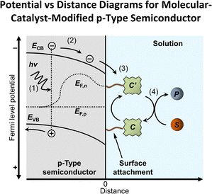 |
| | Fig. 8 A potential versus distance diagram depicting a molecular-catalyst-modified p-type semiconductor interfaced with a solution phase, where (1) photons absorbed by the semiconductor generate electron–hole pairs, (2) charges are separated, and minority carriers in the semiconductor phase (electrons in this example involving a p-type semiconductor) move toward the solution phase, (3) catalysts are activated via interfacial charge transfer (indicated as the conversion of C to C′ in this cartoon diagram), and (4) activated catalysts react with chemical substrates (S) to form chemical products (P). | |
Semiconductor|catalyst interfaces have been classified as Schottky-type “buried junctions” (where the catalyst potential tracks with changes in the applied electrode potential) or as “adaptive junctions” (where the catalyst potential, Ecat, moves independently of the semiconductor potential and band edges).94,107–109 These types of interfaces have been modelled using equivalent circuits (i.e., circuits that are equivalent to the system in the electrochemical cell, comprising electrical components/elements that reflect the effect or contribution to the total impedance) to elucidate the current–potential behavior of semiconductor|catalyst|electrolyte systems.110 If the physical structure of a catalyst is relatively dense or ion-impermeable, as depicted in Fig. 9(a), the catalytic films can give rise to “buried” junctions. Under these conditions, the catalyst layer must accommodate injected charges near the catalyst|electrolyte boundary to achieve charge neutrality by forming a classical double layer within the electrolyte solution phase. This results in an electric potential drop that occurs predominantly across a Helmholtz layer [Fig. 9(b)].80 The barrier height (ϕb, with units of V and defined as the difference between the valence band-edge potential of a p-type semiconductor and the Fermi-level potential of the catalyst layer or the difference between the conduction band-edge potential of a n-type semiconductor and the Fermi-level potential of the catalyst layer)94 shown in Fig. 9(b) thus remains constant between dark and illuminated conditions. The current density produced by buried-semiconductor|dense-catalyst junctions (Jjxn,buried, with units of A cm−2) can be expressed as indicated in eqn (41),
| | | Jjxn,buried = kp(ps − ps0) − kn(ns − ns0) (the current density of buried-semiconductor|dense-catalysts junctions), | (41) |
where
kp is a
forward rate constant for hole transfer between the semiconductor and dense catalyst (with units of A cm), and
kn is a
forward rate constant for electron transfer between the semiconductor and dense catalyst (with units of A cm). Given
kp and
kn are independent of the catalyst potential,
Ecat, the value of
Jjxn,buried is not influenced by or dependent on the value of
Ecat. This is because accumulated charges at the dense catalyst|electrolyte solution interface result in an electric potential drop that appears across the electric double layer without affecting the electric potential across the buried-semiconductor|dense-catalysts junction.
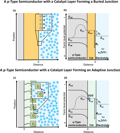 |
| | Fig. 9 (a) Diagram illustrating a p-type semiconductor electrode with a dense catalyst coating layer that is impermeable to electrolyte species in the solution phase and thus forms a “buried” junction, where any charge on the catalyst is balanced by ions forming an electric double layer in the solution phase. (b) A potential versus distance diagram for an illuminated p-type semiconductor with a catalyst layer forming a buried junction, where the barrier height (ϕb), which is the theoretical maximum energy that can be extracted from a separated electron–hole pair, remains unchanged under illuminated versus non-illuminated conditions because the separation between the semiconductor valence band edge (EVB) and the catalyst Fermi level (Ecat) is unchanged. (c) Diagram illustrating a p-type semiconductor electrode with an electrolyte-permeable catalyst coating layer that enables electronic charge on the catalyst to be screened by ions in the solution and thus forms an “adaptive” junction, where there is no electrostatic potential drop across the catalyst layer. (d) A potential versus distance diagram for an illuminated p-type semiconductor with a catalyst layer forming an adaptive junction, where the effective barrier height (ϕb,eff) increases under illumination at a fixed current density due to changes in the concentrations of reduced and oxidized forms of the catalysts and thus variability in the separation between EVB and Ecat. In the catalyst layer, the density of states is abbreviated as DOS. | |
If the physical structure of a catalytic surface coating is ion-permeable—as depicted in Fig. 9(c) and as it can be for molecular catalyst layers and coatings of porous oxide materials—the interfaces are considered “adaptive” junctions. Since the electrocatalyst layer (molecular or other) is permeable to the electrolyte solution, the “adaptive” junctions do not experience an extensive electric potential drop within the catalyst layer, or across the catalyst|electrolyte solution interface. Diffusing ions from the electrolyte solution screen charges, causing the electric potential drop to occur mostly across the space charge region inside the semiconductor [Fig. 9(d)].94,111 Such constructs have been treated as a single semiconductor|catalyst|electrolyte element, and the effective barrier height (ϕb,eff, with units of V and defined as the separation between the valence band-edge potential of a p-type semiconductor and the Fermi level of a catalyst forming an adaptive junction or the separation between the conduction band-edge potential of an n-type semiconductor and the Fermi level of a catalyst forming an adaptive junction)94 changes as a function of Ecat. Because the redox state of the electrocatalyst film is variable, the potential of the catalyst layer moves independently of the semiconductor band positions. Given the potential of the catalyst layer moves independently of the semiconductor band positions, the current density produced by adaptive semiconductor|catalyst junctions (Jjxn,adapt, with units of A cm−2) will depend on the Fermi-level potential difference across the catalyst [Vcat with units of V and defined as the difference between Ecat and the equilibrium potential, Eeq, as indicated in eqn (42)], and can be expressed as indicated in eqn (43),
| | | Vcat = Ecat − Eeq (the Fermi-level potential difference across the catalyst), | (42) |
| | 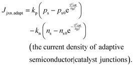 | (43) |
For both ion-impermeable [
Fig. 9(a)] and ion-permeable [
Fig. 9(c)] constructs (
e.g., buried-semiconductor|dense-catalysts junctions and adaptive semiconductor|dense catalysts, respectively), the
current density at the catalyst|electrolyte solution interface (
Jcat, with units of A cm
−2) has been modelled using Butler–Volmer-type kinetics, as expressed in
eqn (44),
| |  | (44) |
Considering both electrons and photons as reactants enables the development of frameworks for extracting kinetic and thermodynamic parameters.94,106,110,112,113 However, as described herein, the interaction of chemical components is physically different from the transfer of charge carriers between (semi)conducting surfaces and electrocatalytic components. Further, the turnover frequency of catalysts operating in photoelectrosynthetic constructs can be limited by the flux of photons. Thus, approaches relevant to benchmarking electrocatalysts can yield erroneous metrics for catalytic components operating in light-activated assemblies if the observed maximum reaction rates are limited by the fluxes of photons rather than the inherent catalytic properties. Applications of wavelength-resolved turnover frequency plots and photoelectrosynthetic Tafel-like plots78 may help identify rate-limiting steps. However, further theory, computational, and experimental efforts are needed to better understand the parallels and differences between molecular catalysts operating in photoelectrosynthetic versus electrocatalytic assemblies.106
VI. Comparing and contrasting kinetics and thermodynamics of conducting versus semiconducting electrodes
Consistent with the Butler–Volmer equation and the Marcus–Hush–Levich theory, and as described in Sections IV and V [see eqn (21)] of this review article, differences in rates of interfacial electron transfer when varying the applied electrode potential, Eapp, of a conducting electrode interfaced with an electrolyte solution are due to changes in the rate constants for heterogeneous electron transfer, arising from the potential-dependent nature of the standard Gibbs free energy of activation for electro-activating the substrates, ΔG‡s. In contrast, differences in rates of interfacial charge transfer when varying the bias potential applied to a semiconducting electrode interfaced with an electrolyte solution can arise from changes in the concentration of minority carriers at the electrode surface as a consequence of the potential-dependent changes in the degree of band bending across the semiconductor space charge region [see eqn (40a) and (40b)]. These differences in charge-transfer kinetics governing the electrochemistry of conducting electrodes versus the photoelectrochemistry of semiconducting electrodes are embodied in the thermodynamic terms depicted in Fig. 10. Consistent with Gibbs free energy relationships and Nernst equations [see eqn (12), (39a) and (39b)], differences in overpotentials involve differences in the relative enthalpic versus entropic (including concentration and electric potential gradients) contributions to the electrochemical driving force.43
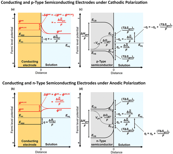 |
| | Fig. 10 (a) and (b) Potential versus distance diagrams depicting conducting working electrodes under cathodic (panel a) or anodic (panel b) biasing of the applied electrode potential (Eapp) relative to the equilibrium potential (Eeq), indicating the related difference in electric potential (Δϕwe) between the electric potential in the working electrode at open-circuit conditions (ϕwe,oc) and following polarization (ϕwe), the Gibbs free energy change associated with polarization of the working electrode (ΔḠpol), the overpotential (η), as well as the Gibbs free energy change for interfacial electron transfer (ΔḠET). (c) and (d) Potential versus distance diagrams depicting an illuminated p-type semiconductor photoelectrode under a cathodic bias (panel c) and an illuminated n-type semiconductor photoelectrode under an anodic bias (panel d), indicating the enthalpy change associated with photon absorption and the generation of electron–hole pairs [ΔHgen, which is related to the band gap of the semiconductor and thus the difference between the conduction band-edge potential (ECB) and valence band-edge potential (EVB) of the semiconductor], the energy loss associated with the mixing entropy terms [(TΔSgen)n and (TΔSgen)p], the difference in Gibbs free energy between the surface quasi-Fermi-level potentials (ΔGgen), the underpotential (ηu), the overpotential (ηo), the intrinsic overpotential (ηi), the Gibbs free energy change for photoinduced charge injection (ΔḠo), and the Gibbs free energy change resulting from an applied electrode potential relative to the equilibrium potential (ΔḠu). | |
In the examples depicted in Fig. 10(a) and (b), involving a conducting electrode, altering the applied electrode potential, Eapp, from the open-circuit potential to an overpotential, η, results in a change in the electric potential in the working electrode (Δϕwe, with units of V) relative to the electric potential in the working electrode at open-circuit conditions (ϕwe,oc, with units of V and defined as the electric potential in the working electrode at open-circuit conditions), as indicated in eqn (45),114,115
| |  | (45) |
where Δ
Ḡpol is the
Gibbs free energy change associated with polarization of the electrode (with units of J mol
−1). The Δ
ϕwe results in an electric potential drop across the electric double layer [as indicated by the changing
ϕsol in Fig. 10(a) and (b)] that mainly appears across the Helmholtz layer. The
Gibbs free energy change for interfacial electron transfer (Δ
ḠET, with units of J mol
−1 and defined as the per-molar difference in Gibbs free energy between the Fermi-level potential of the electrode and the equilibrium potential) the corresponding
enthalpy change for interfacial electron transfer (Δ
![[H with combining macron]](https://www.rsc.org/images/entities/i_char_0048_0304.gif) ET
ET, with units of J mol
–1 and defined as the per-molar difference in enthalpy between the Fermi-level potential of the electrode and the equilibrium potential), as well as
entropy change for interfacial electron transfer (Δ
![[S with combining macron]](https://www.rsc.org/images/entities/i_char_0053_0304.gif) ET
ET, with units of J mol
–1 and defined as the per-molar difference in entropy between the Fermi-level potential of the electrode and the equilibrium potential) are related to
η, as indicated in
eqn (46),
| | | ΔḠET = ΔET − TΔET = F(Eapp − Eeq) = Fη (Gibbs free energy change for interfacial electron transfer). | (46) |
Even under “reversible” conditions, as described in Section II of this review article, an electrochemical process can still involve an entropy change within the system; however, for the universe (system + surroundings), the net entropy change would be zero. In summary, polarizing an electrode creates the electrode potential difference that drives or opposes the interfacial electron transfer process.
In the example depicted in Fig. 10(c), involving a p-type semiconductor photoelectrode, an increase in the semiconductor surface electron concentration, ns, via increased band bending, decreases the mixing entropy for electrons [(TΔSgen)n with units of J mol−1 and defined as the energy loss due to the electrons in the conduction band occupying a fraction of the local density of states at the bottom of the conduction band] as expressed in eqn (47a).95 Increasing the overpotential for a photoelectrochemical reaction with respect to the minority-carrier quasi-Fermi-level potential, ηo, yields an increase in ns, and a related shift of the electron quasi-Fermi-level-potential, EF,n, to higher energies (i.e., more negative potentials), thereby increasing the magnitude of the Gibbs free energy change associated with charge transfer. The Gibbs free energy change for photoinduced charge injection (ΔḠo, with units of J mol−1 and defined as the per-molar difference in Gibbs free energy between the minority carrier's surface quasi-Fermi-level potential and the equilibrium potential) involving p-type semiconductors is thus described viaeqn (48a),
| |  | (47a) |
| | | ΔḠo = F[(EF,n)s − Eeq] = F(ECB − Eeq) + (TΔSgen)n = Fηo (Gibbs free energy change for photoinduced charge injection involving p-type semiconductors). | (48a) |
In the example depicted in
Fig. 10(d), involving an n-type semiconductor photoelectrode, an increase in the semiconductor surface hole concentration,
ps,
via increased band bending, decreases the
mixing entropy for holes [(
TΔ
Sgen)
p with units of J mol
−1 and defined as the energy loss due to the holes in the valence band occupying a fraction of the local density of states at the top of the valence band] as expressed by
eqn (47b).
95 Increasing
ηo yields an increase in
ps, and a related shift of the hole quasi-Fermi-level-potential,
EF,p, to lower energies (
i.e., more positive potentials), thereby increasing the magnitude of the Gibbs free energy change associated with charge transfer. Δ
Ḡo involving n-type semiconductors is thus described
viaeqn (48b),
| |  | (47b) |
| | | ΔḠo = F[(EF,p)s − Eeq] = F(EVB − Eeq) − (TΔSgen)p = Fηo (Gibbs free energy change for photoinduced charge injection involving n-type semiconductors). | (48b) |
In p-type semiconducting electrodes, the intrinsic overpotential (ηi, with units of V and defined as the energy lost via irreversible interfacial charge transfer) is the difference between the conduction band-edge potential and the equilibrium potential (i.e., ECB − Eeq), which is equal to the difference between ηo and the mixing entropy for electrons, (TΔSgen)n, per elementary charge, as indicated in eqn (49a). Alternatively, in n-type semiconducting electrodes, ηi is the difference between the valence band-edge potential and the equilibrium potential (i.e., EVB − Eeq), which is equal to the sum of ηo and the mixing entropy for holes, (TΔSgen)p, per elementary charge, as indicated in eqn (49b),
| |  | (49a) |
| |  | (49b) |
The underpotential for a photoelectrochemical reaction,
ηu, is equated to the
Gibbs free energy change resulting from an applied electrode potential relative to the equilibrium potential (Δ
Ḡu, with units of J mol
−1 and related to the per-molar difference in Gibbs free energy between the majority-carrier's quasi-Fermi-level potential and the equilibrium potential), as indicated in
eqn (50a) and (50b),
| | | ΔḠu = F(EF,p − Eeq) = F(EVB − Eeq) − (TΔSgen)p = Fηu (Gibbs free energy change resulting from an applied electrode potential relative to the equilibrium potential for p-type semiconductors), | (50a) |
| | | ΔḠu = F(EF,n − Eeq) = F(ECB − Eeq) + (TΔSgen)n = Fηu (Gibbs free energy change resulting from an applied electrode potential relative to the equilibrium potential for n-type semiconductors). | (50b) |
As indicated in
eqn (51), the photovoltage,
Vph, is equated to the
difference in Gibbs free energy between surface quasi-Fermi levels (Δ
Ggen, with units of J mol
−1)
via the Faraday constant,
F,
| |  | (51) |
Δ
Ggen can be deconvoluted into corresponding enthalpic and entropic contributions, including the
enthalpy change associated with the photogeneration of electron–hole pairs (Δ
Hgen, with units of J mol
−1 and defined as the enthalpy created by the photon absorption) and the
total entropy of mixing [(
TΔ
Sgen)
mix, with units of J mol
−1 and defined as the sum of mixing entropies for holes and electrons].
95 As further indicated in
eqn (51), the difference between over- and underpotentials,
ηo −
ηu, yields
Vph. Correspondingly, summation of the associated Gibbs free energy changes, −Δ
Ḡo + Δ
Ḡu, is Δ
Ggen.
Kinetic and thermodynamic parameters relevant to charge transfer at conducting and semiconducting electrodes are summarized in Table 2. In conducting electrodes, an applied electrode potential yields an electric potential drop that appears mainly across the Helmholtz layer. In semiconductor electrodes, an applied electrode potential results in an electric potential difference across the space charge region and causes changes in entropic contributions associated with an increase in the photogenerated minority-carrier surface concentration. Applications of the Butler–Volmer equation for describing the kinetics of minority-carrier transfer at semiconductor|electrolyte solution interfaces are likely limited since the energy barrier for interfacial minority-carrier transfer is independent of changes in the quasi-Fermi level.43
Table 2 Parameters associated with the kinetics and thermodynamics of electron/hole transfers at conducting electrodes and semiconducting photoelectrodes
| Electrode type |
Kinetic parameters |
Thermodynamic parameters |
| Conducting |
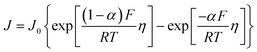
|
η = Eapp − Eeq |
|
|
ΔḠET = F(Eapp − Eeq) = Fη |
|
|
| Semiconducting |
J = Jc + Jv |
For p-type semiconductors |
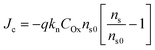
|
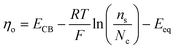
|
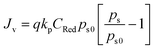
|
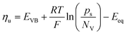
|
|
|
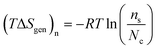
|
|
|
ΔḠo = F(ECB − Eeq) + (TΔSgen)n = Fηo |
|
|
ΔḠu = F(EVB − Eeq) − (TΔSgen)p = Fηu |
|
|
For n-type semiconductors |
|
|
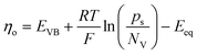
|
|
|
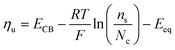
|
|
|
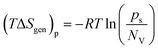
|
|
|
ΔḠo = F(EVB − Eeq) − (TΔSgen)p = Fηo |
|
|
ΔḠu = F(ECB − Eeq) + (TΔSgen)n = Fηu |
VII. Conclusion
In this review of overpotentials and underpotentials in electrochemical versus photoelectrochemical reactions, we also evaluate the enthalpic versus entropic contributions arising from applied electrode potentials. During electrosynthesis involving conducting electrodes, potential-dependent heterogeneous electron-transfer rate constants establish the reaction rates. Differences in overpotential result in changes to the electric potential in the working electrode and an electric potential drop appearing predominantly across the Helmholtz layer of the solution phase. Conversely, during photoelectrosynthesis involving ideal semiconducting electrodes, the reaction rates are predominantly set via potential-dependent degrees of band bending within the electrode phase and the resulting changes in the minority carrier surface concentrations. Here, differences in overpotential result in an electric potential drop appearing predominantly across the space charge region of the working electrode and changes in entropic contributions associated with energy lost by photogenerated charge carriers traversing the space charge region of the semiconductor phase. Nonetheless, in both electrochemical and photoelectrochemical reactions, gradients in electrochemical potentials (a combination of electric and chemical components) ultimately determine reaction spontaneity. Differences in the enthalpic versus entropic contributions to electrosynthesis involving conducting electrodes and photoelectrosynthesis involving semiconducting electrodes could enable novel temperature-dependent strategies for improving efficiencies and advancing applications in artificial photosynthesis and solar-to-fuels technologies.81,116–119 Progress in semiconductor photoelectrochemistry is hampered by limitations of the Butler–Volmer equation to describe the kinetics of minority-carrier transfer at semiconductor photoelectrodes, as well as constraints of the Gerischer model to account for chemically-modified semiconductors and inner-sphere charge-transfer processes.120 We imagine that as new ideas and discoveries continue to emerge, more light will be shed on the concepts reviewed herein.
Author contributions
Daiki Nishiori, Edgar A. Reyes Cruz, Lillian K. Hensleigh, and Nghi P. Nguyen wrote the original draft, reviewed the paper, and edited the paper. Gary F. Moore conceptualized and supervised the project, acquired funding, reviewed the paper, and edited the paper.
Conflicts of interest
The authors declare no competing financial interest.
Data availability
No primary research results, software, or code have been included, and no new data were generated or analyzed as part of this review.
Acknowledgements
This work at Arizona State University (G. F. M.) was supported by the US Department of Energy, Office of Science, Office of Basic Energy Sciences, under Early Career Award DESC0021186 and by the National Science Foundation under Early Career Award 1653982. G. F. M. also acknowledges support from the Camille Dreyfus Teacher-Scholar Awards Program. N. P. N. and D. N. acknowledge support from the Completion Fellowship from the Graduate College, Arizona State University. L. K. H. acknowledges support from the Phoenix Chapter of the ARCS foundation and a Paul Liddell Memorial Synthetic Chemistry Award.
Notes and references
- T. A. Faunce, W. Lubitz, A. W. Rutherford, D. MacFarlane, G. F. Moore, P. Yang, D. G. Nocera, T. A. Moore, D. H. Gregory, S. Fukuzumi, K. B. Yoon, F. A. Armstrong, M. R. Wasielewski and S. Styring, Energy Environ. Sci., 2013, 6, 695–698 RSC.
- S. Ardo, D. Fernandez Rivas, M. A. Modestino, V. Schulze Greiving, F. F. Abdi, E. Alarcon Llado, V. Artero, K. Ayers, C. Battaglia, J. P. Becker, D. Bederak, A. Berger, F. Buda, E. Chinello, B. Dam, V. Di Palma, T. Edvinsson, K. Fujii, H. Gardeniers, H. Geerlings, S. M. Hashemi, S. Haussener, F. Houle, J. Huskens, B. D. James, K. Konrad, A. Kudo, P. P. Kunturu, D. Lohse, B. Mei, E. L. Miller, G. F. Moore, J. Muller, K. L. Orchard, T. E. Rosser, F. H. Saadi, J. W. Schüttauf, B. Seger, S. W. Sheehan, W. A. Smith, J. Spurgeon, M. H. Tang, R. Van De Krol, P. C. K. Vesborg and P. Westerik, Energy Environ. Sci., 2018, 11, 2768–2783 RSC.
- N. S. Lewis, D. G. Nocera and M. P. Nash, Proc. Natl. Acad. Sci. U. S. A., 2006, 103, 15729–15735 CrossRef CAS PubMed.
- J. A. Turner, Science, 1999, 285, 687–689 CrossRef CAS PubMed.
-
A. J. Bard and L. R. Faulkner, Electrochemical methods: fundamentals and applications, John Wiley & Sons, Inc, New York, 2nd edn, 2001 Search PubMed.
- S. W. Boettcher, S. Z. Oener, M. C. Lonergan, Y. Surendranath, S. Ardo, C. Brozek and P. A. Kempler, ACS Energy Lett., 2021, 6, 261–266 CrossRef CAS.
- The units presented for physical quantitites and constants serve as examples and are not universally appied.
-
A. D. McNaught and A. Wilkinson, IUPAC. Compendium of Chemical Terminology. (the ‘Gold Book’), Blackwell Scientific Publications, Oxford, 2nd edn, 1997, vol. 66 Search PubMed.
-
I. N. Levine, Physical Chemistry, McGraw-Hill, New York, 4th edn, 1995 Search PubMed.
- G. N. Lewis, Proc. Am. Acad. Arts Sci., 1907, 43, 259–293 Search PubMed.
-
M. S. Kaufman, Principles of Thermodynamics, CRC Press LLC, New York, 1st edn, 2002 Search PubMed.
-
P. Atkins and J. de Paula, Physical Chemistry, W.H. Freeman, 9th edn, 2010 Search PubMed.
- Fugacity may also be used for condensed phases (liquid or solid), in which case the fugacity a species j in the condensed phase is defined as the fugacity of the vapor phase in equilibrium with the condensed phase (see ref. 12).
-
G. Saville, Activity coefficient. Themopedia, https://www.thermopedia.com/content/288/, (accessed 30 September 2024).
-
V. Hurai, M. Huraiová, M. Slobodník and R. Thomas, in Geofluids: Developments in Microthermometry, Spectroscopy, Thermodynamics, and Stable Isotopes, ed. V. Hurai, M. Huraiová, M. Slobodník and R. Thomas, Elsevier, 2015, pp. 171–230 Search PubMed.
- Although activity coefficients may be used for both liquid and gas phases, conventionally activity coefficients are used for liquid phases and fugacity coefficients for gas phases (see ref. 12).
-
P. Westbroek, G. Priniotakis and P. Kiekens, Analytical electrochemistry in textiles, Woodhead Publishing, 2005, pp. 1–36 Search PubMed.
- G. Jerkiewicz, ACS Catal., 2020, 10, 8409–8417 CrossRef CAS.
- T. Biegler and R. Woods, J. Chem. Educ., 1973, 50, 604–605 CrossRef CAS.
- R. W. Ramette, J. Chem. Educ., 1987, 64, 885 CrossRef CAS.
-
W. Schmickler, E. Santos, W. Schmickler and E. Santos, Interfacial Electrochemistry, Springer, Berlin, Heidelberg, 2010, pp. 29–37 Search PubMed.
-
N. Sato, Electrochemistry at Metal and Semiconductor Electrodes, 1st edn, 1998, pp. 87–117 Search PubMed.
-
E. M. Stuve, in Encyclopedia of Applied Electrochemistry, ed. G. Kreysa, K. Ota and R. F. Savinell, Springer, New York, 2014, pp. 1445–1453 Search PubMed.
- The values of the standard electrode potential,
 , are reported with respect to the SHE for aqueous solutions or the ferrocenium/ferrocene redox system for non-aqueous solutions by convention.
- G. Gritzner and J. Kuta, Pure Appl. Chem., 1984, 56, 461–466 CrossRef.
- The Nernst equation is a thermodynamic relationship applicable under equilibrium conditions. However, when a cell produces a net current, the relationship can still be used to link the electrode potential to the surface concentrations of Ox and Red if the electron transfer kinetics are fast with respect to the mass transfer kinetics. Under these conditions, the electrode potential and the surface concentrations are kept in equilibrium with each other by the relatively fast charge-transfer processes even though the surface concentrations are not in equilibrium with the bulk (see ref. 5).
- S. U. M. Khan, R. C. Kainthla and J. O. M. Bockris, J. Phys. Chem., 1987, 91, 5974–5977 CrossRef CAS.
-
R. Memming, Semiconductor Electrochemistry, John Wiley & Sons, Inc, 2nd edn, 2015, pp. 49–64 Search PubMed.
- S. Fletcher, J. Solid State Electrochem., 2020, 24, 3029–3038 Search PubMed.
- In eqn (16), ϕsol is expressed with units of volts versus a reference electrode, and thus, the ϕref term is included to account for this.
- F. A. Armstrong and J. Hirst, Proc. Natl. Acad. Sci. U. S. A., 2011, 108, 14049–14054 CrossRef CAS PubMed.
- C. F. Wise, R. G. Agarwal and J. M. Mayer, J. Am. Chem. Soc., 2020, 142, 10681–10691 Search PubMed.
-
R. Memming, Semiconductor Electrochemistry, John Wiley & Sons, Inc, 2nd edn, 2015, pp. 169–266 Search PubMed.
- L. Chen, Q. Chen, C. Wang and Y. Li, J. Am. Chem. Soc., 2020, 142, 18281–18292 Search PubMed.
-
N. Sato, Electrochemistry at Metal and Semiconductor Electrodes, Elsevier B.V., 1st edn, 1998, pp. 119–199 Search PubMed.
- E. E. Barton, D. M. Rampulla and A. B. Bocarsly, J. Am. Chem. Soc., 2008, 130, 6342–6344 CrossRef CAS PubMed.
- A. Krawicz, J. Yang, E. Anzenberg, J. Yano, I. D. Sharp and G. F. Moore, J. Am. Chem. Soc., 2013, 135, 11861–11868 Search PubMed.
- T. P. Senftle, M. Lessio and E. A. Carter, ACS Cent. Sci., 2017, 3, 968–974 CrossRef CAS PubMed.
- B. M. Stratakes and A. J. M. Miller, ACS Catal., 2020, 10, 9006–9018 CrossRef CAS.
- R. Parsons, Pure Appl. Chem., 1979, 52, 233–240 Search PubMed.
- M. C. Henstridge, E. Laborda, N. V. Rees and R. G. Compton, Electrochim. Acta, 2012, 84, 12–20 CrossRef CAS.
- J. O. Bockris and Z. Nagy, J. Chem. Educ., 1973, 50, 839–843 Search PubMed.
- L. M. Peter, J. Solid State Electrochem., 2013, 17, 315–326 CrossRef CAS.
-
D. K. Gosser Jr., Cyclic Voltammetry; Simulation and Analysis of Reaction Mechanisms, Wiley-VCH, New York, 1993 Search PubMed.
- J. Tafel, Z. Phys. Chem., 1905, 50A, 641–712 Search PubMed.
- K. J. Laidler, Pure Appl. Chem., 1996, 68, 149–192 CrossRef CAS.
- L. Wei, N. Tian, Z. Y. Zhou, Y. X. Jiang and S. G. Sun, Encycl. Interfacial Chem. Surf. Sci. Electrochem., 2018, 507–520 Search PubMed.
- Z. W. She, J. Kibsgaard, C. F. Dickens, I. Chorkendorff, J. K. Nørskov and T.
F. Jaramillo, Science, 2017, 355, eaad4998 Search PubMed.
- R. H. Crabtree, Chem. Rev., 2012, 112, 1536–1554 CrossRef CAS PubMed.
- M. N. Jackson, C. J. Kaminsky, S. Oh, J. F. Melville and Y. Surendranath, J. Am. Chem. Soc., 2019, 141, 14160–14167 CrossRef CAS.
- M. N. Jackson, M. L. Pegis and Y. Surendranath, ACS Cent. Sci., 2019, 5, 831–841 Search PubMed.
- M. N. Jackson and Y. Surendranath, Acc. Chem. Res., 2019, 52, 3432–3441 CrossRef CAS PubMed.
- J.-M. Savéant, Chem. Rev., 2008, 108, 2348–2378 CrossRef PubMed.
- M. N. Jackson, O. Jung, H. C. Lamotte and Y. Surendranath, ACS Catal., 2019, 9, 3737–3743 CrossRef CAS.
- C. J. Kaminsky, S. Weng, J. Wright and Y. Surendranath, Nat. Catal., 2022, 5, 430–442 CrossRef CAS.
- P. Hutchison, C. J. Kaminsky, Y. Surendranath and S. Hammes-Schiffer, ACS Cent. Sci., 2023, 9, 927–936 Search PubMed.
- W. Nie and C. C. L. McCrory, Dalton Trans., 2022, 51, 6993–7010 Search PubMed.
- S. W. Feldberg, Anal. Chem., 2010, 82, 5176–5183 Search PubMed.
-
A. A. Balandin, Advances in Catalysis, ed. D. D. Eley, H. Pines and P. B. Weisz, Academic Press, 1969, vol. 19, pp. 1–210 Search PubMed.
- P. Sabatier, Berichte der Dtsch. Chem. Gesellschaft, 1911, 44, 1984–2001 Search PubMed.
- J. Kari, J. P. Olsen, K. Jensen, S. F. Badino, K. B. R. M. Krogh, K. Borch and P. Westh, ACS Catal., 2018, 8, 11966–11972 Search PubMed.
- T. Bligaard, J. K. Nørskov, S. Dahl, J. Matthiesen, C. H. Christensen and J. Sehested, J. Catal., 2004, 224, 206–217 Search PubMed.
- C. Costentin and J.-M. Savéant, ACS Appl. Mater. Interfaces, 2017, 9, 19894–19899 CrossRef CAS PubMed.
- T. Shinagawa, A. T. Garcia-Esparza and K. Takanabe, Sci. Rep., 2015, 5, 1–21 Search PubMed.
- R. Guidelli, R. G. Compton, J. M. Feliu, E. Gileadi, J. Lipkowski, W. Schmickler and S. Trasatti, Pure Appl. Chem., 2014, 86, 245–258 Search PubMed.
-
R. H. Crabtree, in The Organometallic Chemistry of the Transition Metals, ed. R. H. Crabtree, Wiley, 2014, pp. 224–258 Search PubMed.
- T. Bligaard, R. M. Bullock, C. T. Campbell, J. G. Chen, B. C. Gates, R. J. Gorte, C. W. Jones, W. D. Jones, J. R. Kitchin and S. L. Scott, ACS Catal., 2016, 6, 2590–2602 Search PubMed.
- J. M. Pingarrón, J. Labuda, J. Barek, C. M. A. Brett, M. F. Camões, M. Fojta and D. B. Hibbert, Pure Appl. Chem., 2020, 92, 641–694 CrossRef.
- E. J. Piechota and G. J. Meyer, J. Chem. Educ., 2019, 96, 2450–2466 CrossRef CAS.
- V. Artero and J.-M. Savéant, Energy Environ. Sci., 2014, 7, 3808–3814 RSC.
- C. Costentin and J.-M. Savéant, ChemElectroChem, 2014, 1, 1226–1236 CrossRef CAS.
- E. S. Rountree, B. D. McCarthy, T. T. Eisenhart and J. L. Dempsey, Inorg. Chem., 2014, 53, 9983–10002 Search PubMed.
- C. Costentin, S. Drouet, M. Robert and J.-M. Savéant, J. Am. Chem. Soc., 2012, 134, 11235–11242 Search PubMed.
- C. Costentin and J.-M. Savéant, Nat. Rev. Chem., 2017, 1, 87 CrossRef CAS.
- F. Calle-Vallejo, Appl. Phys. Rev., 2024, 11(2), 021305 CAS.
- L. Pauling, Nature, 1948, 161, 707–709 Search PubMed.
- T. L. Amyes and J. P. Richard, Biochemistry, 2013, 52, 2021–2035 Search PubMed.
- D. Nishiori, L. K. Hensleigh, N. P. Nguyen, I. Peterson and G. F. Moore, ACS Catal., 2025, 15, 6361–6371 Search PubMed.
- A. J. Bard, R. Memming and B. Miller, Pure Appl. Chem., 1991, 63, 569–596 Search PubMed.
- A. C. Nielander, M. R. Shaner, K. M. Papadantonakis, S. A. Francis and N. S. Lewis, Energy Environ. Sci., 2015, 8, 16–25 Search PubMed.
- E. A. Reyes Cruz, D. Nishiori, B. L. Wadsworth, N. P. Nguyen, L. K. Hensleigh, D. Khusnutdinova, A. M. Beiler and G. F. Moore, Chem. Rev., 2022, 122, 16051–16109 Search PubMed.
- J. Bisquert, P. Cendula, L. Bertoluzzi and S. Gimenez, J. Phys. Chem. Lett., 2014, 5, 205–207 Search PubMed.
- A. J. Bard, J. Photochem., 1979, 10, 59–75 Search PubMed.
- A. Heller, Acc. Chem. Res., 1981, 14, 154–162 Search PubMed.
- F. E. Osterloh, ACS Energy Lett., 2017, 2, 445–453 CrossRef CAS.
-
W. Plieth, in Electrochemistry for Materials Science, ed. W. Plieth, Elsevier, 1st edn, 2008, pp. 27–69 Search PubMed.
-
C. Kittel, Introduction to Solid State Physics, John Wiley & Sons, Inc, 8th edn, 2004 Search PubMed.
-
K. Rajeshwar, Encyclopedia of Electrochemistry, Wiley Online Library, 2007 Search PubMed.
- F. Williams and A. J. Nozik, Nature, 1984, 312, 21–27 Search PubMed.
- M. G. Walter, E. L. Warren, J. R. McKone, S. W. Boettcher, Q. Mi, E. A. Santori and N. S. Lewis, Chem. Rev., 2010, 110, 6446–6473 CrossRef CAS PubMed.
-
R. van de Krol, in Photoelectrochemical Hydrogen Production, ed. R. van de Krol and M. Grätzel, Springer US, Boston, MA, 2012, pp. 13–68 Search PubMed.
-
N. Sato, Electrochemistry at Metal and Semiconductor Electrodes, Elsevier B.V., 1st edn, 1998, pp. 325–371 Search PubMed.
-
L. M. Peter, in Photocatalysis: Fundamentals and Perspectives, ed. J. Schneider, D. Bahnemann, J. Ye, G. L. Puma and D. D. Dionysiou, Royal Society of Chemistry, 2016, pp. 1–28 Search PubMed.
- M. R. Nellist, F. A. L. Laskowski, F. Lin, T. J. Mills and S. W. Boettcher, Acc. Chem. Res., 2016, 49, 733–740 Search PubMed.
- P. Salvador, J. Phys. Chem. B, 2001, 105, 6128–6141 CrossRef CAS.
- M. Schleuning, I. Y. Ahmet, R. van de Krol and M. M. May, Sustainable Energy Fuels, 2022, 6, 3701–3716 RSC.
- T. Hannappel, S. Shekarabi, W. Jaegermann, E. Runge, J. P. Hofmann, R. van de Krol, M. M. May, A. Paszuk, F. Hess, A. Bergmann, A. Bund, C. Cierpka, C. Dreßler, F. Dionigi, D. Friedrich, M. Favaro, S. Krischok, M. Kurniawan, K. Lüdge, Y. Lei, B. Roldán Cuenya, P. Schaaf, R. Schmidt-Grund, W. G. Schmidt, P. Strasser, E. Unger, M. F. Vasquez Montoya, D. Wang and H. Zhang, Sol. RRL, 2024, 8, 2301047 CrossRef CAS.
- A. J. Bard, A. B. Bocarsly, F. F. Fan, E. G. Walton and M. S. Wrighton, J. Am. Chem. Soc., 1980, 102, 3671–3677 CrossRef CAS.
- K. W. Frese and S. R. Morrison, J. Electrochem. Soc., 1979, 126, 1235–1241 Search PubMed.
- P. Allongue and H. Cachet, J. Electrochem. Soc., 1985, 132, 45–52 CrossRef CAS.
- D. Lincot and J. Vedel, J. Electroanal. Chem., 1987, 220, 179–200 CrossRef CAS.
- N. D. Keller, P. Vecchi, D. C. Grills, D. E. Polyansky, G. P. Bein, J. L. Dempsey, J. F. Cahoon, G. N. Parsons, R. N. Sampaio and G. J. Meyer, J. Am. Chem. Soc., 2023, 145, 11282–11292 CrossRef CAS PubMed.
- J. Reichman, Appl. Phys. Lett., 1980, 36, 574–577 CrossRef CAS.
- H. Gerischer, J. Electroanal. Chem. Interfacial Electrochem., 1975, 58, 263–274 Search PubMed.
- L. M. Peter, Chem. Rev., 1990, 90, 753–769 CrossRef CAS.
- D. Nishiori, B. L. Wadsworth and G. F. Moore, Chem. Catal., 2021, 1, 978–996 CAS.
- R. H. Walden, R. H. Krambeck, R. J. Strain, J. McKenna, N. L. Schryer and G. E. Smith, Bell Syst. Tech. J., 1972, 51, 1635–1640 Search PubMed.
- S. W. Boettcher, E. L. Warren, M. C. Putnam, E. A. Santori, D. Turner-Evans, M. D. Kelzenberg, M. G. Walter, J. R. McKone, B. S. Brunschwig, H. A. Atwater and N. S. Lewis, J. Am. Chem. Soc., 2011, 133, 1216–1219 CrossRef CAS PubMed.
- F. Lin and S. W. Boettcher, Nat. Mater., 2014, 13, 81–86 Search PubMed.
- T. J. Mills, F. Lin and S. W. Boettcher, Phys. Rev. Lett., 2014, 112, 148304 Search PubMed.
- F. Lin, E. M. Walker and M. C. Lonergan, J. Phys. Chem. Lett., 2010, 1, 720–723 Search PubMed.
- W. Li, D. He, S. W. Sheehan, Y. He, J. E. Thorne, X. Yao, G. W. Brudvig and D. Wang, Energy Environ. Sci., 2016, 9, 1794–1802 RSC.
- B. L. Wadsworth, A. M. Beiler, D. Khusnutdinova, E. A. Reyes Cruz, G. F. Moore, E. A. R. Cruz and F. Gary, J. Am. Chem. Soc., 2019, 141, 15932–15941 Search PubMed.
- J. E. B. Randles, Faraday Discuss., 1947, 1, 11–19 Search PubMed.
- E. R. Larios-Durán and M. Bárcena-Soto, J. Solid State Electrochem., 2024, 28, 995–1006 CrossRef.
- M. Kölbach, K. Rehfeld and M. M. May, Energy Environ. Sci., 2021, 14, 4410–4417 RSC.
- N. P. Nguyen and G. F. Moore, Joule, 2021, 5, 2254–2256 CrossRef.
- M. A. Modestino and S. Haussener, Annu. Rev. Chem. Biomol. Eng., 2015, 6, 13–34 CrossRef CAS PubMed.
- F. E. Osterloh, J. Phys. Chem. Lett., 2014, 5, 3354–3359 CrossRef CAS PubMed.
- J. B. Sambur, A. J. Kaufman, A. Montoya-Castillo, A. Kundman, A. J. Nozik, A. G. DesCarpentrie, A. Jana, A. Tews, A. Banik, B. C. M. Martindale, B. DeBruine, B. A. Parkinson, C. D. Frisbie, C. Tossi, C. D. Hallock, D. V. Esposito, D. R. Lustig, D. Ingram, D. Seo, D. Solanki, D. Wang, E. L. Ratcliff, F. A. Houle, F. M. Toma, G. Zhu, G. F. Moore, G. J. Meyer, H. Liu, H. Begum, J. Schneidewind, J. F. Cahoon, J. M. Mayer, J. R. Brinker, J. L. Dempsey, J. Mendes, J. Diederich, J. N. Hart, K. Brinkert, K. Rajeshwar, K.-S. Choi, L. A. Berben, M. Salvi, M. T. Spitler, M. J. Rose, N. S. Lewis, N. A. Gomez, O. Maurya, P. O. Aghadiuno, P. V. Kamat, R. C. Evans, R. Almaraz, R. N. Sampaio, R. H. Coridan, R. van de Krol, S. Suo, S. V. Magpantay, S. Bae, S. K. Cushing, S. Ardo, S. W. Boettcher, S. Hu, S. Maldonado, T. Liu, T. Cuk, T. Hannappel, T. Sayer, T. Arthur, T. G. Deutsch, V. Streibel, W. D. H. Stinson, W. Jaegermann, Y. Surendranath, Z. Mi and Z. Ye, ACS Energy Lett., 2025, 10, 6578–6595 CrossRef CAS.
|
| This journal is © The Royal Society of Chemistry 2026 |
Click here to see how this site uses Cookies. View our privacy policy here. 

 ,
Edgar A.
Reyes Cruz
,
Edgar A.
Reyes Cruz




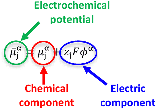

 with units of J mol−1 and defined as the chemical potential of the species j in phase α in the standard state (i.e., the state of a system chosen as a standard for reference by convention8)], the universal gas constant (R, which is exactly 8.31447261815324 J K−1 mol−1), and the chemical activity of a speciesjin phaseα (aαj, a dimensionless quantity defined as the thermodynamic concentration accounting for non-ideal behavior arising from intermolecular interactions between all species present in the solution).9,10


 represents the integral of the dot product of the electric field intensity,
  and the electrochemical potential of H+ in the solution phase
  is set to zero. Thus, a Pt electrode in equilibrium (i.e., where the rates of forward and reverse reactions are equal and no net reaction takes place) with H2 and H+ at unit activities would have an electrochemical potential of electrons in platinum (


 , with units of V vs. a defined reference state and defined as the electrode potential of a half-reaction under standard conditions), as expressed in eqn (12),5,8,24,25
 or the fugacity of H2 in the gas phase
  is not required to be at standard conditions]. The reversible hydrogen electrode potential (ERHE, with units of V vs. Eref and defined as the Fermi-level potential of the reversible hydrogen electrode) is equated to the standard hydrogen electrode potential (ESHE, with units of V vs. Eref and defined as the standard electrode potential for the proton reduction half-reaction) via the Nernst relationship, as shown in eqn (13),18
 . The pH of a solution is expressed as a function of
  , as indicated in eqn (14),
 , with units of V vs. Eref and defined as the reduction potential of the half-reaction when the oxidized and reduced forms of chemical species, Ox and Red, respectively, are present in the solution phase at concentrations such that the ratio, CsolOx/CsolRed, is unity, but other substances—such as protons or other specified species—can be present at designated, non-standard conditions).5 Formal potentials are expressed using the chemical activity coefficients of Ox and Red in the solution phase (γsolOx and γsolRed, respectively), as indicated in eqn (15),

 , and the chemical activities of Ox and Red in the solution phase (asolOx and asolRed, respectively), as expressed in the modified Nernst equation (including the addition of the ϕsol and ϕref terms) shown in eqn (17),6,27–29
 and
and  , respectively) set the equilibrium potential (Eeq, with units of V vs. Eref and defined as the Fermi-level potential of the solution phase determined from an applied electrode potential at which no net current flows). Thus, Eeq is equivalent in value to the open-circuit potential (Eoc, with units of V vs. Eref) established by the solution mixture when both Ox and Red are present in the solution phase and there are no contributions from liquid junctions.5,31,32 This relationship is expressed in eqn (18),
 is the electrochemical potential of electrons in the bulk solution,
  and
and  are concentrations of Ox and Red in the bulk solution. Unlike Esol (which can be position-dependent with respect to the distance from the electrode surface and is defined by the position-dependent asolOx and asolRed), Eeq is defined under equilibrium conditions and thus is not position-dependent.6,33 Nonetheless, at equilibrium (i.e., where
  (and thus the Fermi-level potential of the working electrode, Ewe, and the equilibrium potential, Eeq), can differ in value [Fig. 2(a)]. Following contact, and upon equilibration,
  (and thus Ewe and Eeq) will become spatially and temporally equal in value [Fig. 2(b)]. Any additional charge that forms on the electrode surface during equilibration is balanced by the ionic charge (with units of C and defined as the charge carried by ions) in the solution phase, where the charge is equal in magnitude to the charge on the working electrode but carries the opposite charge sign (i.e., net positive or negative in charge). As indicated in Fig. 2(b), the concentration gradient of ions in the solution phase forms the electric double layer (EDL), which is an array of charged species and oriented electric dipole moments (


 is the standard heterogeneous electron transfer rate constant (with units of m s−1, yet commonly reported with units of cm s−1, and defined as the value of heterogeneous electron transfer rate constants of the anodic and cathodic reactions under standard conditions).5,40 Thus, under standard conditions, and when the working electrode potential, Ewe, is equilibrated with the equilibrium potential, Eeq, of the solution phase [see Fig. 2(b)], the values of kETa, kETc, and
  are equivalent. Further, for electron transfer reactions involving conducting electrodes, the concentration of electrons in the electrode phase is effectively constant and independent of the applied electrode potential. Changes in overpotential do, however, alter the activation energy (due to the electric potential dropping across the EDL) and hence the rate constants for electron transfer.43
 and
and  . Correspondingly, the solution potential at the electrode surface, (Esol)s, will be approximately equal to the equilibrium potential [i.e., across the solution phase Esol ≈ Eeq and thus (Esol)s ≈ Eeq, as illustrated in Fig. 2(c) and (d)]. Under such conditions, the current density (J, with units of A cm−2 and defined as the amount of charge flowing through a cross-section perpendicular to the flow per unit cross-sectional area and unit time)8 can be described using the form of the Butler–Volmer equation shown in eqn (21),

 values ∼< 3.0 × 10⁻⁵ cm s−1). Under these conditions the reaction is termed electrochemically irreversible and any applied overpotential, η, is dominated by kinetic overpotential [ηkin, with units of V and defined as the difference between Eapp and (Esol)s as expressed by eqn (23), which is the component of the overpotential required to overcome the activation energy for heterogeneous electron transfer] [see Fig. 2(c) and (d)],
 values ∼> 0.020 cm s−1). Further, any applied η will be dominated by concentration overpotential [ηconc, with units of V and defined as the difference between (Esol)s and Eeq as expressed by eqn (24), which is the component of the overpotential associated with changing the surface concentrations of chemical substrates] [see Fig. 2(e) and (f)],
 ), the reaction is termed electrochemically quasi-reversible. Since J0 is larger than that of an electrochemically irreversible reaction, both anodic and cathodic processes contribute to the net current.5 At relatively lower overpotentials, the net currents will be predominantly limited by heterogeneous electron transfer. Conversely, at relatively higher overpotentials, the net currents will be predominantly limited by mass transport. Thus, under electrochemically quasi-reversible conditions, the applied η is the sum of ηkin and ηconc, as indicated in eqn (25) [see Fig. 2(g) and (h)],
 values relating to definitions of electrochemical reversibility is summarized in Table 1. Although not detailed in this article, there are extended forms of the Butler–Volmer equation that account for mass transport limitations and describe the diffusion-limited region of current–overpotential curves.5 Further details on the Tafel equations, including their applications in the benchmarking of catalysts are covered in the subsequent Section III on overpotentials in electrocatalysis.


 represent applied electrode potentials, ΔḠ‡s and
  represent changes in standard Gibbs free energy of activation for forming a catalyst–substrate reaction intermediate, and
  and
and  represent changes in standard Gibbs free energy for forming a catalyst–substrate reaction intermediate at the respective applied electrode potentials of Eapp or
  . Individual electron transfer or intermediate steps are not depicted for simplicity. (d) A mechanistic scheme involving interfacial outer-sphere electron transfer between an electrode and a homogeneous molecular catalyst (C). (e) A Fermi-level potential versus distance diagram depicting a conducting electrode|homogeneous catalyst solution interface, where catalysis proceeds through outer-sphere electron transfer. A negative polarization of the working electrode increases the driving force for outer-sphere electron transfer from the electrode to the catalyst, whereas the driving force for substrate activation (ηeff) is determined by the standard reduction potential of the catalyst
  and is independent of the applied potential. (f) A Gibbs free energy diagram illustrating an electrocatalytic reduction proceeding via an outer-sphere electron transfer mechanism, where C is activated via electron transfer to form an activated form of the catalyst (C′), which further reacts with a S to form a catalyst–substrate reaction intermediate (C–S). ΔḠ‡ET and
  are changes in standard Gibbs free energy of activation for interfacial electron transfer from the electrode to the catalyst at applied electrode potentials of Eapp or
  , respectively, and
  and
and  are the changes in standard Gibbs free energy for interfacial electron transfer from the electrode to the catalyst at applied electrode potentials of Eapp or
  . Only the highest-energy barriers for the electron transfer and substrate activation are depicted for simplicity. Although the figures illustrate cathodic reactions, related concepts apply to anodic reactions, where positive polarization of the working electrode increases the driving force for activating chemical substrates in the bulk solution (via inner-sphere mechanisms) or the driving force for activating the homogeneous catalysts (via outer-sphere mechanisms) to increase the rate of oxidation reactions.
 , as shown in eqn (26),
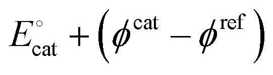 in eqn (26), shift in response to changes in the bias potential.50–52,55,56 When the heterogeneous catalytic sites are part of—and thus integral to—a working electrode, the Fermi-level potentials of the working electrode, Ewe, and the catalysts, Ecat, will track with each other when biasing the working electrode. Thus, polarizing the working electrode with respect to a reference electrode will not provide additional driving force for electron transfer between the working electrode and the catalysts [see Fig. 4(b) depicting an example involving a cathodic reaction]. Polarizing the working electrode does however alter the magnitude of the electric potential drop across the EDL.50,52,55–57
 , as indicated in Fig. 4(c), increases the magnitude of the standard Gibbs free energy change for forming the catalyst–substrate reaction intermediate [indicated as
  and
and  in Fig. 4(c), with units of J mol−1 and defined as the Gibbs free energy change associated with formation of the catalyst–substrate reaction intermediate].50 Consistent with the Butler–Volmer equation and Marcus–Hush–Levich theory,41,44,58 in addition to setting the thermodynamic driving force for the electron-transfer reaction, the overpotential also influences the electrochemical reaction kinetics by modulating the potential-dependent change in standard Gibbs free energy of activation for forming a catalyst–substrate reaction intermediate [indicated as ΔḠ‡s and
  in Fig. 4(c), with units of J mol−1 and defined as the Gibbs free energy required to form the transition state structure]. Nonetheless, the overpotential is a thermodynamic parameter.


 , with units of V vs. Eref and representative of the electrode potential where half of the total number of catalysts (C + C′) at the interface of the electrode and catalyst-containing electrolyte solution are present in their activated form, C′] does not track with the applied electrode potential, Eapp, and instead remains constant in value. As indicated in eqn (29), the difference between the equilibrium potential, Eeq, and
  sets the value of the effective overpotential (ηeff, with units of V),
 , providing further driving force8,69 for activating the catalyst.
 , as indicated in Fig. 4(f), increases the magnitude of the potential-dependent standard Gibbs free energy change for electron transfer from the electrode to the catalyst [
 or
or  in Fig. 4(f), with units of J mol−1 and defined as the difference in standard Gibbs free energy between the reactant state (i.e., prior to interfacial electron transfer) and the product state (i.e., following interfacial electron transfer)].50,52,55 In general, a cathodic biasing of Eapp for a reductive electrochemical transformation also lowers the change in standard Gibbs free energy of activation for electron transfer from the electrode to the catalyst [indicated as
  and
and  in Fig. 4(f), with units of J mol−1 and defined as the difference in standard Gibbs free energy between the reactant state and transition state structures associated with the electron transfer]. However, as opposed to heterogeneous catalysis, polarizing the working electrode does not alter the thermodynamics of chemical steps associated with catalyst–substrate binding when the electron transfer and catalyst–substrate binding proceed via stepwise mechanisms rather than concerted pathways. The standard Gibbs free energy change for forming a catalyst–substrate reaction intermediate,
  , consequently, does not change when modulating Eapp. By extension, changing the value of Eapp does not influence the standard Gibbs free energy of activation for forming a catalyst–substrate reaction intermediate,
  in Fig. 4(f). Thus, under an appropriate bias, the maximum reaction rate can become independent of Eapp and limited by kinetics associated with chemical catalysis.57

 to form an enzyme-substrate complex, indicating the relatively high specificity of enzymes for binding an “activated complex.” Panels a and b were adapted with permission from Nishiori et al., 2021. Copyright 2021 Chemical Catalysis.





