Applying R-matrix theory to atom–molecule inelastic collisions: the case study of H2O + H
Received
20th November 2025
, Accepted 15th December 2025
First published on 16th December 2025
Abstract
The present study presents a comprehensive theoretical investigation of atom and asymmetric top molecule inelastic scattering based on the R-matrix formalism. The proposed methodology establishes a rigorous framework for treating inelastic collisions in the space-fixed coordinate system. The excellent numerical performance of the method is demonstrated through the comparison of state-to-state rotationally inelastic R-matrix cross sections for the H + H2O system with those obtained using conventional close-coupling (CC) theory. The R-matrix approach is shown to deliver results of comparable accuracy while achieving substantially reduced computation times. The method is furthermore shown to achieve more than one order-of-magnitude speedup by exploiting GPU-accelerated diagonalisation through the MAGMA library. This combination of accuracy and computational efficiency positions the R-matrix approach as a powerful and scalable tool for investigating inelastic scattering involving complex polyatomic systems, thereby paving the way for systematic studies of molecule–molecule interactions in astrophysical, atmospheric, and cold-matter environments.
1 Introduction
Inelastic collisions between atoms and molecules or between two molecules play a central role in a wide range of environments, from interstellar1 to circumstellar media,2 planetary atmospheres,3 plasmas4 and combustion systems.5 Accurate quantum mechanical data for such processes are therefore essential in many fields. The prevailing state of the art for modelling inelastic scattering is the close-coupling (CC) method,6 which treats all the degrees of freedom by solving the Schrödinger equation of the system. While the CC method offers highly accurate results and has been validated with state-of-the-art experiments, its computational cost becomes prohibitively high as the numbers of molecular degrees of freedom and scattering channels increase. Approximations such as the coupled states (CS),7 infinite order sudden approximation (IOSA)8 or near neighbours CS (NNCS)9 alleviate the cost but often fail to describe resonance features of threshold effects with sufficient accuracy.
Originally developed in the middle of the twentieth century to address nuclear physics collision problems,10,11 the R-matrix theory offers an appealing alternative framework for dealing with such issues. Later, it was very successfully extended outside nuclear physics to a large class of problems involving electron collision with atoms12 or molecules,13 which became its favorite playground. The fundamental concept of the method is based on the division of the molecular configuration space into three regions: an inner region comprising all short-range interactions, an outer region where long-range interactions predominate and where propagation to the asymptotic region can be conducted efficiently, and a final asymptotic region where the interaction potential is negligible and the matching to asymptotic boundary conditions can be performed to extract all the physical information of the collision.
The R-matrix theory14 is distinguished by its ability to convert a scattering problem into a calculation of molecular states enclosed in an (hyper)spherical box of finite radius. This enables the highly efficient tools developed by the electronic structure community over many years to be used to solve the latter problem independently of the collision energy. The ratio of the scattering wave function divided by its derivative (i.e. the R matrix) at the inner region boundary is then obtained at any collision energy from these box-state energies and wave functions in a very simple and extremely fast way. It is then propagated into the outer region up to the asymptotic boundary by using any of the usual R-matrix propagators.15,16 Alternatively, it can be inverted to obtain the log-derivative matrix at the boundary and propagated using the log-derivative propagators.17–19 This propagation is necessary in the case of electron–molecule collisions since the charge–dipole (or charge-induced dipole) interaction generates a very long range potential. In the present case of collisions between heavy neutral colliders, the long range potential is decreasing a lot faster and we will see that the R-matrix calculated at the boundary of the inner region allows obtaining K matrices undistinguishable from the CC one, thus circumventing the propagation in the outer region.
The R-matrix theory adds a Bloch operator20 to the molecular Hamiltonian. The sum of both operators is hermitian in the box while it is not the case of the Hamiltonian alone. Furthermore, this enforces the continuity of the wave function derivative at the boundary of the box. This effectively transforms a scattering propagation problem into an eigenvalue problem, a class of problems that has been studied intensively in quantum chemistry for over fifty years, leading to highly optimized and efficient numerical methods. Solving the inner-region problem is still computationally demanding, both in terms of CPU time and memory usage. However, it only needs to be performed once for each value of the total angular momentum and a given symmetry of the system (parity, exchange of identical particles…). A further advantage is that GPU-accelerated algebra libraries, such as the NVIDIA Math Libraries21 or MAGMA,22 can be employed to handle large diagonalization tasks efficiently.
While the R-matrix theory has been successfully used in the field of electron-atom/molecule collisions13,14 and nuclear physics,23,24 only a few attempts have been made to apply it to atomic and molecular collisions. Pioneering work was conducted in the 1980s, when Bocchetta and Gerratt applied the method to a 2D model atom–diatom collision problem25 and later to an atom-asymmetric top collision problem.26 Unfortunately, these first studies did not receive much attention within the dynamicist community, most likely because memory was so expensive at that time. The latter study used a very simple model potential, was constrained to a limited energy interval and solely 10 partial waves. The conclusion drawn was that the R-matrix method was incapable of reproducing certain CC resonances because of the strong limitations of the computer facilities at that time. The Tennyson group recently made a new attempt to popularise the method within the ultra cold collisions community27 by demonstrating its application to elastic Ar–Ar scattering, first with a Morse potential28 and later using several ab initio potential energy curves.29 The same team then proposed a roadmap for extending its application domain to multiple physical processes in atom–diatom collisions.30
In this study, we present a comprehensive application of R-matrix theory to inelastic collisions involving an atom and a rotating asymmetric top (RAST) molecule, as exemplified by the collision between atomic hydrogen and rigid water molecule. This system is an ideal benchmark thanks to its astrophysical and atmospheric importance, and to the wealth of previous theoretical studies based on CC method. It furthermore offers a rich physics arising from the strong anisotropy of the H + H2O interaction potential and the large number of accessible rotational states of H2O. It is also typical of systems that require the rotational basis set to be limited, as well as other degrees of freedom such as the vibrational bending motion, and to neglect remaining degrees of freedom, such as the vibrational stretching, in order to avoid an overwhelming increase of the size of the CC calculations.
In the Methods section, we first provide details of how the R-matrix approach is implemented to treat this system. In the Calculation section, we detail the parameters used for the R-matrix calculations. In the Results and discussion section, the H + H2O box-state energies are computed using three different Lagrange Mesh basis of the radial coordinate and compared. The R-matrix method ability to describe intricate resonance patterns and thresholds is then investigated by comparing with available CC results. The computer time performances of the two methods are also compared and the R-matrix scalability is eventually discussed in the section.
2 Methods
2.1 R-matrix theory
Two different versions of the R-matrix exist and have been widely used in the fields of nuclear, atomic, and molecular physics.24 The first one, known as the phenomenological R-matrix, aims to parametrise scattering data such as resonance widths and energies. The second one, known as the calculable R-matrix, which is the one used in this work, aims to accurately solve the Schrödinger equation, mainly for scattering problems, but it can be also useful for bound state calculations in the case of very shallow potential well and in the case of a very long-range potential for the states just below the dissociating limit.
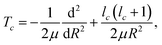
To introduce the definition and derivation of the calculable R-matrix theory, let's start by defining the Hamiltonian for the system under study. The Hamiltonian in atomic units for an atom-RAST system in the space-fixed frame is given by:
| | 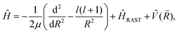 | (1) |
where
μ represents the reduced mass,
l(
l + 1) are the eigenvalues of the orbital angular momentum squared operator
![[l with combining circumflex]](https://www.rsc.org/images/entities/i_char_006c_0302.gif) 2
2,
![[V with combining circumflex]](https://www.rsc.org/images/entities/i_char_0056_0302.gif)
(
![[R with combining right harpoon above (vector)]](https://www.rsc.org/images/entities/i_char_0052_20d1.gif)
) is the potential energy surface (PES), and
ĤRAST is the internal Hamiltonian of an asymmetric top molecule satisfying:
31–33| | | ĤRAST|jτm,s〉 = εsjτ|jτm,s〉, | (2) |
where
εsjτ denote the eigenenergies and
s = 0, 1 the parity of the RAST molecule. The total wave function at a given energy
E for a given value of the total angular momentum
J, its projection
M to the space-fixed
z-axis, and the total inversion parity
p is given by:
| | 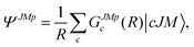 | (3) |
where the channel subscript
c brings together the four subscripts
j,
τ,
s,
l and |
cJM〉 = |
jτslJM〉 represent the channel wavefunctions (we will drop from now on the mentions to
J,
M and
p to simplify the notation). The latter wavefunctions are obtained by coupling the angular momentum of the RAST with the relative orbital angular momentum of the molecule as:
| | 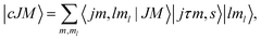 | (4) |
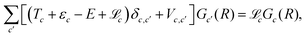
Using the expansion of the total wave function in the angular basis, the Schrödinger equation for the atom plus molecule system can be written as a set of coupled equations, usually known as the close-coupling equations:
| | 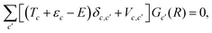 | (5) |
where
| |  | (6) |
and with
Vc,c′ representing the matrix elements of the potential,
| | | Vc,c′ = 〈c||c′〉. | (7) |
Restricting the semi-infinite radial domain of definition of this equation,
R ∈ [0, +∞[, to the finite inner region (0 <
R <
a) makes the Hamiltonian operator non-Hermitian. Adding a Bloch operator,
20| | 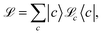 | (8) |
enables to recover the Hermiticity:
| |  | (9) |
| | 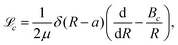 | (10) |
where
Bc is a real and energy-independent boundary parameter, which is usually assumed to be zero for scattering calculations.
To solve eqn (9), the radial wave function in the internal region is expanded in a basis set of N Lagrange mesh functions23φi(R) as:
| | 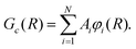 | (11) |
By using this expansion and defining a C matrix such as:
| | Cci;c′j(E,Bc) = 〈φi|(Tc + εc − E + ![[script L]](https://www.rsc.org/images/entities/char_e144.gif) c)δc,c′ + Vc,c′(R)|φj〉, c)δc,c′ + Vc,c′(R)|φj〉, | (12) |
and after carefully following the methodological development of Bocchetta and Gerratt
25 we obtain the expression for the R-matrix at the boundary as:
| | 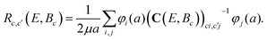 | (13) |
Another definition of the R-matrix can be given by considering the eigenvalues
En and the corresponding normalised eigenvectors
υn of the matrix
C(0,
Bc):
and
υTnυn′= δn,n′. Using the eigenvalues and the eigenvectors of the matrix
C(0,
Bc) we can construct the spectral decomposition of the inverse of
C(
E,
Bc) as:
| | 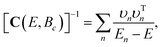 | (15) |
and the R-matrix becomes:
| | 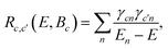 | (16) |
where the
| |  | (17) |
are the reduced widths or surface amplitudes which can be also represented as follows:
| |  | (18) |
where the prime indicates that the integration is carried out over all variables except
R.
2.2 H2O + H PES
The 4D PES used in this work is the one developed by some of the authors and used to study the rotational and vibrational bending relaxation of H2O colliding with H34 (P22 PES). A new 6D PES was also developed very recently for this system35 (P24 PES), whose accuracy was reported to be similar to that of the P22 PES. In order to compare R-matrix results with the published CC results obtained using the P22 PES, we perform our R-matrix calculations using the P22 PES. This allows us to overcome differences arising from the use of different PES.
3 Calculations
Following the R-matrix approach, we have conducted a study of the relaxation of all the excited rotational states of the water molecule within the j = 1, 2 and 3 multiplets, leading to 14 initial rotational states. Our basis set contains all the rotational states corresponding to 0 ≤ j ≤ 9. Calculations were carried out separately for the para (p) and ortho (o) symmetries of the water molecule, each involving a basis set of 50 rotational states.
The inner region equations were solved in the [3, 30]a0 radial interval for 31 values of the total angular momentum (0 ≤ J ≤ 30), a given total parity of the system (p = 0, 1) and a given p/o symmetry, leading to 124 matrices that needed to be stored. N × N Hamiltonian matrices are diagonalised with N ranging from minimum of N = 4000 to a maximum of N = 67![[thin space (1/6-em)]](https://www.rsc.org/images/entities/char_2009.gif) 000. A new code called RQMOLS was developed to solve the inner-part eigenvalue problem and store the eigenenergies and surface amplitudes in external files. By specifying different input options the code is also able to read the stored external files and apply the boundary condition to extract the scattering matrix S at the boundary of the inner region. As RQMOLS is interfaced with the Newmat code36,37 the S matrix can also be calculated inside the Newmat code at the boundary of the inner region or after propagation of the R-matrix. Indeed, the Newmat code36,37 is a scattering code that allows solving the CC equations in the space-fixed frame as outlined in the work of Green38 using a log-derivative propagator.18 The radial solutions are propagated up to asymptotic region where the asymptotic boundary conditions are applied to extract the scattering matrix.
000. A new code called RQMOLS was developed to solve the inner-part eigenvalue problem and store the eigenenergies and surface amplitudes in external files. By specifying different input options the code is also able to read the stored external files and apply the boundary condition to extract the scattering matrix S at the boundary of the inner region. As RQMOLS is interfaced with the Newmat code36,37 the S matrix can also be calculated inside the Newmat code at the boundary of the inner region or after propagation of the R-matrix. Indeed, the Newmat code36,37 is a scattering code that allows solving the CC equations in the space-fixed frame as outlined in the work of Green38 using a log-derivative propagator.18 The radial solutions are propagated up to asymptotic region where the asymptotic boundary conditions are applied to extract the scattering matrix.
4 Results and discussion
4.1 Bound states
We tested three different radial basis sets to solve the Schrödinger–Bloch equation (SBE) in the internal region. They are associated with a Lagrange–Legendre mesh shifted in the [0, 1] interval regularised by R denoted LG in Table 1 (eqn (3.128) and (3.129) ref. 39), and two Lagrange–Jacobi meshes shifted in the [0, 1] interval regularised by R (eqn (3.178) and (3.179) ref. 39) with a = 0, b = 3 denoted JC1 and a = 0, b = 30 denoted JC2. The results obtained for the low-lying bound states of the system are compared with the eigenvalues of the Schrödinger equation obtained with a 200-point Chebyshev DVR (CH)32,37,40 in Table 1. The computed eigenenergies of the Schrödinger and Schrödinger–Bloch equations are seen to be in excellent agreement. The different Lagrange meshes also produce practically the same results. For this reason, we opted for the Lagrange–Legendre mesh for all the calculations.
Table 1 Low lying bound states of the H–H2O system. CH denotes the eigenvalues of the Schrödinger equation obtained using a Chebyshev DVR grid. LG, JC1 and JC2 denote respectively the eigenvalues of the Schrödinger–Bloch equation obtained using a shifted Lagrange–Legendre mesh regularised by R, a shifted Lagrange–Jacobi mesh regularised by R with β = 3 and a shifted Lagrange–Jacobi mesh regularised by R with β = 30
| Assignment |
Radial basis |
J = 0 |
J = 1 |
J = 2 |
| H–pH2O |
| Σ(000)e |
CH |
−12.677 |
−10.372 |
−5.914 |
| LG |
−12.676 |
−10.371 |
−5.910 |
| JC1 |
−12.676 |
−10.371 |
−5.910 |
| JC2 |
−12.676 |
−10.371 |
−5.910 |
| Π(111)e |
CH |
|
24.189 |
26.479 |
| LG |
|
24.249 |
26.295 |
| JC1 |
|
24.249 |
26.295 |
| JC2 |
|
24.249 |
26.295 |
| Π(111)f |
CH |
|
27.031 |
31.471 |
| LG |
|
27.032 |
31.476 |
| JC1 |
|
27.032 |
31.476 |
| JC2 |
|
27.032 |
31.476 |
| H–oH2O |
| Σ(101)e |
CH |
12.622 |
11.066 |
13.311 |
| LG |
12.623 |
11.067 |
13.313 |
| JC1 |
12.623 |
11.067 |
13.313 |
| JC2 |
12.623 |
11.067 |
13.313 |
| Π(110)e |
CH |
|
17.540 |
23.780 |
| LG |
|
17.544 |
23.814 |
| JC1 |
|
17.544 |
23.814 |
| JC2 |
|
17.544 |
23.814 |
| Π(110)f |
CH |
|
13.814 |
18.251 |
| LG |
|
13.815 |
18.257 |
| JC1 |
|
13.814 |
18.257 |
| JC2 |
|
27.815 |
18.257 |
While for the present bound state calculations, the Bc = 0 choice ensures an excellent agreement between the Schrödinger and Schrödinger–Bloch eigenvalues, it is worth mentioning that it may not be the case for very specific problems. This point was discussed, for example by Baye et al.,23 where to ensure a good agreement between the calculated and analytically known bound state energies, Bc needed to be optimised in an iterative fashion. In the next paragraph which is dedicated to inelastic scattering calculations, since the choice of Bc = 0 has been proposed as the optimal one in the literature, this is the choice that we will use.
4.2 Rotationally inelastic cross sections
Cross sections for relaxation from all excited rotational states belonging to the j = 1, 2 and 3 multiplets of the water molecule have been computed for comparison with previous CC results.34 The angular basis set34 (eqn (2.1)) used to perform both the R-matrix and the CC calculations are identical while all the remaining parameters of the CC calculations can be found in this previous work.34 These multiplets correspond to 7 para and 7 ortho states. In our previous study, the CC calculations used a log-derivative propagator over the [3–30]a0 interval with a constant step size of 0.1a0. The current R-matrix calculations are then performed in the same internal region from [3–30]a0 and use a 200-point LG basis. The boundary conditions are applied directly at R = a = 30a0 without any further propagation being performed. We include partial waves up to Jmax = 30 ensuring a relative convergence of the cross sections better than 10−3.
The results obtained for the ortho 110,221,303 and para 111,220,313 initial states of H2O are presented in Fig. 1. The R-matrix and CC calculations show a high level of agreement, with the two types of curve being almost indistinguishable regardless of the initial state considered. The only minor discrepancies observed in the most pronounced resonant peaks can be attributed to the use of different energy grids. This level of accuracy is to be expected given that the R-matrix method is formally exact and the same approximations are used for both types of calculation.
 |
| | Fig. 1 State-to-state cross sections for the rotational relaxation of H2O by collision with H from several para/ortho initial states. Solid lines represent the CC cross sections and dotted lines the R-matrix cross-sections. Solid and dotted lines are fully overlapping, except for fine resonances structures. | |
This comparison also shows that applying the asymptotic boundary conditions at the boundary of the inner region produces accurate results, eliminating the need for further propagation. This assertion is indeed applicable to the system under consideration in this study, namely a collision between neutral particles with only one of the partners being polar, which involves an interaction potential that decays more rapidly than  . This would not be true for systems involving stronger long-range potentials, such as collisions between two neutral dipolar molecules or two ions, or between one ion and a neutral partner. This remark however does not apply to the ultra cold regime where the asymptotic matching radius is so large that direct diagonalization over the entire interval becomes computationally impractical.
To illustrate this point, we will consider the simple example of an elastic collision between an ion and an atom, namely the Na+ + He system. The potential energy curve (PEC) used here is the same than the one used in a previous study.41 In this one-dimensional scenario, increasing the number of grid points within the internal region does not present any computational challenges. Nevertheless, to demonstrate the role of R-matrix propagation, we present in Fig. 2 three different scenarios: (i) R-matrix calculations without propagation over the interval [0.2, 50]a0; (ii) calculations restricted to the shorter interval [0.2, 30]a0 without propagation; and (iii) calculations over [0.2, 30]a0 supplemented by propagation from 30 to 50a0 using the BBM R-matrix propagator.16 As can be seen, the calculation restricted to the shorter interval only converges for collision energies above 100 cm−1 and fails to reproduce the cross section at lower energies. By contrast, performing a short propagation over the interval [30, 50]a0 restores convergence with respect to the asymptotic matching radius, producing results from cases (i) and (iii) that are practically indistinguishable.
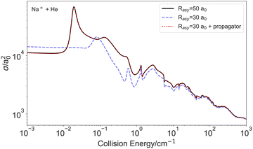 |
| | Fig. 2 Elastic cross section for the Na+ + He collision. Black solid lines represent the results obtained using the R-matrix method in a [0.2, 50]a0 interval, dashed blue lines represent the R-matrix calculations restricted to the shorter interval [0.2, 30]a0 without propagation while dotted red lines represent calculations over [0.2, 30]a0 supplemented by propagation from 30 to 50a0. The red dotted and black solid lines are fully overlapping. | |
4.2.1 Computational performance.
We conducted a test comparing the total computer time required by the two methods. The first step of the R-matrix approach which involves the construction and the diagonalization of 124 matrices needs 240 h and 24 min on 32 cores of the Intel Cascade Lake 6248 processor, with computation time for the para or ortho species being almost the same. The maximum memory allocated during the diagonalization stage was approximately 36 GB, corresponding to the storage and processing of the largest 67000 × 67000 double-precision matrix. Given that the computations were carried out independently for p-H2O and o-H2O, the comparison between the R-matrix and the CC computation times will be conducted solely for collisions involving one of the two species, the p-H2O. We then compare in Fig. 3 the R-matrix and CC computation times as a function of the number of collision energies for which the cross sections are calculated. The computation time presented is the one required to achieve the partial waves convergence of the cross section for five initial states independently of the size of the rotational basis set of p-H2O, which is constant.
 |
| | Fig. 3 Comparison of the R-matrix (in blue) and CC (in red) computation time. We consider three grids of respectively 100, 250, and 500 energies in the [0.1, 1000] cm−1 interval. The computation time required is specified over each bar. | |
As illustrated in this figure, for the smaller energy grid studied (100 energy points), the CC performs better than the R-matrix. This is due to the large time required in the diagonalization in the case of the R-matrix. Indeed the time required in the R-matrix calculation for this energy grid correspond to 121 hours, of which 120.20 hours correspond to the diagonalizations. For the two other energy grids studied, R-matrix dominates the comparison, with times significantly smaller than the respective CC times. This can be explained by realizing that in the R-matrix calculations, if we exclude the diagonalization time, which is independent of the number of energy, the time required for each grid is 0.80, 3.05, and 8.45 hours respectively. This time is practically negligible with respect to the total time required by the diagonalizations, making the scale in time of the R-matrix very efficient.
When considering the convergence of multiple initial states and large grids of collision energies, the computational advantage of the R-matrix is becoming more and more important. Significant computational gains can therefore be expected when dealing with the inelastic dynamics problems that are currently of interest in the fields of astrochemistry and atmospheric chemistry. The computational advantage of the R-matrix over CC calculations simply comes from the fact that, for the last method, a large amount of computer time is used to calculate the potential matrix values at each point on the radial grid. In the case of two neutral fragments interacting, we have seen that the asymptotic boundary conditions can be applied at the boundary of the inner region of the R-matrix method, with no further propagation required. This is a pivotal point that will increase the advantage of the R-matrix method when considering molecules with a greater number of internal degrees of freedom, as this adds complexity to the calculation of the matrix elements of the potential.
Further improvements in the R-matrix computation times can be achieved by reducing the cost of the diagonalization step, which—as discussed previously—represents the most computationally demanding part of the R-matrix workflow. To address this limitation, we explored the use of GPUs to accelerate the diagonalization process. Specifically, we performed the same diagonalization using the MAGMA GPU library,22 employing the dsyevd_m routine on three H100 GPUs in the gpu_p6 partition of the Jean Zay supercomputer.42 With these hardware specifications, the total diagonalization time decreased from 120.20 hours (CPU execution) to 3.83 hours (GPU execution), resulting in a substantial acceleration of the computational workflow.
A comparison of the diagonalization times for six angular momentum intervals is presented in Fig. 4. For each interval, we have carried out 10 diagonalizations corresponding to the five values of the total angular momentum and the two total parities, except in the first interval where 12 diagonalizations have been carried out. As shown in the figure, the use of GPUs leads to a dramatic reduction in total computation time, highlighting the remarkable efficiency of GPU-accelerated diagonalization. This achievement opens promising perspectives for extending R-matrix calculations to larger molecular systems.
 |
| | Fig. 4 Comparison of the R-matrix time performance using CPU (in blue) and GPUs (in green) to carry out the diagonalizations. We have divided the diagonalizations in intervals of the total angular momentum J. For each interval we have solve the diagonalization of all the values included in the interval and the two total parities. | |
5. Conclusions
In this work, we presented a comprehensive application of the R-matrix method to inelastic collisions involving an atom and a RAST molecule, as exemplified by the collision between H and rigid H2O. This system was chosen because its medium size is representative of what is typically needed in astrochemistry. We performed R-matrix calculations of the inelastic relaxation cross section for all the excited rotational states belonging to the j = 1, 2 and 3 multiplets of the water molecule, and compared the results with the CC calculations presented in a previous study.34 The R-matrix calculations in the inner region were carried out using a newly developed code RQMOLS interfaced with a modified version of the NEWMAT36,37 CC code allowing both to propagate the R matrix and apply the boundary conditions to extract the S matrix. The agreement between the R-matrix and CC calculations is found to be remarkable, with the curves representing the R-matrix and CC state-to-state cross sections being almost indistinguishable. These results demonstrate the R-matrix method's excellent performance in treating complex inelastic molecular scattering problems. We further tested the two possibilities of extracting the S matrix directly from the R-matrix calculated at the boundary of the inner region or after propagation in the asymptotic region. In the present case of interaction between two neutral species, we find that the long-range potential is not strong enough to require propagation over long distances. In other words the S matrix can be extracted directly from the R-matrix at the boundary of the inner region, which makes the R-matrix calculations even faster. This would not be the case for systems involving stronger long-range potentials, such as collisions between two neutral dipolar molecules or two ions, or between one ion and a neutral partner which would require further propagation as illustrated in the paragraph dedicated to the Na+ + He collision. We eventually compared the computation times required for the R-matrix and CC calculations and found that the former provides a clear performance advantage. As shown before, for small energy grid, CC offers a better performance. However, the R-matrix method becomes more attractive for larger energy grids, becoming 1.3× faster for the 250 energy grid and up to 3.7× faster for the largest one, highlighting its superior scalability with increasing energy resolution. This advantage becomes even more pronounced when using GPUs, which enable the rapid diagonalization of large matrices. In particular, employing the MAGMA library on the H100 GPUs partition reduces the diagonalization time from 120.20 hours (CPU) to 3.83 hours (GPU), a remarkable 31-fold speedup that significantly enhances the overall computational efficiency of the R-matrix approach.
In conclusion, the present results establish that the R-matrix method is a viable and efficient alternative to the CC formalism for modelling inelastic collisions between atoms and molecules. Its scalability, considered in conjunction with the potential for leveraging contemporary high-performance computing architectures, suggests a broad applicability to more complex systems where CC calculations are currently impractical. Subsequent research will concentrate on extending the methodology to encompass additional degrees of freedom and to address polyatomic systems of astrophysical and atmospheric relevance.
Conflicts of interest
There are no conflicts to declare.
Data availability
Data for this article, including data files and jupyter notebooks used to generate the Fig. 1 and 2 plots, are available at the Zenodo repository at https://doi.org/10.5281/zenodo.17909785.
Acknowledgements
This work was performed using HPC resources from GENCI-IDRIS (Grant 2025-AD010816507 (RMGV) and Grant 2025-AD010816183 (TS)). Support from the French Agence Nationale de la Recherche (ANR-Waterstars), Contract No. ANR-20-CE31-0011, and ANID/FONDECYT Exploración No. 13250044 projects is gratefully acknowledged. RMGV thanks Philippe Aurel for a helpful discussion regarding the software optimisation. We also acknowledge the use of the computing facility of Université de Bordeaux et Université de Pau et des Pays de l'Adour.
References
-
B. T. Draine, Physics of the Interstellar and Intergalactic Medium, Princeton University Press, Princeton, NJ, 2011 Search PubMed.
- S. Massalkhi, M. Agúndez, J. Cernicharo and L. Velilla-Prieto, Astron. Astrophys., 2020, 641, A57 CrossRef PubMed.
-
R. W. Schunk and A. F. Nagy, Ionospheres: Physics, Plasma Physics, and Chemistry, Cambridge University Press, Cambridge, UK, 2nd edn, 2009 Search PubMed.
-
M. Capitelli, C. M. Ferreira, B. F. Gordiets and A. I. Osipov, Plasma Kinetics in Atmospheric Gases, Springer, Berlin, Heidelberg, 2000, vol. 31 Search PubMed.
-
C. K. Law, Combustion Physics, Cambridge University Press, Cambridge, UK, 2006 Search PubMed.
- A. M. Arthurs and A. Dalgarno, Proc. R. Soc. London, Ser. A, 1960, 256, 540–551 Search PubMed.
- R. T. Pack, J. Chem. Phys., 1974, 60, 633–639 CrossRef.
- G. A. Parker and R. T. Pack, J. Chem. Phys., 1978, 68, 1585–1601 Search PubMed.
- D. Yang, X. Hu, D. H. Zhang and D. Xie, J. Chem. Phys., 2018, 148, 084101 CrossRef PubMed.
- E. P. Wigner, Phys. Rev., 1946, 70, 15 CrossRef.
- E. P. Wigner and L. Eisenbud, Phys. Rev., 1947, 72, 29 Search PubMed.
- P. G. Burke, A. Hibbert and W. D. Robb, J. Phys. B: At. Mol. Phys., 1971, 4, 153 CrossRef.
- J. Tennyson, Phys. Rep., 2010, 491, 29–76 CrossRef.
-
P. G. Burke, R-Matrix Theory of Atomic Collisions, Springer, Berlin, Heidelberg, 2011 Search PubMed.
- J. C. Light, R. B. Walker, E. B. Stechel and T. G. Schmalz, Comput. Phys. Commun., 1979, 17, 89–97 CrossRef.
- K. Baluja, P. Burke and L. Morgan, Comput. Phys. Commun., 1984, 35, C-823 CrossRef.
- B. R. Johnson, NRCC Proc., 1979, 5, 86 Search PubMed.
- D. E. Manolopoulos, J. Chem. Phys., 1986, 85, 6425–6429 Search PubMed.
-
D. E. Manolopoulos, PhD thesis, University of Cambridge, 1988.
- C. Bloch, Nucl. Phys., 1957, 4, 503–528 CrossRef.
-
A. Jhunjhunwala and G. Talavera, Accelerating GPU Applications with NVIDIA Math Libraries, NVIDIA Developer Blog, 2022, https://developer.nvidia.com/blog/accelerating-gpu-applications-with-nvidia-math-libraries/.
- S. Tomov, J. Dongarra and M. Baboulin, Parallel Comput., 2010, 36, 232–240 CrossRef.
- D. Baye, M. Hesse, J. M. Sparenberg and M. Vincke, J. Phys. B: At., Mol. Opt. Phys., 1998, 31, 3439–3454 CrossRef.
- P. Descouvemont and D. Baye, Rep. Prog. Phys., 2010, 73, 44 CrossRef.
- C. J. Bocchetta and J. Gerratt, J. Chem. Phys., 1985, 82, 1351–1362 CrossRef.
- C. J. Bocchetta, J. Gerratt and G. Guthrie, J. Chem. Phys., 1988, 88, 975–984 CrossRef.
- J. Tennyson, L. K. McKemmish and T. Rivlin, Faraday Discuss., 2016, 195, 31–48 RSC.
-
T. Rivlin, L. K. McKemmish and J. Tennyson, Quantum Collisions and Confinement of Atomic and Molecular Species, and Photons, Singapore, 2019, pp. 257–273 Search PubMed.
- T. Rivlin, L. K. McKemmish, K. E. Spinlove and J. Tennyson, Mol. Phys., 2019, 117, 3158–3170 CrossRef.
- L. K. McKemmish and J. Tennyson, Philos. Trans. R. Soc., A, 2019, 377, 20180409 CrossRef.
-
R. N. Zare, Angular Momentum, Wiley, New York, 1988 Search PubMed.
- R. M. García-Vázquez, O. Denis-Alpizar and T. Stoecklin, J. Phys. Chem. A, 2023, 127, 4838–4847 CrossRef PubMed.
- R. M. García-Vázquez, A. Bergeat, O. Denis-Alpizar, A. Faure, T. Stoecklin and S. B. Morales, Faraday Discuss., 2024, 251, 205–224 RSC.
- L. D. Cabrera-González, O. Denis-Alpizar, D. Páez-Hernández and T. Stoecklin, Mon. Not. R. Astron. Soc., 2022, 514, 4426–4432 CrossRef.
- B. Yang, C. Qu, J. M. Bowman, D. Yang, H. Guo, N. Balakrishnan, R. C. Forrey and P. C. Stancil, J. Phys. Chem. Lett., 2024, 15, 11312–11319 CrossRef PubMed.
- T. Stoecklin, O. Denis-Alpizar, A. Clergerie, P. Halvick, A. Faure and Y. Scribano, J. Phys. Chem. A, 2019, 123, 5704–5712 CrossRef PubMed.
- T. Stoecklin, L. D. Cabrera-González, O. Denis-Alpizar and D. Páez-Hernández, J. Chem. Phys., 2021, 154, 144307 CrossRef PubMed.
- S. Green, J. Chem. Phys., 1976, 64, 3463–3473 CrossRef.
- D. Baye, Phys. Rep., 2015, 565, 1–107 CrossRef.
- R. M. García-Vázquez, L. D. Cabrera-González, O. Denis-Alpizar and T. Stoecklin, ChemPhysChem, 2024, 25, e202300752 CrossRef PubMed.
- R. M. García-Vázquez, T. Stoecklin and P. Halvick, Phys. Rev. A, 2025, 112, 062812 CrossRef.
- IDRIS, CNRS, Jean Zay Supercomputer-GPU Partition Specifications, https://www.idris.fr/eng/jean-zay/cpu/jean-zay-cpu-hw-eng.html#gpu_p6, 2024, Accessed: 2025-10-20.
|
| This journal is © the Owner Societies 2026 |
Click here to see how this site uses Cookies. View our privacy policy here. 
 *a,
Lisan David
Cabrera-González
*a,
Lisan David
Cabrera-González


 . This would not be true for systems involving stronger long-range potentials, such as collisions between two neutral dipolar molecules or two ions, or between one ion and a neutral partner. This remark however does not apply to the ultra cold regime where the asymptotic matching radius is so large that direct diagonalization over the entire interval becomes computationally impractical.

