Quantitative analysis of FAI-diffusion in sequentially evaporated FAPbI3 perovskite thin films
Received
25th August 2025
, Accepted 20th March 2026
First published on 8th April 2026
Abstract
Physical vapor deposition of perovskite solar cells is gaining increasing importance due to its up-scaling potential applicability for the industrial manufacturing. Especially the layer-by-layer sequential approach allows for a more precise process and stoichiometry control and offers cross-contamination free deposition. However, a detailed analysis of perovskite film formation and growth is usually only done qualitatively, with a limited number of studies addressing this aspect. We want to start filling the gap of lacking quantitative evaluations by investigating the phase evolution inside the PbI2–FAI diffusion couple during deposition and annealing with an in situ X-ray diffraction (XRD) system. The observed diffraction intensity transients allow us to calculate the diffusion coefficient of the diffusing species for different isothermal annealing temperatures. With a derived Arrhenius plot, the activation energy and preexponential factor for the diffusion constant is determined. This report describes the mathematical model underlying the evaluation as well as application to a PbI2–FAI (FA+: formamidinium CH(NH2)2+) diffusion couple, i.e. two initially separated layers brought into contact, enabling interdiffusion and reactive perovskite formation upon annealing. We find a linear trend in the Arrhenius plot, resulting in an activation energy of 0.83 eV. A variation of the initial parameters shows only minor activation energy changes, indicating a robust underlying mathematical model.
1. Introduction
The first successful introduction of organo-metal-halide perovskite solar cells (PSCs) into the field of photovoltaics in 20091 came along with a huge rise of attention for this material class. In the following years many techniques to prepare the PSCs got invented with spin-coating yielding the, to date, highest power conversion efficiency (PCE) of 27.0%.2 However, this preparation method bears several disadvantages like the insufficient upscaling potential3,4, low material yield and the usage of environmental-toxic solvents.5,6
A solvent-free alternative are vacuum-based deposition techniques such as physical vapor deposition (PVD). In this field Snaith et al. are the pioneers with their co-evaporated MAPbI3−xClx (MA+: methylammonium CH3NH3+) solar cell (PCE of 15.4%).7 However, controlling the perovskite stoichiometry is challenging for co-evaporated absorbers due to inevitable fluctuations of material fluxes reaching the substrate. A more precise stoichiometry control can be achieved via sequential layer-by-layer deposition of each individual precursor.5,8 Additionally, sequential thermal evaporation of the organic ammonium salts and lead halides allows the deposition of both species in separated vacuum chambers, reducing cross-contamination.8,9 Using this technique Li et al. recently reached a PCE of 24.42% for Cs0.05FA0.95PbI38. For sequentially evaporated PSCs, material diffusion, which is driven by concentration gradients, is a key process. However, there are only few publications about sequentially evaporated PSC and only limited knowledge concerning the concentration-driven ionic diffusion kinetics during the annealing step exists.
In contrast to the concentration-driven diffusion, investigations of the ionic drift due to an external electric field already exist since 2015. At this time Tress et al.10 proposed the idea, that the J–V-hysteresis effect could originate from the existence of mobile ions within the MAPbI3 perovskite absorber. This assumption was theoretically verified by Haruyama et al.11 using density functional theory (DFT) calculations for MAPbI3 and FAPbI3. They also determined the activation energies for the ionic drift of I−, MA+, and FA+ ions to be 0.44–0.48 eV, 0.57 eV and 0.61 eV, respectively. An experimental verification was published by Eames et al.12 using chronophotoampereometry measurements. In their work the activation energies for I− and MA+ ion drift in MAPbI3 were calculated to be 0.58 eV and 0.84 eV, leading to comparable values to Haruyama et al. Also, the ionic drift activation energy of Pb2+ ions was determined as 2.31 eV, indicating a neglectable diffusion of the metal ion and a rather stable PbI2 framework. In 2019 Futscher et al.13 conducted a deeper analysis of ion migration in MAPbI3 perovskites using transient capacitance measurements. They were able to not just calculate the activation energies (0.29 eV for I− and 0.39–0.90 eV for MA+) but also the ion density and diffusion coefficient (at 300 K). For I− they calculated 3.1 × 10⁻⁹ cm2 s−1 and 1.6 × 10⁻¹²–6.8 × 10⁻¹² cm2 s−1 for MA+, respectively. Furthermore, the comparable slower MA+ ion diffusion was assigned to be the origin of the J–V-hysteresis effect, while the I− ions relax too fast to have a significant effect on the J–V curves.
As already mentioned, knowledge about activation energies and diffusion coefficients for concentration-driven diffusion is still underexplored. To fill this gap, we conducted systematic experiments to evaluate the kinetics of the diffusion-reaction mechanisms of sequentially evaporated PbI2 and FAI films and their diffusion/reaction kinetics during annealing. For that purpose, we prepared FAPbI3 films via sequential thermal evaporation of PbI2 and FAI and subsequently annealed the layer stack in the same vacuum chamber (see Fig. 1). The vacuum chamber is equipped with an in situ X-ray diffraction (XRD) set up that allows to monitor the evolution of the crystalline phases within the film in quasi real-time. After depositing PbI2 and FAI we subjected the layer stack to a series of different isothermal annealing conditions, while recording the X-ray diffraction patterns of the evolving film. By comparing the diffusion kinetics of layer stacks isothermally annealed at different temperatures, we were able to extract the kinetic parameters for this process and generate a holistic diffusion model approach, allowing us to determine the diffusion coefficient for different temperatures and from this the activation energy. For the verification of the model we also performed SEM measurements and determined the final film thickness and morphology. Finally, an error estimation of the calculated diffusion coefficients and activation energy is conducted.
 |
| | Fig. 1 Schematic illustration of the used PbI2–FAI diffusion couple, with the perovskite growing between them during the annealing. | |
2. Experimental section
2.1 Substrates
For all experiments, we used commercial glass substrates coated with ITO (100 nm) provided by KINTEC. The cleaning of the coated substrates was performed in three steps using an ultrasonic bath. In the first step we used a cleaning soup with water and 1% EMAG EM-080, followed by isopropyl alcohol (IPA) and acetone for 15 min each. After cleaning we spin-coated the hole transport layer (HTL) poly[bis(4-phenyl)(2,4,6-trimethylphenyl)amine] (PTAA). For that a solution of 2.5 mg ml−1 in toluene was used. The samples were then transferred to a glove box, which is directly attached to our vacuum chamber.
2.2 Perovskite formation
The source materials for evaporation, PbI2 (99.999%, Thermo Scientific) and FAI (>99.99%, Greatcell), were stored in the attached glove box and were used as received. These materials were sequentially deposited via thermal evaporation onto the glass-ITO-PTAA substrate. Firstly, PbI2 was evaporated (645 nm, 0.5–0.8 Å s−1, 6.16 g cm−3 (ref. 14)) and subsequently FAI (1200 nm, 1.0–2.0 Å s−1, 2.48 g cm−3 (ref. 15)). The deposited amount of each reactant was monitored by a quartz crystal microbalance (QCM) and by laser light scattering (LLS). During the deposition the substrate temperature was 25 °C. An example of the in situ XRD data obtained, as well as the explanation of the LLS technique, is given in Fig. S1 and the corresponding paragraph in the SI. It is important to note, that the temperature reading during the following annealing step is done on the back side of the sample, where the heating element is placed, leading to a discrepancy between nominal (back side) and real (front side) temperature. We performed experiments with self-adhesive temperature labels to estimate the real temperature on the front side, where the material stack is located. In Fig. S4 a photograph of these labels (front side temperature) is shown together with the nominal back side temperature. Based on this, we estimate the temperature difference in the chosen temperature range (90–120 °C) to be around 16 °C (see SI). This will be considered when the Arrhenius graph is plotted, but in the following, the experiments will still be labelled with respect to the nominal back side temperature. The sequential deposition results in a FAI/PbI2 double layer stack of around 2000 nm total thickness. The FAI film thickness was chosen about twice as thick as the PbI2 layer with a 2![[thin space (1/6-em)]](https://www.rsc.org/images/entities/char_2009.gif) :1 FAI:PbI2 particle ratio to guarantee a quasi-infinite FAI material source (see section “Derivation of Diffusion Model”). The vacuum chamber has a base pressure of 2 × 10⁻⁵ mbar and a maximum operational pressure of 1 × 10⁻⁴ mbar. Monitoring of the pressure was done with an Edwards WRGS-NW35 wide range gauge.
:1 FAI:PbI2 particle ratio to guarantee a quasi-infinite FAI material source (see section “Derivation of Diffusion Model”). The vacuum chamber has a base pressure of 2 × 10⁻⁵ mbar and a maximum operational pressure of 1 × 10⁻⁴ mbar. Monitoring of the pressure was done with an Edwards WRGS-NW35 wide range gauge.
2.3 XRD measurements
During evaporation and annealing, XRD in situ measurements were performed, where the entering/exiting X-rays passed through Kapton windows installed in the evaporation chamber walls. The Kapton windows were replaced after each process in order to reduce absorption of X-rays by deposited material. For the in situ XRD, Cu-Kα radiation (wavelength 1.54 Å) from an X-ray tube with a power of 1.6 kW (40 kV, 40 mA) was used. The Kβ radiation was attenuated via a Ni-filter to 5% of the Kα intensity. The setup is capable of measuring one XRD scan with an angular range of 28° every 120 s with a linear detector array consisting of three Dectris Mythen 1 K modules. Because of the three individual detector modules, two small detector gaps arise in the measured diffractograms. During in situ measurements, the setup uses a fixed source-detector ω (incident) and Ω (detector) geometry. In all experiments ω = 9° and Ω = 13° were used. Only diffraction peaks, which have the same incident and outgoing angle (θ–2θ condition) are in the focus point of the goniometer circle. All other diffraction peaks are out of focus and thus have a larger full width at half maximum (FWHM). The experiments were conducted at constant annealing temperatures. A more detailed description of the in situ XRD setup can be found in ref. 16–19. One scan was performed accumulating the diffraction intensity for the period of 120 s. Between the scans there is a downtime of 2 s for data transfer. This downtime is considered in the time stamp of the experiment. Fig. 2 shows exemplarily the in situ XRD data for the annealing process at 100 °C in a colormap representation. The remaining colormaps of the other annealing temperatures can be found in the SI. In Fig. 3, a qualitative comparison of the different diffusion/reaction kinetics for different isothermal annealing (initial heating takes 10 min) temperatures in the temperature range between 90 °C and 120 °C is shown for one characteristic FAPbI3 perovskite peak. With these experiments, we can show that: (i) a complete conversion from the FAI/PbI2 layer stack is possible (extinction of the FAI and PbI2 peaks). (ii) The time for the diffusion/reaction and perovskite formation to be completed decreases from about roughly 200 min (at 90 °C annealing) to roughly 50 min (at 120 °C annealing). The integrated peak intensities were fitted with the program PDXL version 2.8.1.1 by Rikagu Inc. using a split pseudo-Voigt line profile. The evolution of the diffraction patterns provides us with a time-resolved information of the different crystal phases involved, and in the integrated intensities of their characteristic peaks lies the information of how much of this phase is present (basically the film thickness in a one-dimensional diffusion model). To minimise the influence of different preferred orientations, a weighted sum over all detectable PVK reflections was applied. This procedure and the analysis of the XRD intensities is explained in more detail later on.
 |
| | Fig. 2 The top graph shows a color plot representing the normalized color coded diffraction intensity as a function of diffraction angle (y-axis) and time (x-axis). Example of annealing an PbI2/FAI stack at 100 °C. The middle graph shows the integrated intensities in counts per second of the 111 peak at 25.1° of orthorhombic FAI (red) and the 210 peak at 31.4° of cubic FAPbI3 (black). The bottom graph displays the evolution of the substrate temperature. | |
 |
| | Fig. 3
In situ diffractograms of the 3D 31.4° peak for all nominal temperatures. The red line indicates the adjusted tend. A gradually decreasing necessary annealing time is needed with increasing annealing temperature. | |
2.4 Film characterisation
To determine the final film thickness after each experiment SEM cross-section measurements were performed with a Zeiss Supra 40 VP. A secondary electron in-lens detector and an acceleration voltage of 5 kV was used. The SEM device is also equipped with a Bruker EDX detector. EDX measurement were performed using an acceleration voltage of 15 kV, a working distance of 6 mm and a magnification of 500. For quantification L-lines of iodine and M-lines of lead were used. Background correction and quantitative analysis were performed using a standardless method based on the ratio of peak intensity to background signal, combined with atomic number, absorption, and fluorescence correction ((P/B) ZAF fitting).
3. Derivation of diffusion model
In this section, the diffusion model we use to determine the diffusion coefficient D based on the in situ XRD data is explained. The standard approach for determination of diffusion coefficients is to measure concentration depth profiles with methods like glow discharge optical emission spectroscopy (GDOES)20 or secondary ion mass spectroscopy (SIMS).21 Both methods rely on sputtering through the sample. The GDOES technique has two major downsides. On the one hand, a reliable surface analysis is not achievable due to the initial building up of the plasma. On the other hand, controlling the shape of the sputter crater is difficult resulting in an increasing error with sputtering time. The major downside of SIMS is the so-called “matrix effect”. This effect leads to a different amount of ejected particles based on the underlying layers, making quantifications rather complex. As an alternative, we used in situ XRD to analyse the diffusion-reaction kinetics of the sequentially deposited perovskite layer stacks. XRD probes the bulk, and in this work, we consider integrated XRD peak intensities (peak areas) as proportional to the amount of a crystalline phase in the sample. Applying a diffusion model and fitting procedure to the time-dependent data of the in situ XRD measurements for a set of different isothermal annealing temperatures T allows us to extract the temperature dependent diffusion coefficient D(T) = D0 × exp(−Ea/(kBT)), where D0 is the preexponential factor, Ea the activation energy, and kB the Boltzmann constant. The following section will describe the experiment and derive a model to determine these diffusion coefficients and explain the technical and physical uncertainty sources like the intensity dependence from the ω (incident) and Ω (detector) angles, attenuation effects, and the coexistence of multiple perovskite phases, namely lower and higher dimensional perovskites (LDP and HDP).
3.1 Description of experiments and XRD analysis
To investigate perovskite formation, we sequentially deposited the reactants PbI2 and FAI on glass/ITO/PTAA substrates at room temperature in the first step (deposition). This process step was identical for all experiments, and the in situ XRD data representation of all depositions is presented as colormaps is in the SI, verifying the reproducibility of this process step (see Fig. S1 and S2).
In a following isothermal annealing step, the different species interdiffuse and a perovskite phase is formed. Fig. 2 shows exemplarily the in situ diffractogram of the annealing step for an experiment with a nominal isothermal annealing temperature of 100 °C (upper part). In these colormaps, the abscissa shows time, the ordinate the diffraction angle ω + Ω and the XRD intensity is color coded. In other words, in this data representation, each column corresponds to one XRD scan with an accumulation time of 120 s. For all experiments an angle of incidence of ω = 12° was chosen, bringing the ω + Ω region around 24° in the parafocus. Hence, all evaluated peaks are not too far from that focus condition and the resulting peak broadening is minimized. The 2 black regions in the colormaps stem from the before mentioned spatial gaps between the 3 detector modules. In the in situ diffractograms no Kβ signals are shown. The used Ni filter reduces the Kβ intensity to approximately 5% of the corresponding Kα signal. To correct for this residual Kβ contribution, 5% of the Kα intensity was subtracted from the measured intensity at each angle. The bremsstrahlung background is not subtracted. The middle graph shows the evolution of the integrated intensities of two characteristic Bragg reflexes, namely of the (111) peak of orthorhombic FAI (red) at 25.1° (ref. 15) and the (210) peak of cubic FAPbI3 (black) at 31.4°.22 Fig. S6 in the SI gives the same plot, but with labelling all detectable peaks. Please note, that with the chosen detector setting, no PbI2 peaks are detected, even during/after the deposition process, as is detailed in the SI. The bottom graph shows the substrate temperature. It is seen, that after around 10 min the desired nominal temperature of 100 °C is reached. In the upcoming sections the integrated intensities of several perovskite and FAI peaks are used to determine the diffusion coefficients. For that, Fick's second law is used to simulate the particle flux J, which is necessary for simulating the integrated XRD intensities. By comparing these intensities with the measured data, we calculate the diffusion coefficient for each isothermal experiment. In order to form the diffusion system, first a PbI2 layer and afterwards a FAI layer was deposited onto a glass/ITO/PTAA substrate. At the interface between the reactants PbI2 and FAI the perovskite is forming, and therefore the diffusion system to be considered is PbI2/Perovskite/FAI.
3.2 Assumptions and preconditions
Depending on their diffusion constants, both reactants PbI2 and FAI in principle can each diffuse through the perovskite towards the other reactant layer. However, a well-known fact from literature as well as from our own studies18,23 is that in this specific stack mainly the FAI is diffusing while PbI2 is not diffusing or only to a minor degree. This forms the first assumption or precondition of the following evaluation. Interestingly, it was found, that without voltage bias the FAI is diffusing as a complete molecule and not in dissociated form. For dissociative FA+ and I− diffusion, the presence of humidity is required.23 A second assumption of the upcoming evaluation is that the diffusion only occurs in one dimension, perpendicular to the substrate plane. In Fig. S8, a SEM cross-section of a PbI2–FAI film directly after deposition and before annealing is shown. Here, a clear interface with little interface roughness between both reactants is seen. This supports our assumption of a one-dimensional diffusion system. Thirdly, semi-infinite FAI and PbI2 layers are assumed to ensure constant boundary conditions (see Mathematical ansatz chapter). This means that our model is only valid until one of the reactant layers is completely consumed.
A fourth assumption for the model is that FAI species instantaneously react to perovskites as soon as FAI arrives at the PbI2|perovskite interface and encounters free PbI2 species. This assumption excludes the existence of FAI species within the PbI2 layer. Further, it encompasses that in the specific stack PbI2|FAI the perovskite growth is diffusion-controlled and not reaction controlled. The instantaneous reaction of FAI particles makes the PbI2 layer a sink for FAI, but with a moving boundary. Both reactants are consumed during the reaction and the perovskite thickness is increasing.
Another important point is that not only the ordinary cubic 3D perovskite FAPbI3 is formed during the annealing step, but also lower dimensional perovskites (LDP), for example the 2D perovskite FA2PbI4 (2D) or perovskites with even lower dimensions. A more detailed analysis of all existing phases during our experiments will be given in Section 4. In this evaluation, we do not differentiate between different diffusion coefficients in the different PVK phases but rather derive an effective value over all phases. In the following we will refer to the product layer consisting of all possible perovskite dimensionalities as the “perovskite” or “PVK” layer.
Furthermore, we assume a concentration independent diffusion coefficient, making it a constant value within the perovskite layer, independently of the dimensionality.
Next, an assumption regarding the depth-dependent concentration profile of the diffusing FAI particles is necessary. A schematic representation of the concentration profiles at different times is shown in Fig. 4. As already described above, within the PbI2 layer no FAI can exist due to the “instantaneous” formation of FAI and PbI2 to FAPbI3 at the beginning of the diffusion process (which here actually starts to some extent already at room temperature during the deposition of FAI) only FAI and PbI2 are present. We can define the concentration of FAI (particles per volume) within the FAI-layer as c0. This value is calculated via the unit cell volume of FAI (461.06 Å3) and the number of FAI particles (formula unit Z) within this volume (4 particles)15 to 14.36 mmol cm−3. As soon as some perovskite has formed (independent of the dimensionality) a certain FAI concentration gradient will form inside the perovskite layer. From the FAI side, FAI molecules will diffuse into the perovskite. At the perovskite|PbI2 interface, FAI molecules will diffuse out of the perovskite and form new perovskite. Therefore, at the FAI|PVK interface the FAI concentration will be highest, and then gradually decrease within the perovskite towards the PVK|PbI2 interface. Here, two boundary conditions are of importance: there is a maximum amount of FAI (molar concentration) that can exist within the perovskite film, the saturation concentration cs. It is important to recall, that “perovskite” includes not just the ordinary 3D FAPbI3, but also all LDPs. At the FAI|PVK interface the concentration of FAI will amount to this value. In the following, we present two approaches on how to derive this saturation concentration cs.
 |
| | Fig. 4 Schematic concentration profiles for t = 0 (left), t = t0 (middle), and t > t0 (right). Inside the FAI and PbI2 reactants, the FAI concentrations are constant at c0 and 0, respectively. Within the perovskite a monotonuos decrease is assumed with cs being the left and cm being the right boundary condition at the interfaces. | |
For the experimental determination of cs, we conducted a simple experiment where FAI is deposited on a heated substrate with an already deposited PbI2 layer. The increased substrate temperature prevents FAI accumulation on top of the PbI2 layer due to immediate interdiffusion and PVK formation. The FAI deposition continues until the first traces of a separate, crystalline FAI phase is detectable in the XRD. This marks the time, when no more FAI can be built into the PVK structure and FAI crystallizes as a second phase. Following EDX measurements allow to calculate the FAI:PbI2 ratio for the moment that the first FAI peaks occurred. In Fig. 5 the experiment is shown. 60 nm of PbI2 were evaporated on ITO/PTAA (ITO peak positions: 21.5, 30.6, and 35.4° (ref. 24)), afterwards the nominal substrate temperature was increased to 100 °C, then FAI was evaporated on the heated PbI2 film. Due to the higher substrate temperature, the sticking coefficient of FAI on the substrate reduces. This leads to a smaller deposition rate, but larger FAI diffusivity. After 100 min, the PbI2 peak at 12.7° starts to decrease and the FAPbI3 (100) and (200) peaks at 14° and 28° respectively start to increase. Upon further FAI deposition and diffusion, the 3D FAPbI3 (100) and (200) peaks decrease again and a 3D (111) & LDP peaks at 24° start to appear. A clear distinction between the 3D (111) peak at 24.22°, the 2D (110) peak at 24.27°, and the 1D (104) peak at 24.07° is not possible due to their close proximity. This intensity change from mainly 14° and 28° to 24° signalises the transition from the ordinary 3D phase to LDP phases. We closed the FAI shutter after 200 min for 20 min to verify, that no FAI is piling up on the surface. As seen, the integrated intensities do not change during that time, suggesting the absence of a FAI layer, which would still keep diffusing into the layer in that time. After 220 min., the FAI shutter was reopened. After 250 min, a monoclinic FAI (![[1 with combining macron]](https://www.rsc.org/images/entities/char_0031_0304.gif) 02) peak at 28° starts to appear. This means, that at t = 250 min the saturation concentration of FAI in a PVK layer is reached. After closing the shutter a second time, the integrated intensities do not change again, indicating that no further FAI can be dissolved inside the PVK structure. The following EDX measurements result in an approximate FAI:PbI2 ratio of 4:1 extrapolated to the time t = 250 min. We calculated the tooling factor for the deposition of FAI on the heated substrate to calculate back via QCM how much FAI was deposited until 250 min. The FAI:PbI2 ratio of 4:1 is consistent with the ratio of a the 0D FA4PbI6 perovskite, which is the PVK phase with the lowest dimension (highest FAI content), so these results are consistent. Due to the lack of literature on that specific phase we cannot calculate the saturation concentration (as FAI particles per volume) for this 0D FA4PbI6 phase. To nevertheless estimate the saturation concentration, we can compare the FA-based system with the chemical similar MA-system. Here, Yokoyama et al. calculated the crystal structure for all dimensionalities, from 3D MAPbI3 up to 0D MA4PbI6.25 When calculating the saturation concentration of MAI in all these lattices (see Table S1), a monotonous increasing trend with decreasing dimensionality can be seen. This is also valid for the normalised saturation concentration cs/c0 (c0,MAI = 14.08 mmol cm−3). In the FA-system, the normalised concentration (c0,FAI = 14.36 mmol cm−3) for the 3D and 2D is similar to the MA-system. Because no structural information is known in the literature for the 1D FA3PbI5 and 0D FA4PbI6, we assume a similar trend of increased normalised concentration cs/c0. Following this route of thoughts, we assume a FAI normalised saturation concentration of cs/c0 of 80% as an upper limit, as in the MA-system.
02) peak at 28° starts to appear. This means, that at t = 250 min the saturation concentration of FAI in a PVK layer is reached. After closing the shutter a second time, the integrated intensities do not change again, indicating that no further FAI can be dissolved inside the PVK structure. The following EDX measurements result in an approximate FAI:PbI2 ratio of 4:1 extrapolated to the time t = 250 min. We calculated the tooling factor for the deposition of FAI on the heated substrate to calculate back via QCM how much FAI was deposited until 250 min. The FAI:PbI2 ratio of 4:1 is consistent with the ratio of a the 0D FA4PbI6 perovskite, which is the PVK phase with the lowest dimension (highest FAI content), so these results are consistent. Due to the lack of literature on that specific phase we cannot calculate the saturation concentration (as FAI particles per volume) for this 0D FA4PbI6 phase. To nevertheless estimate the saturation concentration, we can compare the FA-based system with the chemical similar MA-system. Here, Yokoyama et al. calculated the crystal structure for all dimensionalities, from 3D MAPbI3 up to 0D MA4PbI6.25 When calculating the saturation concentration of MAI in all these lattices (see Table S1), a monotonous increasing trend with decreasing dimensionality can be seen. This is also valid for the normalised saturation concentration cs/c0 (c0,MAI = 14.08 mmol cm−3). In the FA-system, the normalised concentration (c0,FAI = 14.36 mmol cm−3) for the 3D and 2D is similar to the MA-system. Because no structural information is known in the literature for the 1D FA3PbI5 and 0D FA4PbI6, we assume a similar trend of increased normalised concentration cs/c0. Following this route of thoughts, we assume a FAI normalised saturation concentration of cs/c0 of 80% as an upper limit, as in the MA-system.
 |
| | Fig. 5
In situ diffractograms of the saturation concentration determination experiment represented as a colormap. After depositing PbI2, the substrate was heated to a nominal temperature of 100 °C and FAI got deposited. Up to 250 min, all FAI is incorporated into the PVK structure. After this time, a crystalline FAI secondary phase is forming. The peaks at 21.5°, 30.6°, and 35.4° are from the substrate (ITO). | |
For an alternative derivation of a lower limit for cs, we can consider the 2D FA2PbI4, which we clearly detect in the in situ XRD, as the PVK phase with highest FAI content that we clearly detect in the XRD. As can be seen in Table S1 of the SI, the 2D FA2PbI4 phase has a relative saturation concentration cs of 70%. With the hypothesis that this 2D phase will form at the FAI|PVK interface, the normalised saturation concentration then would read 70%. This leads to a normalised saturation concentration range of 70–80%. In the “Discussion” chapter the influence of the selected saturation concentration will be assessed.
The second important interface in the diffusion system is PVK|PbI2. This interface defines the minimum concentration of FAI cm, that is needed to grow a PVK. In literature as well as in our own studies18,26, no PbI2 rich phases for the FA-system exist. This results in 3D FAPbI3 being the perovskite with the lowest FAI content. The calculated concentration of that phase (6.46 mmol cm−3, 45%) marks the minimum concentration. Both, cs and cm, are important boundary conditions for our model.
3.3 Mathematical ansatz
After discussing the physical assumptions, the mathematical derivation is described. In a first step a numerical solution for the depth dependent concentration c of FAI within the PVK phase will be presented. In a second step the correlation between the measured XRD intensities and the concentration gradient will be discussed.
We start with Fick's second diffusion law
| |  | (1) |
Here
c describes the concentration of FAI within the PVK layer.
D is the diffusion coefficient of FAI in the PVK layer, which here is assumed to be constant throughout the PVK layer and is not changing with time.
t and
z are the time and the one-dimensional space coordinate, respectively. The coordinate system is chosen in the relative system of the PVK layer, such that the FAI|PVK interface is fixed to
z = 0 and the PVK|PbI
2 interface is at
z =
dPVK (see
Fig. 4), although for an external observer both interfaces are moving in opposite directions. We are thus looking for a solution to
eqn (1) in the domain 0 ≤
z ≤
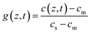
dPVK. To solve the partial differential equation (PDE) we need the following starting and boundary conditions, which derive from the assumptions in Section 3.2:
| | | c(z = dPVK(t), t > t0) = cm | (4) |
Fick's law
(1) together with the conditions
(2)–(4) is a so called initial-boundary problem. More precise, it is an initial-boundary problem with inhomogeneous moving boundaries, since the position of the right boundary of the PVK layer depends on the (time dependent) perovskite thickness
dPVK(
t). The mathematical solution of such a moving boundary problem is not trivial and it is more convenient to transform it into an initial-boundary problem with homogeneous, fixed boundaries first. To this end, we first define a function
for which we obtain
| |  | (5) |
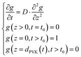
Now, the right boundary is homogeneous, but still moving in time. To fix it, we define a new function
f(
z′,
t) =
g(
z′
dPVK(
t),
t), which realizes a scaling of the position axes. Problem
(5) then becomes:
| |  | (6) |
Here, the term
d′
PVK(
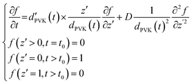
t) describes the time derivative of the PVK layer thickness. Now we finally arrived at a system with fixed, homogeneous boundaries and standard numeric methods like finite differences can be applied. The original function
c(
z,
t) can then be obtained from
f(
z′,
t) by
| |  | (7) |
Eqn (6) shows, that the PDE requires the knowledge of the perovskite thickness time evolution. The thickness increase of the PVK layer, however, depends on the amount of FAI which arrives at the right PVK|PbI
2 interface.
dPVK(
t) must therefore be determined self-consistently with
eqn (6). To this end, we first examine the thickness increase Δ
dPVK within a small time step Δ
t and we can write
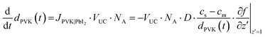
| | | ΔdPVK = JPVK|PbI2·VUC·NA·Δt | (8) |
Here,
VUC and
NA describe the unit cell volume and Avogadro's constant, respectively. The FAI particle flux
JPVK|PbI2 is calculated
via Fick's first law, which by virtue of
eqn (7) can be written as
| |  | (9) |
Plugging
eqn (9) into
eqn (8) and performing a transition to infinitesimal time steps, leads to:
| |  | (10) |
This is a first order ordinary differential equation, whose solution can be computed to
| |  | (11) |
| |  | (12) |
The equation system
(6) now has to be solved by taking
eqn (12) into account. To this end, we chose an iterative approach. For the first iteration a constant perovskite thickness equivalent to the starting thickness is used:
d0PVK(
t) =
dPVK,0. This is plugged into
eqn (6) and a 0th approximation
f0(
z′,
t) to
f(
z′,
t) is calculated by a finite difference method. This is then used, to calculate an updates thickness
d1PVK(
t)
viaeqn (12). This procedure is repeated until sufficient convergence is reached. At the end of this first step, we have a self-consistent solution
dPVK(
t) and, by
eqn (7),
c(
z,
t).
After knowing the concentration profile, the link to the measured XRD intensities can be derived. Therefore, the correlation between concentration c(t) and the absolute number of FAI particles NPVK|PbI2, which diffuse through the PVK|PbI2 interfaces in the time interval between t0 and t, needs to be written. This is done by integration of the FAI particle flux J through the PVK|PbI2 interface over time.
| |  | (13) |
By utilizing
eqn (13), the final equation for the simulated integrated PVK XRD intensity is:
| |  | (14) |
Here, we assume a direct proportionality between the measured integrated XRD intensity
I and the number of FAI particles
N, that diffuse through each interface. The proportionality factor
λPVK is defined by the molar mass
M and mass density
ϱ of the perovskite (4.09 g cm
−3),
22 as well as the ratio between intensity and film thickness

. A more detailed discussion of this proportionality can be found in the SI. As the annealing starts with a small amount of PVK already present at the beginning of the experiment, a starting intensity
I0 has to be considered.
Eqn (14) allows to fit the increase of the perovskite peak intensities during the annealing experiment. To simulate the FAI peak decrease, an analogous derivation can be performed by considering the FAI|PVK interface for the concentration gradient. This results in the following formulas:
| |  | (15) |
| |  | (16) |
| |  | (17) |
Our algorithm, which is based on the finite difference approach, is simulating a theoretical integrated intensity transient for a given set of
cs,
cm, and
D and comparing it to the measured data
via calculating the deviation
Ω as
| |  | (18) |
With these equations the diffusion coefficients, which represent the data best, can be calculated. In the following section this will be shown exemplary on one diffusion experiment while for the other temperatures, we only give the extracted diffusion coefficients.
4. Results
This section will show exemplarily for the isothermal experiment at nominal 100 °C how a single isothermal annealing experiment is evaluated. The substrate reaches a nominal temperature of 100 °C after 10 min. During this heating phase the diffraction peaks at 24.7°, 25.6°, and 31.0° decrease drastically in intensity and new peaks arise at 25.1° and 32.8°. This indicates the transformation of FAI from the monoclinic to the orthorhombic phase.15,27 The orthorhombic FAI peaks then decrease in intensity during the annealing experiment due to diffusion of FAI through the FAI|PVK interface to the PVK|PbI2 interface, where they form new perovskite. As soon as an FAI particle crosses the FAI|PVK interface, it does not contribute to the FAI peak intensity anymore (see eqn (17)). The intensity decrease of the 25.1° (FAI 111) peak is shown in red in Fig. 2. Furthermore, a large number of peaks from PVK phases of all dimensionalities evolve during the annealing. These can be attributed to the 3D and 2D. For the 1D FA3PbI5 no literature data and thus no reference peak positions exist. However, a known phase is the 1D (CI(NH2)2)3PbI5 with an iodoformamidinium (CI(NH2)2+ = iFA+) cation instead of a formamidinium (CH(NH2)2+ = FA+) cation. The diffraction peaks attributed to that phase fit with our experimental data. We therefore assign this 1D (iFA)3PbI5 phase as one of our products in the perovskite layer, through which the FAI is diffusing.28 The diffraction peaks, which are detectable in our experiments are: 13.8° (1D), 13.9° (3D), 19.7° (3D), 24.1° (1D), 24.2° (3D), 27.8° (1D), 28.0° (3D), 29.1° (1D), 30.0° (1D) and 31.4° (3D). Additionally, a 2D peak is located at 25.6°, which is in superposition with the orthorhombic FAI (111) peak, leading to a large fitting uncertainty. Because of that, this peak is not taken into consideration for the diffusion coefficient determination. Fig. S6 shows all mentioned peaks in the in situ diffractogram. Fig. S7 shows a diffractogram of the FAI and 2D PVK (03) peak. All these PVK peaks are increasing in intensity during the annealing, indicating the formation of new PVK material. Since in the presented approach the XRD peak intensity is used for the quantification of the share of a certain phase, one has to exclude the influences of texture and grain reorientation. To this end, the weighted peak sum of all detectable PVK peaks was evaluated instead of single PVK peaks. For that, the peaks have been normalised according to the following formula:29,30| |  | (19) |
with Irel being the normalisation factor:| |  | (20) |
All constants and peak-independent parameters like initial intensity I0 or detector sensitivity are combined in the scaling factor SCF. Also, the structure amplitude |F|2, the multiplicity MU, geometric correction  , and polarisation term P = 1 + cos2(ω + Ω) impact the resulting relative intensity. Here, ω and Ω describe the angle of incident and detector angle for the X-rays, respectively. Table S2 gives the values for all factors in eqn (20) for every used PVK peak.
In addition, we performed an experiment, where we co-evaporated FAPbI3 and measured the integrated intensity of the PVK 24° peak (sum of 1D and 3D) in dependency of the deposited PVK thickness. In Fig. S10 it can be seen by the almost linear behaviour of the intensity vs thickness that for a film thickness below 2 µm, attenuation effects are neglectable. This verifies the direct proportionality  as stated in the previous section.
Fig. 6 shows the I(t) graphs for each normalised PVK peak as well as the weighted sum of all of them (black). Here we like to emphasize, that not every peak area evolution has the same shape. While the 3D peaks (dotted) mainly have a larger intensity increase at the beginning of the experiment, the 1D peaks (dashed) rise more towards the end of the annealing phase. For the weighted sum (black) a monotonous increasing integrated intensity is seen. Additionally, selected error bars from peak fitting are shown for the 1D PVK peak at 24° to demonstrate, that uncertainties arising from the fitting procedure are minor. For the following fitting procedure, only the weighted integrated intensity sum IPVK will be used for the diffusion product. Additionally, the orthorhombic (111) FAI peak is evaluated as the reactant phase. For the fitting, a starting time t0 of 10 min was chosen, after which the desired temperature (here nominal 100 °C) is reached. Additionally, within these 10 min the phase transition from monoclinic to orthorhombic FAI occurs, which explains the jump in the IFAI data. In order to fulfil the assumption of a semi-infinite FAI source, the end time for the fitting is set to the time where the simulated FAI intensity falls to 10% of the initial intensity, which is after 87.4 min (tend). The saturation concentration cs and minimum concentration cm are 11.49 mmol cm−3 and 6.46 mmol cm−3 respectively. Also needed are the initial (dPVK,0) and the final (dSEM) PVK thicknesses. During the deposition period of the experiment some PVK already has formed, leading to a non-zero starting thickness for the evaluation (see Fig. S1). We have taken the 3D-PVK peak at 31.4° as a measurement to estimate the initial thickness. For that we used the maximum integrated intensity (316 cps°) and α from that 31.4° peak at the end of the annealing experiment (1.44 cps° per nm) to calculate dPVK,0 to be 219 nm. The influence of the starting thickness is discussed later. The final PVK thickness was determined via SEM (see Fig. S9) to around 1850 nm. In Table S3 all initial parameters for all experiments are listed. Fig. 7 shows the calculation results. In the upper graph the measured (dotted) data are shown for the PVK (blue) and FAI (red). The solid lines represent the fits with the optimised diffusion coefficient D = 4.66 × 10⁻¹² cm2 s−1. The lower graph shows the simulated perovskite growth according to eqn (12) as a solid line. Here, the dotted line represents an extrapolation, as if the condition of unlimited FAI and PbI2 supply would be guaranteed. It can be seen, that the final measured SEM PVK thickness (1850 nm) and the extrapolated PVK thickness (1930 nm) are in good agreement, supporting the reliability of our calculated diffusion coefficient. This resulting diffusion coefficient was used for the Arrhenius plot.
 |
| | Fig. 6 Normalised integrated intensities of all visible PVK peaks as well as the weighted sum of all of them. All graphs are individually normalised. Dashed line represents all 3D peaks, dotted 1D, and full line shows the weighted sum. For the 1D peak at 24° some error bars are shown. | |
 |
| | Fig. 7 Normalised measured data as well as simulated intensities for the FAI (111) peak and the weighted sum of all detectable PVK signals (top) and time dependent thickness of the PVK layer (bottom). tend is set to 87.4 min. The resulting diffusion coefficient is D = 4.66 × 10⁻¹² cm2 s−1. | |
The evaluation has been performed for all experiments from 90 °C to 120 °C in 5 °C steps. The Arrhenius plot in Fig. 8 shows the diffusion coefficients of all isothermal annealing experiments as a function of inverse temperature. Note, that the real substrate temperature is estimated 16 K below the nominal temperature, due to the temperature difference between front and back side of the sample (following the calibration procedure detailed in the SI). It can be seen, that all points are following the linear trend. The resulting activation energy is 0.84 eV and the preexponential factor 3.63 cm2 s−1. The error bars were acquired by calculating the Gaussian error propagation. For the Gaussian error propagation, the individual uncertainties were determined from the maximum deviation of the evaluated parameters cs, dPVK,0, and t0, which will be discussed in the next chapter. This results in an uncertainty of the activation energy of ±0.18 eV. Due to the logarithmic scale, the error for the preexponential factor Δln(D0) is asymmetric. The uncertainty interval is D0 ∈ [1.20 × 10⁻²; 1.10 × 10+3] cm2 s−1. Fig. 3 shows the in situ diffractograms of the 3D PVK peak at 31.4° for all nominal temperatures, together with the adjusted tend. As expected, the needed time to complete the diffusion decreases with higher annealing temperature. Similar to Fig. 7, the fit results of the remaining temperatures are shown in Fig. S13.
 |
| | Fig. 8 Arrhenius plot with error bars of all seven experiments with cs/c0 = 80%. The calculated activation energy is Ea = 0.84 eV and the preexponential factor is D0 = 3.63 cm2 s−1. The temperature data are corrected to the calibrated values as described in the text. | |
5. Discussion
In the following, we will check how strongly the chosen boundary and starting conditions of our fitting procedure impact on the results, in order to estimate the error of our findings. Then, a comparison with literature values will be given.
5.1 Effect of saturation concentration cs
Firstly, we will check how strongly the choice of the saturation concentration (70–80%) impacts on the results. For this, we conducted the same calculation with a normalised saturation concentration of 70%, 75% and 80%. The results are shown in Fig. 9. An increase in cs/c0 leads to lower diffusion coefficients in the chosen temperature interval. The correlation between saturation concentration and diffusion coefficient is shown in Fig. 10. A fit-error-minimum band is seen, indicating that the cs and D cannot be fitted simultaneously. Because of that, cs was estimated with an additional experiment and set to 80%, as discussed in Section 3.2. By varying the normalised saturation concentration between 70 and 80%, the activation energy changes by 0.02 eV (2.4%). Additionally, D0 differs within the same order of magnitude due to the difference in Ea (slope). Variations in the saturation concentration only weakly affect the concentration gradient at the PVK|PbI2 interface and therefore have a negligible influence on the FAI flux for sufficiently thick perovskite layers, leaving the extracted diffusion coefficients and thus Arrhenius parameters almost unchanged.
 |
| | Fig. 9 Arrhenius plot for cs/c0 of 70%, 75% and 80% to estimate uncertainty due to saturation concentration variation. | |
 |
| | Fig. 10 Relative fit error Ω in dependency of the diffusion coefficient D and the normalised saturation concentration, with a constant minimum concentration cm. No global minimum is seen, but a “minimum-band”. This implies a correlation between cs and D. | |
5.2 Effect of different PVK starting thickness dPVK,0
To analyse the effect of a different starting PVK thickness dPVK,0, the same evaluations were done with a starting thickness of 100 and 500 nm. The saturation concentration was set to cs/c0 = 80%. The Arrhenius plots are shown in Fig. S10. Choosing a smaller dPVK,0 results in no change in the activation energy and preexponential factor. Upon increasing the starting thickness to 500 nm, Ea and D0 increase by 0.05 eV and 8.82 cm2 s−1, respectivly. While a smaller initial perovskite thickness increases the early-time FAI flux, the growth rate decreases at longer annealing times following the characteristic  behaviour, such that variations in the starting thickness do not significantly affect the diffusion coefficient obtained from long-time kinetics.
5.3 Effect of different starting times t0
Also, a variation of the starting time t0 was performed. For that, besides the used 10 min, also 8 and 12 min were tested, which means starting the fitting procedure one measurement point earlier or later, respectively. The results can be seen in Fig. S12. A minor decrease in activation energy (0.04 eV) can be seen between 10 and 12 min, whereas Ea increases by 0.07 eV between 10 and 8 min. This also decreases (increases) the preexponential factor by a factor of 4 (10) between 10 and 12 min (8 min). Shifting the effective start time results in a horizontal displacement of the diffusion-controlled PVK growth curve but has only a minor impact on the final perovskite thickness at long annealing times, where the growth rate is low.
5.4 Comparison with literature and contextualisation
The activation energy of 0.84 eV as determined by our experiments is comparable to values found at the chemically similar MA-based system. Eames et al. calculated the activation energy to 0.58 eV and 0.84 eV for I− and MA+, respectively, using their chronophotoampereometry measurement.12 Futscher et al. published 0.29 eV for I− and 0.39–0.90 eV for MA+via capacitance measurements.13 It can be seen, that our value for Ea is close to the reported MA+ activation energies.
In the SI we calculated the diffusion coefficient at 105 °C from Arrhenius parameters for selected publications.12,13,31 Table S4 shows, that different measurements techniques result in diffusion coefficient discrepancies of multiple orders of magnitude (10−14–10−9 cm2 s−1). Our value of 7.07 × 10⁻¹² cm2 s−1 is located within that interval, verifying the comparability of both chemical similar organic A-cations.
First principle calculation report migration barriers for halides and A-cations in the range of 0.44–0.48 eV (I−), 0.57 eV (MA+), and 0.61 eV (FA+).11 The small difference between MA+ and FA+ highlights the chemical similarity of the organic A-site cations. Additionally, Ghasemi et al. performed experiments to extract diffusion parameters for bulk and grain boundary diffusion. They reported lower activation energies for GB diffusion (0.46–0.57 eV) compared to bulk diffusion (0.61–0.74 eV).32 Also, a recently published work by Siegert et al. utilizes in situ XRD measurements to determine activation energies for the diffusion of I− into MAPbBr3 (0.32 eV) and Br− into MAPbI3 (0.59 eV). Their model makes use of the Boltzmann–Matano approach combined with Rietveld refinement of the perovskite diffraction peaks.33 A similar model was used by Wollstadt et al. to obtain diffusion parameters in oxide perovskites utilizing in situ XRD.34 Overall, the activation energies obtained in our work are slightly higher than most previous reported values. This difference can be rationalized by the distinct experimental configuration and diffusion geometry employed here, which differs from commonly investigated systems.
Our comparatively high preexponential factor D0 arises from defect-mediated transport and the high defect densities characteristic of halide perovskites35 and therefore represents effective transport prefactors rather than bulk diffusion parameters.36 Futscher et al. give values for the diffusion coefficient at 300 K, which translates (together with the Ea values) to values for D0 in the range of 10−6 to 103 cm2 s−1 for the MA+ ions. Ghasemi et al. determined preexponential factors on the order of 10−3 cm2 s−1 for bulk and 10−1 cm2 s−1 for grain boundary diffusion and are thus within the same range as values from this work.32
For future solar cell device upscaling approaches, a low annealing time is desired. For example, for a τ = 1 min annealing step, the necessary annealing temperature can be estimated with our results. Preparing a L = 2 µm thick absorber and utilizing  , a diffusion coefficient of D = 6.67 × 10⁻¹⁰ cm2 s−1 is necessary. Performing an extrapolation using the Arrhenius parameters, a temperature of 168 °C can be calculated. Considering the low annealing time, no significant degradation effects should apply to the film.
6. Summary
We conducted experiments to quantify the FAI diffusion through the PVK layer in the diffusion system PbI2–PVK–FAI. For this purpose, we deposited via sequential deposition a stack of pure PbI2 + FAI layers via sequential deposition. A following isothermal annealing step allowed us to determine the diffusion coefficient for the chosen annealing temperature by a mathematical model, utilising the in situ XRD system. Comparing data from experiments conducted at different annealing temperatures allows to make an Arrhenius plot and determined the preexponential factor D0 and activation energy Ea to 1.20 × 10⁻²–1.10 × 10+3 cm2 s−1 and 0.84 ± 0.18 eV, respectively. This work leads the way to advanced insight into the diffusion and perovskite growth for sequential deposition and annealing processes. Our goal for the future is to analyse more material systems and quantify the effect by adding different ions into the FAPbI3 system. For example, caesium and chloride are said to increase the diffusivity and thus perovskite growth.8,37
Author contributions
T. S., R. S., and P. P. developed the experimental procedure. T. S. and M. M. mathematically described the used diffusion model. The base code was created by M. S. and T. S. expanded it. P. P. guided the scientific progress. T. S. deposited the films and evaluated the experiments. T. S., M. M., R. S., and P. P. discussed and interpreted the results. T. S. wrote the main manuscript.
Conflicts of interest
There are no conflicts to declare.
Data availability
Data for this article, including the XRD and experimental deposition/annealing data are available at https://cloud.uni-halle.de/s/0fmJ80Aag8T42Dt.
Supplementary information (SI) containing XRD colormaps, fit plots and fit parameters. See DOI: https://doi.org/10.1039/d5cp03252k.
Acknowledgements
The German Research Foundation (DFG) under contract number SCHE-1745/9-1 and the Spanish Ministry of Science, Innovation and Universities under contract number (CNS2024-154809) provided gratefully acknowledged financial support. M. M. acknowledges funding by BMWK/PTJ (Project PVKIS) under contract number (03EE1206D). Funding for open access publishing: Universidad Pablo de Olavide/CBUA.
References
- A. Kojima, K. Teshima, Y. Shirai and T. Miyasaka, Organometal Halide Perovskites as Visible-Light Sensitizers for Photovoltaic Cells, J. Am. Chem. Soc., 2009, 131(17), 6050–6051 CrossRef CAS PubMed.
- Best Research-Cell Efficiency Chart|Photovoltaic Research|NREL, [cited 2025 June 27]. Available from: https://www.nrel.gov/pv/cell-efficiency.
- J. H. Lee, B. S. Kim, J. Park, J. W. Lee and K. Kim, Opportunities and Challenges for Perovskite Solar Cells Based on Vacuum Thermal Evaporation, Adv. Mater. Technol., 2023, 8(20), 2200928 CrossRef CAS.
- S. R. Bae, D. Y. Heo and S. Y. Kim, Recent progress of perovskite devices fabricated using thermal evaporation method: perspective and outlook, Mater. Today Adv., 2022, 14, 100232 Search PubMed.
- J. Feng, Y. Jiao, H. Wang, X. Zhu, Y. Sun and M. Du,
et al., High-throughput large-area vacuum deposition for high-performance formamidine-based perovskite solar cells, Energy Environ. Sci., 2021, 14(5), 3035–3043 Search PubMed.
- R. Vidal, J. A. Alberola-Borràs, S. N. Habisreutinger, J. L. Gimeno-Molina, D. T. Moore and T. H. Schloemer,
et al., Assessing health and environmental impacts of solvents for producing perovskite solar cells, Nat. Sustain., 2020, 4(3), 277–285 CrossRef.
- M. Liu, M. B. Johnston and H. J. Snaith, Efficient planar heterojunction perovskite solar cells by vapour deposition, Nature, 2013, 501(7467), 395–398 CrossRef CAS PubMed.
- H. Li, J. Zhou, L. Tan, M. Li, C. Jiang and S. Wang,
et al., Sequential vacuum-evaporated perovskite solar cells with more than 24% efficiency, Sci. Adv., 2022, 8(28), eabo7422 CrossRef PubMed.
- Y. Vaynzof, The Future of Perovskite Photovoltaics—Thermal Evaporation or Solution Processing?, Adv. Energy Mater., 2020, 10(48), 2003073 CrossRef CAS.
- W. Tress, N. Marinova, T. Moehl, S. M. Zakeeruddin, M. K. Nazeeruddin and M. Grätzel, Understanding the rate-dependent J–V hysteresis, slow time component, and aging in CH3NH3PbI3 perovskite solar cells: the role of a compensated electric field, Energy Environ. Sci., 2015, 8(3), 995–1004 RSC.
- J. Haruyama, K. Sodeyama, L. Han and Y. Tateyama, First-Principles Study of Ion Diffusion in Perovskite Solar Cell Sensitizers, J. Am. Chem. Soc., 2015, 137(32), 10048–10051 CrossRef CAS PubMed.
- C. Eames, J. M. Frost, P. R. F. Barnes, B. C. O’Regan, A. Walsh and M. S. Islam, Ionic transport in hybrid lead iodide perovskite solar cells, Nat. Commun., 2015, 6(1), 7497 CrossRef CAS PubMed.
- M. H. Futscher, J. M. Lee, L. McGovern, L. A. Muscarella, T. Wang and M. I. Haider,
et al., Quantification of ion migration in CH3NH3PbI3 perovskite solar cells by transient capacitance measurements, Mater. Horiz., 2019, 6(7), 1497–1503 RSC.
-
W. M. Haynes, CRC Handbook of Chemistry and Physics, CRC Press, 97th edn, 2017 Search PubMed.
- A. A. Petrov, E. A. Goodilin, A. B. Tarasov, V. A. Lazarenko, P. V. Dorovatovskii and V. N. Khrustalev, Formamidinium iodide: crystal structure and phase transitions, Acta Crystallogr., Sect. E: Crystallogr. Commun., 2017, 73(Pt 4), 569–572 Search PubMed.
- T. Burwig and P. Pistor, Reaction kinetics of the thermal decomposition of MAPbI3 thin films, Phys. Rev. Mater., 2021, 5(6), 065405 CrossRef CAS.
- P. Pistor, T. Burwig, C. Brzuska, B. Weber and W. Fränzel, Thermal stability and miscibility of co-evaporated methyl ammonium lead halide (MAPbX3, X = I, Br, Cl) thin films analysed by in situ X-ray diffraction, J. Mater. Chem. A, 2018, 6(24), 11496–11506 Search PubMed.
- K. L. Heinze, T. Schulz, R. Scheer and P. Pistor, Structural Evolution of Sequentially Evaporated (Cs,FA)Pb(I,Br)3 Perovskite Thin Films via In Situ X-Ray Diffraction, Phys. Status Solidi A, 2024, 221(3), 2300690 CrossRef CAS.
- S. Hartnauer, L. A. Wägele, F. Syrowatka, G. Kaune and R. Scheer, Co-evaporation process study of Cu2ZnSnSe4 thin films by in situ light scattering and in situ X-ray diffraction, Phys. Status Solidi A, 2015, 212(2), 356–363 CrossRef CAS.
- D. Zheng, P. Volovitch and T. Pauporté, What Can Glow Discharge Optical Emission Spectroscopy (GD-OES) Technique Tell Us about Perovskite Solar Cells?, Small Methods, 2022, 6(11), 2200633 CrossRef CAS PubMed.
- S. P. Harvey, Z. Li, J. A. Christians, K. Zhu, J. M. Luther and J. J. Berry, Probing Perovskite Inhomogeneity beyond the Surface: TOF-SIMS Analysis of Halide Perovskite Photovoltaic Devices, ACS Appl. Mater. Interfaces, 2018, 10(34), 28541–28552 CrossRef CAS PubMed.
- D. H. Fabini, C. C. Stoumpos, G. Laurita, A. Kaltzoglou, A. G. Kontos and P. Falaras,
et al., Reentrant Structural and Optical Properties and Large Positive Thermal Expansion in Perovskite Formamidinium Lead Iodide, Angew. Chem., Int. Ed., 2016, 55(49), 15392–15396 Search PubMed.
- D. Lin, J. Fang, X. Yang, X. Wang, S. Li and D. Wang,
et al., Modulating the Distribution of Formamidinium Iodide by Ultrahigh Humidity Treatment Strategy for High-Quality Sequential Vapor Deposited Perovskite, Small, 2023, 2307960 Search PubMed.
- N. Nadaud, N. Lequeux, M. Nanot, J. Jové and T. Roisnel, Structural Studies of Tin-Doped Indium Oxide (ITO) and In4Sn3O12, J. Solid State Chem., 1998, 135(1), 140–148 CrossRef CAS.
- T. Yokoyama, S. Ohuchi, E. Igaki, T. Matsui, Y. Kaneko and T. Sasagawa, An Efficient ab Initio Scheme for Discovering Organic–Inorganic Hybrid Materials by Using Genetic Algorithms, J. Phys. Chem. Lett., 2021, 12(8), 2023–2028 Search PubMed.
- K. L. Heinze, P. Wessel, M. Mauer, R. Scheer and P. Pistor, Stoichiometry dependent phase evolution of co-evaporated formamidinium and cesium lead halide thin films, Mater. Adv., 2022, 3(23), 8695–8704 RSC.
- M. Bukleski, S. Dimitrovska-Lazova and S. Aleksovska, Vibrational spectra of methylammonium iodide and formamidinium iodide in a wide temperature range, Maced. J. Chem. Chem. Eng., 2019, 38(2), 237–252 Search PubMed.
- S. Wang, D. B. Mitzi, C. A. Feild and A. Guloy, Synthesis and Characterization of [NH2C(I):NH2]3MI5 (M = Sn, Pb): Stereochemical Activity in Divalent Tin and Lead Halides Containing Single.ltbbrac.110.rtbbrac. Perovskite Sheets, J. Am. Chem. Soc., 1995, 117(19), 5297–5302 Search PubMed.
-
B. D. Cullity, Elements Of X Ray Diffraction, Addison-Wesley Publishing Company, Inc., 1956, p. 531, Available from: https://archive.org/details/elementsofxraydi030864mbp Search PubMed.
-
M. Birkholz and P. F. Fewster, High-Resolution X-ray Diffraction, Thin Film Analysis by X-Ray Scattering, John Wiley & Sons, Ltd, 2005, pp. 297–341. Available from: https://onlinelibrary.wiley.com/doi/abs/10.1002/3527607595.ch7 Search PubMed.
- A. Senocrate, I. Moudrakovski, G. Y. Kim, T. Y. Yang, G. Gregori and M. Grätzel,
et al., The Nature of Ion Conduction in Methylammonium Lead Iodide: A Multimethod Approach, Angew. Chem., 2017, 129(27), 7863–7867 CrossRef.
- M. Ghasemi, B. Guo, K. Darabi, T. Wang, K. Wang and C. W. Huang,
et al., A multiscale ion diffusion framework sheds light on the diffusion–stability–hysteresis nexus in metal halide perovskites, Nat. Mater., 2023, 22(3), 329–337 Search PubMed.
- T. Siegert, P. Pahwa, M. Griesbach, F. J. Kahle, H. Oberhofer and A. Köhler,
et al., Modelling Thermal Halide Exchange of Perovskite Powders With and Without BMIMBF4 From an Interdiffusion Perspective, Adv. Funct. Mater., 2025, e10920 Search PubMed.
- S. Wollstadt, R. A. De Souza and O. Clemens, Kinetic Study of the Interdiffusion of Fluorine and Oxygen in the Perovskite-Type Barium Ferrate System BaFeO2.5−xF2x, J. Phys. Chem. C, 2021, 125(4), 2287–2298 CrossRef CAS.
- A. Walsh, D. O. Scanlon, S. Chen, X. G. Gong and S. H. Wei, Self-Regulation Mechanism for Charged Point Defects in Hybrid Halide Perovskites, Angew. Chem., Int. Ed., 2015, 54(6), 1791–1794 CrossRef CAS PubMed.
-
P. Shewmon, Diffusion in Solids, in Diffusion in Solids, ed. P. Shewmon, Springer International Publishing, Cham, 2016 DOI:10.1007/978-3-319-48206-4_1.
- J. Yan, J. Nespoli, R. K. Boekhoff, H. Wang, T. Gort and M. Tijssen,
et al., Chloride-improved crystallization in sequentially vacuum-deposited perovskites for p–i–n perovskite solar cells, Sustainable Energy Fuels, 2025, 9(10), 2729–2737 RSC.
|
| This journal is © the Owner Societies 2026 |
Click here to see how this site uses Cookies. View our privacy policy here. 
 Open Access Article
 This Open Access Article is licensed under a Creative Commons Attribution-Non Commercial 3.0 Unported Licence
 a,
Matthias
Maiberg
a,
Matthias
Maiberg


 for which we obtain


 . A more detailed discussion of this proportionality can be found in the SI. As the annealing starts with a small amount of PVK already present at the beginning of the experiment, a starting intensity I0 has to be considered.


 , and polarisation term P = 1 + cos2(ω + Ω) impact the resulting relative intensity. Here, ω and Ω describe the angle of incident and detector angle for the X-rays, respectively. Table S2 gives the values for all factors in eqn (20) for every used PVK peak.
 as stated in the previous section.


 behaviour, such that variations in the starting thickness do not significantly affect the diffusion coefficient obtained from long-time kinetics.
 , a diffusion coefficient of D = 6.67 × 10⁻¹⁰ cm2 s−1 is necessary. Performing an extrapolation using the Arrhenius parameters, a temperature of 168 °C can be calculated. Considering the low annealing time, no significant degradation effects should apply to the film.