DOI:
10.1039/D5AY01528F
(Paper)
Anal. Methods, 2026,
18, 98-108
A lightweight two-dimensional convolutional neural network for soil nutrient prediction by visible–near-infrared spectroscopy
Received
12th September 2025
, Accepted 10th November 2025
First published on 1st December 2025
Abstract
Rapid and accurate estimation of soil nutrient content is essential for assessing soil fertility, facilitating sustainable nutrient management, and optimizing crop productivity. However, the high dimensionality of spectral data and the limitations of one-dimensional prediction models hinder prediction accuracy and efficiency. We propose a lightweight two-dimensional convolutional neural network, 2D-CTM-CNN, which integrates data compression and reconstruction to solve these problems. The framework transforms one-dimensional visible–near-infrared (VNIR) spectra into a two-dimensional representation and employs a Shapley-weighted 2D-CNN to predict nitrogen (N) and soil organic carbon (SOC). Comparative experiments against partial least squares regression (PLSR), a 1D-CNN, and two state-of-the-art 2D-CNN approaches (2D-GASF-CNN and 2D-MTF-CNN) demonstrate that 2D-CTM-CNN achieves superior performance, with relative prediction deviation (RPD) values exceeding 4 for both N and SOC. Relative to the 1D-CNN, R2 improved by 5.68% for N and 5.56% for SOC, while spectral dimensionality was reduced from 4200 to 54, substantially enhancing computational efficiency. These findings highlight the effectiveness of 2D-CTM-CNN for high-precision soil nutrient prediction, offering a scalable and efficient solution for advancing precision agriculture.
1 Introduction
Soil nutrients are the foundation of soil productivity and play a critical role in sustainable agricultural development. Soil organic carbon (SOC) enhances soil fertility by facilitating nutrient cycling, promoting water infiltration, and improving water retention, whereas nitrogen (N) is essential for key biochemical and physiological processes that directly affect crop productivity.1–3 However, conventional methods for measuring SOC and N are time-consuming, costly, environmentally detrimental, and inadequate for rapid assessment.4 These problems emphasize the urgent need for rapid, accurate, and cost-effective alternatives to predict soil nutrient content.
Visible–near-infrared (VNIR) spectroscopy has emerged as a widely accepted alternative owing to its simplicity, non-destructiveness, speed, and environmental friendliness.5,6 VNIR spectra, covering the 400–2500 nm range, capture distinct reflectance and absorption characteristics that form the basis for quantitative soil nutrient estimation. Nevertheless, the wide spectral range introduces challenges such as high dimensionality, spectral overlap, multicollinearity, and non-linear relationships with soil nutrients.7,8 Traditional modeling approaches, though effective to some degree, struggle to achieve robust and generalized predictions under such complexity. Moreover, linear dimensionality reduction techniques such as PCA often eliminate critical non-linear information, thereby limiting the performance of subsequent models.9
Deep learning (DL) provides superior computational efficiency and representation capability, particularly through hierarchical feature extraction that can capture complex non-linear patterns in spectral data.9 Among DL methods, convolutional neural networks (CNNs) are widely used and have demonstrated strong potential in agricultural applications. Veres et al. first applied CNNs to soil spectral data, confirming their feasibility for soil property evaluation10. Padarian et al. showed that multitask CNNs improved prediction accuracy for large-scale datasets,11 while Rashid et al. reported that CNN outperformed other architectures such as LSTM in predicting soil cadmium content.12 Despite the strong performance of 1D-CNNs, their limited structural representation restricts their ability to capture complex spectral patterns. In contrast, 2D-CNNs excel in image recognition tasks due to their ability to effectively model two-dimensional spatial structures.13,14 Converting one-dimensional spectra into two-dimensional representations is therefore considered a promising approach for improving feature expressiveness and prediction accuracy.
Recent studies have explored various 1D-to-2D spectral transformation methods to enhance soil property prediction. Yue et al. employed the Gramian Angular Field (GAF) to convert spectral data into 2D images, enabling CNNs to capture geo-spectral features more effectively.15 Wang et al. utilized Markov Transition Field (MTF) encoding with 2D-CNNs to predict aflatoxin B1 content in maize, achieving superior performance to 1D-CNNs.8 Deng et al. transformed fishing vessel profile data into 2D time-series images via the Gramian Angular Summation Field (GASF), yielding better classification accuracy than 1D-CNNs.16 Tang et al. proposed SOCNet, a deep learning framework leveraging Spectral-to-Image Transformation (SIT) for SOC prediction, while Peng et al. confirmed the effectiveness of 2D spectral representations in classifying milk freshness, outperforming traditional LDA and SVM methods.17,18 These studies demonstrate that 2D transformations can significantly enhance the representational capacity of spectral data and improve predictive performance. Nonetheless, the computational efficiency of these approaches decreases when applied to high-dimensional spectra, underscoring the need for lightweight frameworks that balance feature compression with predictive accuracy.
To provide an overview of existing approaches, Table 1 summarizes commonly used methods for VNIR-based soil nutrient prediction and their respective advantages and limitations. Building upon these insights, this study proposes 2D-CTM-CNN, a lightweight two-dimensional CNN framework that integrates data compression and reconstruction. The model transforms VNIR spectra into 2D representations while effectively reducing dimensionality and retaining critical information. Its performance is benchmarked against partial least squares regression (PLSR), 1D-CNN, and two 2D-CNN variants (2D-GASF-CNN and 2D-MTF-CNN) in terms of accuracy, robustness, and computational efficiency, thereby demonstrating the improvements achieved by the proposed method.
Table 1 Performance comparison of soil nutrient estimation models
| Category |
Name |
Advantages |
Limitations |
Improvements |
| Traditional method |
Chemical titration |
High accuracy |
Time-consuming |
— |
| Linear model |
PLSR |
Fast, simple, interpretable |
Sensitive to noise, limited in capturing non-linear relationships |
Combine with hybrid models |
| ML model |
RF |
Non-linear modeling capacity, robust to noise |
Overfit with small samples, poor interpretability |
Optimize hyperparameters, feature reduction |
| SVM |
Handles high dimensional data, good generalisation |
Hyperparameter selection, high computational cost |
Use efficient kernels |
| DL model |
1D-CNN |
Automatic feature extraction |
Complex hyperparameter tuning |
Incorporate attention mechanisms |
| 2D-CNN |
Spatial feature learning |
High computational cost |
Use lightweight networks |
| 2D-CTM-CNN |
Fast modeling, high accuracy, simple |
Needs further validation |
Efficient hyperparameter selection |
2 Experimental
2.1 Dataset
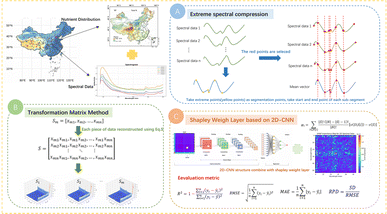
The data used in this study are sourced from the Land Use and Cover Area Frame Survey (LUCAS) soil dataset compiled and released by the Joint Research Centre (JRC) of the European Union. The LUCAS dataset collects soil samples through a scientifically designed composite sampling strategy, with sampling points distributed according to land area and the proportion of land use/cover types in each member state,19 ensuring the representativeness and coverage of the data. The distribution of soil sampling density is shown in Fig. 1, which is downloaded from the JRC website. The LUCAS dataset is a large-scale soil census dataset that has been widely used in recent years for modeling and prediction research concerning soil properties. For example, Panagos et al. used the LUCAS dataset to study soil erodibility across Europe,20 while Pacini et al. developed a method to estimate the organic carbon content in topsoil across agricultural lands in Europe using LUCAS data.21
 |
| | Fig. 1 Soil sampling density distribution. | |
This study used 1665 Finnish soil samples from the LUCAS dataset. The dataset is randomly divided into training, validation, and test sets in a ratio of 6![[thin space (1/6-em)]](https://www.rsc.org/images/entities/char_2009.gif) :2:2. Each sample includes VNIR spectral data ranging from 400 to 2500 nm, with 0.5 nm intervals, yielding 4200 wavelength points per sample. The high spectral resolution provides rich and detailed information for model training and prediction.
:2:2. Each sample includes VNIR spectral data ranging from 400 to 2500 nm, with 0.5 nm intervals, yielding 4200 wavelength points per sample. The high spectral resolution provides rich and detailed information for model training and prediction.
2.2 Methods
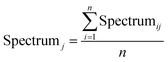
In this study, the proposed 2D-CTM-CNN model overcame the limitations of existing methods through extreme spectral compression, a transformation matrix, and a 2D-CNN combined with a Shapley weight layer. There are three main steps in this method. First, based on the statistical characteristics of VNIR spectral data and their changing trends, the dimensionality of spectral data is significantly reduced while preserving key features. This step prevents excessive data volume in the subsequent 2D transformation, which could decrease computational efficiency. Second, the compressed one-dimensional data are reconstructed into a two-dimensional matrix format, providing the matching input for the 2D-CNN model. Third, a two-dimensional convolutional neural network is then employed to extract deep spectral features. To further enhance the performance of the model, a learnable weighting mechanism based on the Shapley value22,23 is introduced. This mechanism helps the model focus on important regions of the spectral data and improves the prediction accuracy for soil nutrients. An overview of the proposed methods is illustrated in Fig. 2.
 |
| | Fig. 2 The workflow of the 2D-CTM-CNN method. | |
2.2.1 Extreme spectral compression.
The high dimensionality of VNIR spectral data results in strong correlations between adjacent bands and a large amount of redundant information. This increases the risk of overfitting, especially when the number of features exceeds the number of samples. Therefore, dimensionality reduction is essential to improve modeling efficiency, remove noise, and enhance the generalization ability of the prediction model.
The proposed 2D-CTM-CNN model integrates an extreme compression strategy driven by spectral characteristics that efficiently reduce the dimensionality of spectral data. This step automatically selects key spectral points that represent the overall trend and non-linear variations of the original spectral data, enabling substantial dimensionality reduction while preserving important information. Unlike traditional dimensionality reduction methods, this step requires no predefined parameters such as compression ratios or the number of retained features. Therefore, this step eliminates manual intervention, reduces model complexity, and enhances automation and reproducibility by avoiding time-consuming parameter tuning.
The mean vector Spectrumj reflects the global trend of the training dataset, while its peak and valley points correspond to significant trend changes. Thus, these points are used as segmentation locations, dividing the original spectral data into multiple subsegments. Moreover, the data within each subsegment show a consistent directional change, making it easier for the following model to learn the inherent patterns. The equation of Spectrumj is as follows:
| |  | (1) |
where
n is the number of training samples and Spectrum
j is the value of the
ith sample at the
jth wavelength.
After segmentation, it is necessary to select spectral points that can effectively preserve the key information of the original spectral data. For each subsegment, the first and last points are designated as x0 and xn, which are retained as compressed spectral features.
2.2.2 CTM-CNN model.
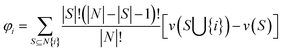
Conventional 1D VNIR spectral data limit the 1D-CNN model's ability to extract complex features across non-adjacent spectral bands, because the convolution kernel can only be slid in one direction. Thus, reconstruction of 1D spectral data into a 2D format enables better capture of spatial structures and spectral relationships. The transformation matrix step is introduced to effectively convert compressed 1D spectral data into a 2D structure suitable for 2D-CNN input. This step can preserve original spectral information and present the inter-point relationships, facilitating effective feature extraction without introducing additional noise. After extreme spectral compression, each sample is represented as Sm = [xm1, xm2, xm3…xmn]. The equation of the transformation matrix is as follows:| | 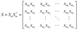 | (2) |
where xmn denotes the nth retained spectral point of the mth spectral data.
Moreover, the normalization operation24 is applied after the generation of the 2D data, constraining all the pixel values to [0, 1]. This not only improves the numerical stability of the transformed data and mitigates the influence of outliers during model training, but also provides compact and representative inputs for the subsequent 2D-CNN model, thereby improving both prediction efficiency and prediction performance.
Although the two-dimensional convolution network is effective in extracting local structural features, it fails to distinguish the relative importance of different regions during feature integration. Since different spectral bands contain varying levels of information related to soil nutrients, the conventional convolution structure treats all regions equally due to weight sharing, lacking the ability to highlight the importance of these vital regions in soil spectral data. To overcome this limitation, this paper introduces a two-dimensional weighting layer based on the Shapley value22 to enhance the model's ability to focus on the important spectral regions. This layer adaptively adjusts the contribution of different feature regions to the final prediction, enabling the model to focus more effectively on the most relevant spectral regions and thereby improving the prediction accuracy. Furthermore, the Shapley value calculation is independent of the subsequent prediction model and only considers the contribution of each feature to the prediction objective, allowing for a more objective evaluation that is not affected by training data bias. To ensure compatibility with the convolutional neural network, this study employs a CNN-based approach to compute the marginal contributions of regions after extracting their local features.
The Shapley value, originating from cooperative game theory, provides a fair and interpretable means of attributing the contribution of individual features to the overall outcome. It can accurately quantify the marginal contribution of each region to the final prediction,25 enabling balanced and transparent feature weighting. In addition to enhancing interpretability by clarifying each feature's influence on prediction outcomes,26 the Shapley value also strengthens the two-dimensional weighting layer to assign differentiated importance to various feature regions. The formulation for computing the Shapley value is provided in eqn (3).
| |  | (3) |
where
φi denotes the Shapley value of the
ith region,
N is the full set consisting of all regions,
S is the subset that does not contain region
i, and
v(
S) denotes the prediction performance of the model under the subset
S.
In this study, a 2D-CNN framework is employed for modeling, integrating conventional convolutional, batch normalization, activation, pooling, and fully connected layers, along with a dynamic weighting layer based on Shapley values. Specifically, the Shapley-based weighting layer is placed before the convolutional operation to adaptively reweight the input spectral features according to their global importance. The convolutional layers utilize sliding kernels to extract spatial relationships and local features from spectral maps, learning region-level combinations and capturing local variations across spectral bands. The batch layer performs normalization on each layer to accelerate the training process, enhancing data stability and alleviating the problem of gradient explosion. The activation layer introduces non-linear feature expression capability to allow the model to capture the complex relationships in the spectral data and enhance the prediction capability. The pooling layers reduce the spatial dimensionality through a downsampling strategy and retain the important features of the data in order to improve computational efficiency and prevent overfitting. Moreover, the Shapley-based weighting layer dynamically identifies and emphasizes important spectral regions, facilitating more focused feature learning. The fully connected layers integrate extracted local features to produce final predictions. During training, the back-propagation algorithm is used to update the model parameters by minimizing the mean squared error (MSE) (eqn (4)),27 which measures the discrepancy between the output of the predicted values and actual nutrient content. Through iterative gradient descent, the model gradually reduces prediction error and achieves automatic feature extraction and regression. Additionally, the Adam optimizer28 is adopted to accelerate convergence and enhance training stability. The network structure is shown in Fig. 3.
| |  | (4) |
where
n denotes the sample size,
yi denotes the true value of the
ith sample, and
ŷi denotes the predicted value of the
ith sample.
 |
| | Fig. 3 2D-CTM-CNN network structure. | |
2.3 Comparison experiments
To rigorously evaluate the prediction accuracy of the proposed 2D-CTM-CNN model, we establish a one-dimensional convolutional neural network, a two-dimensional convolutional neural network combined with the GASF algorithm, a two-dimensional convolutional neural network combined with the MTF algorithm, and PLSR for analysis and comparison. Moreover, a 1D-CNN model based on the CARS (Competitive Adaptive Reweighted Sampling) feature extraction method is also constructed for comparison to validate the effectiveness of the proposed extreme spectral compression step. The comparison models are listed in Table 2.
Table 2 List of comparative models for N and SOC prediction
| Category |
Methods |
Data |
| Linear model |
PLSR |
VNIS |
| 1D-CNN |
1D-CNN |
VNIS |
| 1D-CNN |
Compressed VNIS |
| 1D-CNN |
CARS selected features |
| 2D-CNN |
2D-GASF-CNN |
Compressed VNIS |
| 2D-Markov-CNN |
Compressed VNIS |
| 2D-CTM-CNN |
Compressed VNIS |
2.3.1 PLSR model.
PLSR is a multivariate statistical method that combines features of principal component analysis and multiple linear regression. It is particularly suited for modeling relationships between high-dimensional, collinear, and noisy data, making it widely used in chemometrics and spectral analysis. PLSR projects both predictors and responses into a new latent space, capturing the most relevant variance for prediction.29,30 The spectral data used in this study exhibit strong multicollinearity among variables, with the dimensionality of 4200 and only 1665 samples. This is a typical high-dimensional and small-sample situation that is appropriate for PLSR models. Furthermore, PLSR offers a fast training process and relatively simple parameter tuning compared to more complex nonlinear models, making it a suitable benchmark for performance comparison. In this study, the raw VNIS spectral data are preprocessed using the standard normal variate (SNV)31 before being modeled by PLSR. The number of principal components is varied between 1 and 26, and the prediction results serve as a comparison to evaluate the proposed method.
2.3.2 1D-CNN model.
Convolutional neural networks are a class of feed-forward neural networks capable of automatically extracting features from data in a variety of forms. VNIS data are a continuous string of one-dimensional signals with high local band correlation and strong continuity. Through the use of the sliding convolution kernel, 1D-CNN can effectively extract informative band combination features from raw spectral data and capture the relevant patterns. Compared to linear models, the 1D-CNN models are more effective at capturing non-linear relationships within spectral data and have the advantages of a simpler structure and higher computational efficiency when compared to 2D convolutional neural networks.32
To evaluate the effectiveness of the 2D-CTM-CNN model proposed in this study, the 1D convolutional neural network is used as a comparative model. Both the raw VNIS spectral data and the compressed VNIS spectral data are modeled and predicted using 1D-CNN. This comparison is intended to validate whether the extreme compression step leads to significant information loss in the spectral data and compromises the prediction accuracy of the model. The parameters of the designed 1D-CNN model are shown in Tables 3 and 4, respectively.
Table 3 Parameters of the 1D-CNN for raw spectral data
| Layer |
Input size |
Kernel |
Activation |
Output size |
Parameters |
| Conv1 |
(32, 1, 4200) |
3 |
ReLU |
(32, 32, 4198) |
128 |
| MaxPool1 |
(32, 32, 4198) |
3 |
— |
(32, 64, 1399) |
0 |
| Conv2 |
(32, 64, 1399) |
3 |
ReLU |
(32, 64, 1397) |
6208 |
| MaxPool2 |
(32, 64, 1397) |
3 |
— |
(32, 64, 465) |
0 |
| Conv3 |
(32, 64, 465) |
3 |
ReLU |
(32, 64, 463) |
12352 |
| MaxPool3 |
(32, 64, 463) |
3 |
— |
(32, 64, 154) |
0 |
| Conv4 |
(32, 64, 154) |
3 |
ReLU |
(32, 64, 152) |
12352 |
| MaxPool4 |
(32, 64, 152) |
2 |
— |
(32, 64, 76) |
0 |
| Flatten |
(32, 64, 76) |
— |
— |
(32, 4864) |
0 |
| FC1 |
(32, 4864) |
— |
— |
(32, 128) |
622720 |
| FC2 |
(32, 128) |
— |
— |
(32, 64) |
8256 |
| FC3 |
(32, 64) |
— |
— |
(32, 1) |
65 |
Table 4 Parameters of the 1D-CNN for compressed spectral data
| Layer |
Input size |
Kernel |
Activation |
Output size |
Parameters |
| Conv1 |
32 × 1 × 54 |
3 |
ReLU |
32 × 32 × 52 |
128 |
| MaxPool1 |
32 × 32 × 52 |
3 |
— |
32 × 32 × 17 |
0 |
| Conv2 |
32 × 32 × 17 |
3 |
ReLU |
32 × 32 × 15 |
6208 |
| MaxPool2 |
32 × 32 × 15 |
3 |
— |
32 × 64 × 5 |
0 |
| Flatten |
32 × 64 × 5 |
— |
— |
32 × 320 |
0 |
| FC1 |
32 × 320 |
— |
— |
32 × 128 |
41168 |
| FC2 |
32 × 128 |
— |
— |
32 × 64 |
8256 |
| FC3 |
32 × 64 |
— |
— |
32 × 1 |
65 |
2.3.3 2D-CNN model.
To validate the effectiveness of the proposed 2D-CTM-CNN model, three different 2D convolutional neural network structures are designed and compared: the GASF method combined with 2D-CNN, the Markov transition field (MTF) combined with 2D-CNN, and the 2D-CTM-CNN proposed in this paper. GASF is a two-dimensional encoding technique based on angular transformation. It projects a normalized one-dimensional sequence into a polar coordinate system and constructs a symmetric matrix by computing the pairwise cosine of the angular values, thereby forming a two-dimensional representation that retains temporal trends and the global structure of the time series.33 The GASF transformation is defined by eqn (5). The MTF method is based on state space partitioning and Markov process modeling. It transforms the time series into a two-dimensional image representing the transition probabilities between different states, effectively capturing the dynamic variation characteristics of the sequence. However, this method requires discretizing the numerical sequence into a finite number of states prior to transformation.34 The MTF transformation is described in eqn (6). The two transformation-based 2D-CNN models are used as comparison experiments to evaluate and compare the performance of the proposed 2D-CTM-CNN method. Furthermore, to verify the contribution of the Shapley-based weighting layer, an ablation experiment is conducted by removing this module from the proposed model for comparison. The parameters of the designed 2D-CNN model are shown in Table 5.| | 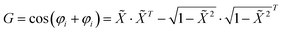 | (5) |
where G denotes the final GASF matrix,  denotes the normalised time series satisfying
 ![[X with combining tilde]](https://www.rsc.org/images/entities/i_char_0058_0303.gif) i ∈ [−1, 1], and φi = cos−1(i) denotes the conversion of the normalised values into angles.
i ∈ [−1, 1], and φi = cos−1(i) denotes the conversion of the normalised values into angles.| | 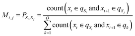 | (6) |
where Mi,j is an element of the Markov transition field matrix, denoting the state transfer probability from time point i to time point j; PSi,Sj is an element of the state transfer probability matrix, denoting the transfer probability from state Si to state Sj; xt ∈ qSi indicates that the data-valued state at time point t belongs to qSi; and Q is the number of states after discretisation.
Table 5 Parameters of the 2D-CNN for compressed spectral data
| Layer |
Input size |
Kernel |
Activation |
Output size |
Parameters |
| Conv1 |
32 × 1 × 54 × 54 |
3 × 3 |
ReLU |
32 × 32 × 52 × 52 |
2916 |
| MaxPool1 |
32 × 32 × 52 × 52 |
2 × 2 |
— |
32 × 32 × 26 × 26 |
0 |
| Conv2 |
32 × 32 × 26 × 26 |
3 × 3 |
ReLU |
32 × 32 × 24 × 24 |
18496 |
| MaxPool2 |
32 × 32 × 24 × 24 |
2 × 2 |
— |
32 × 32 × 12 × 12 |
0 |
| Conv3 |
32 × 32 × 12 × 12 |
3 × 3 |
ReLU |
32 × 32 × 10 × 10 |
73856 |
| MaxPool3 |
32 × 32 × 10 × 10 |
2 × 2 |
— |
32 × 32 × 5 × 5 |
0 |
| Flatten |
32 × 128 × 5 × 5 |
— |
— |
32 × 3200 |
0 |
| FC1 |
32 × 3200 |
— |
— |
32 × 1600 |
5121600 |
| FC2 |
32 × 1600 |
— |
— |
32 × 256 |
409856 |
| FC3 |
32 × 256 |
— |
— |
32 × 64 |
16448 |
| FC4 |
32 × 64 |
— |
— |
32 × 1 |
65 |
2.3.4 Model evaluation.
To evaluate the predictive performance of the proposed model and quantitatively compare the prediction accuracy of different models in predicting SOC and N, several widely used evaluation metrics were used. These include the coefficient of determination (R2; eqn (7)),35 root mean square error (RMSE; eqn (8)),36 mean absolute error (MAE; eqn (9)),37 and the ratio of performance to deviation (RPD; eqn (10)).38 Additionally, the RPD is particularly useful for assessing the practical utility of a prediction model. An RPD value below 1.5 suggests poor predictive performance, values between 1.5 and 2 indicate rough quantitative prediction, values between 2 and 2.5 imply acceptable predictive capability, values between 2.5 and 3 suggest good predictive ability, and values greater than 3 reflect excellent model performance.39| |  | (7) |
| |  | (8) |
| |  | (9) |
| |  | (10) |
where yi denotes the true value of the ith sample, ŷi denotes the predicted value of the ith sample, ȳ denotes the average of the true values of all the samples, n denotes the total number of samples, and SD denotes the standard deviation of the reference value from the true value.
3 Results
3.1 PLSR modeling results
The raw VNIS spectral data were preprocessed using the SNV method to eliminate scatter effects and baseline drift, and the number of principal components was varied from 1 to 26 to explore the impact of dimensionality on the precision of the prediction. The final number of principal components was selected based on the criterion of cumulative explained variance40 to ensure that a sufficient amount of spectral information was retained without overfitting. Cross-validation was used to evaluate the influence of different principal components on the performance of the model. As shown in Table 6, the R2 values are 0.87 for SOC and 0.85 for N and the corresponding RPD values range between 2.5 and 3, indicating a good predictive ability. The results indicate that the PLSR model demonstrates strong predictive and generalization capabilities, effectively retaining the primary spectral features while handling the high dimensionality and multicollinearity inherent in VNIS data. This confirms the suitability of the PLSR model for rapid and reliable soil nutrient prediction.
Table 6 PLSR model performance results for SOC and N estimation
| Property |
Set |
RMSE |
R
2
|
MAE |
RPD |
| SOC |
Training |
50.64 |
0.86 |
37.83 |
2.74 |
| Test |
47.47 |
0.87 |
34.96 |
2.79 |
| N |
Training |
2.24 |
0.86 |
1.52 |
2.66 |
| Test |
2.20 |
0.85 |
1.51 |
2.59 |
3.2 1D-CNN modeling results
The 1D-CNN has demonstrated strong performance in sequential data processing, particularly effective in extracting local patterns and features in spectral data. Thus, it has been widely applied in spectral analysis and regression tasks.41 In this study, a 1D-CNN model is used to extract deep features from VNIS soil spectral data for predicting SOC and N contents. To validate the influence of the extreme compression step in the proposed method, a comparative experiment is conducted. Both the original uncompressed spectral data and the compressed spectral data are used as inputs to independently train 1D-CNN models. The prediction performance of these models is then evaluated and compared to validate whether the dimensionality reduction leads to significant information loss and decreases the precision of the prediction model.
The 1D-CNN model structure used in this experiment consists of three convolutional layers stacked alternately with a pooling layer, followed by the fully connected layer to complete the regression task, in which the hyperparameters such as convolutional kernel size, the number of layers, and the activation function are tuned using stochastic search, Bayesian optimization, etc. Additionally, the training process uses the MSE27 as the loss function and selects the Adam optimizer to facilitate efficient convergence. To prevent overfitting, a dropout layer is introduced into the models and the early stopping strategy is incorporated.
The dimensionality of the spectral data is reduced from 4200 to 54 after the extreme spectral compression step, retaining only 1.29% of the original spectral dimensionality. Nevertheless, the prediction accuracy of the SOC and N does not differ by more than 1%. Compared to the PLSR prediction model, the R2 values of the compressed spectral data prediction model increase by about 3.45% and 4.71%, respectively. Moreover, the RMSE values of SOC and N are reduced by 6.88% and 8.18%, respectively, while the MAE values are reduced by 16.73% and 12.58%, respectively. The PRD increases to more than 3, which indicates that the model has excellent predictive capability. Moreover, a 1D-CNN model based on the CARS feature extraction method is developed for comparison, with the number of sampling iterations set to 50. After CARS-based selection, the number of spectral variables for N is reduced from 4200 to 201 and for SOC from 4200 to 179. The corresponding prediction results are all shown in Table 7. These experimental results demonstrate that the proposed extreme compression step enables simple and effective dimensionality reduction while preserving the essential spectral information necessary for accurate prediction. Furthermore, the 1D-CNN model outperforms the traditional PLSR method, offering superior feature extraction and modeling capabilities, showing that the CNN models are more suitable for predicting soil nutrients.
Table 7 1D-CNN model performance results for SOC and N estimation
| Model |
Property |
Set |
RMSE |
R
2
|
MAE |
RPD |
|
4200 and 54 are the dimensionality of spectral data.
|
| 1D-CNN (4200a) |
N |
Training |
1.92 |
0.89 |
1.28 |
2.92 |
| Test |
2.02 |
0.88 |
1.32 |
2.85 |
| SOC |
Training |
43.64 |
0.90 |
29.11 |
3.41 |
| Test |
44.21 |
0.90 |
29.11 |
3.32 |
| 1D-CNN (54a) |
N |
Training |
2.07 |
0.88 |
1.38 |
2.81 |
| Test |
2.31 |
0.87 |
1.51 |
2.77 |
| SOC |
Training |
53.32 |
0.88 |
34.52 |
2.88 |
| Test |
51.11 |
0.89 |
32.93 |
3.01 |
| 1D-CNN (CARS) |
N |
Training |
2.18 |
0.86 |
1.36 |
2.72 |
| Test |
2.69 |
0.81 |
1.70 |
2.30 |
| SOC |
Training |
57.24 |
0.86 |
35.25 |
2.70 |
| Test |
63.91 |
0.83 |
38.95 |
2.41 |
3.3 2D-CNN modeling results
This study introduces a 2D-CNN-based model for VNIR spectral data analysis to utilize the powerful feature extraction capabilities of the 2D-CNN prediction model. As the compressed spectral data are one-dimensional, they need to be converted into a two-dimensional format to be compatible with the input of the 2D-CNN. To verify the effectiveness and advantages of the proposed method, two widely used time series transformation algorithms (GASF and MTF) are selected for comparison. These comparative experiments aim to evaluate the ability of different transformation methods to preserve critical spectral features and improve the prediction performance. Fig. 4 shows the heat map of the GASF data, the MTF data, and the 2D-CTM data.
 |
| | Fig. 4 Heat maps of different 2D transformations: (a) GASF, (b) MTF, and (c) 2D-CTM. | |
The heat map is a graphical representation of the matrix data, where different color gradients are used to convey the magnitude or intensity of individual values across the matrix.42 From the visual analysis of the heat maps produced by the three transformation methods, it can be observed that each exhibits a certain degree of symmetry. This symmetry implies that the similarity between any two spectral points is preserved bidirectionally, forming a structured pattern that facilitates feature extraction by convolutional neural networks. However, the heat map obtained by the MTF method displays a distinctly block-like and segmented appearance. It lacks smooth transitions and exhibits an interlaced color pattern with weak continuity, making it difficult to capture subtle variations in the spectral data.
This phenomenon may be due to the significant reduction in dimensionality by the extreme compression, resulting in the increase in the probability of the data state transfer and thus affecting the distribution of the converted data. In contrast, heat maps obtained using the GASF method and the proposed method in this paper demonstrate better continuity and coherence. Moreover, the heat map generated by the proposed method shows high-intensity concentration regions in the lower-left corner and along the matrix borders, while the majority of the map retains uniformly low intensity. This structure enables the 2D-CNN model to extract the meaningful spatial features.
This study introduces a Shapley weight layer into the 2D-CNN to enhance the interpretability of the prediction model and quantify the relative importance of each variable in the prediction process after converting the one-dimensional spectral data into a two-dimensional format. The Shapley weight layer serves as an interpretable weighting mechanism that estimates the bounded contribution of each input feature to the output of the prediction model based on the Shapley value. Moreover, the importance of the features through the weight matrix offers insight into how different spectral regions influence the prediction results. Designed as a lightweight and learnable module, the Shapley weight layer is embedded directly within the network architecture and trained jointly with the other model parameters, which ensures that the model achieves high predictive accuracy while maintaining strong interpretability. Fig. 5 presents the normalized Shapley value based on weight matrices for the prediction of SOC and N, respectively. These visualizations highlight the most influential regions in the input space and reinforce the interpretability and practical relevance of the proposed approach.
 |
| | Fig. 5 Weight matrices based on Shapley values: (a) SOC and (b) N. | |
In the weight matrix image, the color of each pixel corresponds to the magnitude of its weight, with darker regions indicating higher importance and lighter regions representing lower importance. The spatial contribution of these weights guides the 2D-CNN prediction model to quickly and effectively identify salient regions and focus on learning the most informative features. In addition, during the training process, the network dynamically adjusts these weights to emphasize critical information, enabling it to focus on key areas rather than treating all regions equally. This adaptive weighting mechanism enhances the efficiency of the prediction model and the predictive accuracy by prioritizing the most relevant spectral region.
Tables 8 and 9 display the modeling performance metrics obtained using the three transformation methods, while Fig. 6 and 7 present the corresponding scatter plots for predicted and actual values of SOC and N, respectively. Based on their performance results, the models can be ranked in order of accuracy as follows: 2D-CTM-CNN model > 2D-GASF-CNN > 2D-MTF-CNN. The proposed 2D-CTM-CNN model outperforms the PLSR, 1D-CNN and two 2D-CNN models. Compared with the 1D-CNN model, the R2 of SOC and N increased by 5.56% and 5.68% and the RMSE reduced by 7.60% and 27.72%, respectively. Furthermore, the PRD for both nutrients exceeds 4, indicating that the model has an excellent prediction ability. These experimental results demonstrated that the proposed method not only achieves substantial dimensionality reduction through extreme spectral compression, but also preserves critical information and enhances feature representation. By introducing a learnable Shapley-based weight matrix into the network architecture, the model is able to focus on the most informative regions of the spectral data. The results of the ablation experiment further confirm the effectiveness of this weighting layer, showing that when the Shapley-based weighting layer is removed, the R2 for N decreases to 0.90 and for SOC to 0.93, indicating that this layer contributes significantly to improving prediction accuracy.
Table 8 Results of estimation of SOC content with different 2D-CNN models
| Model |
Set |
RMSE |
R
2
|
MAE |
RPD |
| 2D-GASF-CNN |
Training |
30.52 |
0.95 |
19.89 |
4.42 |
| Test |
48.60 |
0.89 |
27.28 |
3.08 |
| 2D-MTF-CNN |
Training |
38.60 |
0.93 |
23.77 |
4.01 |
| Test |
98.21 |
0.54 |
62.08 |
1.48 |
| 2D-CTM-CNN |
Training |
29.27 |
0.96 |
18.52 |
4.85 |
| Test |
32.01 |
0.95 |
19.11 |
4.40 |
Table 9 Results of estimation of N content with different 2D-CNN models
| Model |
Set |
RMSE |
R
2
|
MAE |
RPD |
| 2D-GASF-CNN |
Training |
1.55 |
0.92 |
1.31 |
3.89 |
| Test |
2.10 |
0.87 |
1.68 |
2.79 |
| 2D-MTF-CNN |
Training |
1.55 |
0.93 |
1.36 |
3.84 |
| Test |
4.15 |
0.46 |
2.64 |
1.36 |
| 2D-CTM-CNN |
Training |
1.36 |
0.94 |
1.02 |
4.36 |
| Test |
1.48 |
0.93 |
1.09 |
4.06 |
 |
| | Fig. 6 Scatter plot of the measured and predicted concentrations of SOC of the Finnish dataset: (a) training set of 2D-GASF-CNN, (b) training set of 2D-MTF-CNN, (c) training set of 2D-CTM-CNN, (d) test set of 2D-GASF-CNN, (e) test set of 2D-MTF-CNN, and (f) test set of 2D-CTM-CNN. | |
 |
| | Fig. 7 Scatter plot of the measured and predicted concentrations of N of the Finnish dataset: (a) training set of 2D-GASF-CNN, (b) training set of 2D-MTF-CNN, (c) training set of 2D-CTM-CNN, (d) test set of 2D-GASF-CNN, (e) test set of 2D-MTF-CNN, and (f) test set of 2D-CTM-CNN. | |
This mechanism significantly improves the interpretability and efficiency of the training process, which results in more accurate and robust prediction results. Nevertheless, the 2D-GASF-CNN and 2D-MTF-CNN exhibit the problem of overfitting, which is likely attributed to the non-isometric compression that influences the structure of original spectral data. This disruption negatively impacts the effectiveness of the time-series-based encoding methods that limits the suitability for high-dimensional spectral after the extreme spectral compression step. Additionally, the performance of the 2D-MTF-CNN model is particularly sensitive to the n_state parameter, which controls the discretization of continuous spectral values into finite states. When applied to low-dimensional data, this discretization reduces the representational granularity of the transformed matrix, limits the learning capacity of the prediction model, and leads to suboptimal prediction performance.
3.4 Generalization validation results
To further assess the generalization and robustness of the proposed 2D-CTM-CNN model, additional validation experiments were conducted using other datasets and soil properties. Specifically, the Italy dataset containing 1180 samples was employed to evaluate the model's applicability for predicting nitrogen (N) and soil organic carbon (SOC). Furthermore, two additional soil properties were included to examine the model's adaptability to different nutrient types: cation exchange capacity (CEC) from the Finnish dataset and calcium carbonate (CaCO3) from the Italy dataset. In these experiments, the predictive performance of the proposed 2D-CTM-CNN model was compared with that of a one-dimensional full-spectrum convolutional model. The 1D-CNN and 2D-CNN architectures employed in this validation were identical to those used in the previous experiments, ensuring a consistent and fair comparison.
Table 10 shows the prediction performance of SOC and N in the Italian dataset using the full-spectrum 1D-CNN and the proposed 2D-CTM-CNN. The 2D-CTM-CNN consistently outperformed the 1D-CNN on both training and testing sets. For N, the test set R2 increased from 0.48 to 0.68 (41.7% improvement) and RMSE decreased from 0.98 to 0.80. For SOC, R2 increased from 0.56 to 0.73 (30.4% improvement) with RMSE reducing from 12.57 to 9.56. These results indicate that the 2D-CTM-CNN effectively captures spectral patterns relevant to SOC and N and exhibits strong generalization across different soil datasets.
Table 10 Results for SOC and N estimation of the Italy dataset
| Model |
Property |
Set |
RMSE |
R
2
|
MAE |
RPD |
| 1D-CNN |
N |
Training |
0.77 |
0.64 |
0.51 |
1.68 |
| Test |
0.98 |
0.48 |
0.58 |
1.50 |
| SOC |
Training |
9.01 |
0.78 |
5.90 |
2.16 |
| Test |
12.57 |
0.56 |
6.96 |
1.52 |
| 2D-CTM-CNN |
N |
Training |
0.54 |
0.83 |
0.36 |
2.43 |
| Test |
0.80 |
0.68 |
0.47 |
1.77 |
| SOC |
Training |
7.21 |
0.85 |
4.93 |
2.59 |
| Test |
9.56 |
0.73 |
6.16 |
1.94 |
Table 11 presents the prediction performance for CEC and calcium carbonate (CaCO3). The 2D-CTM-CNN showed clear advantages over the 1D-CNN for both training and testing sets. For CEC, the test set R2 improved from 0.66 to 0.96 (45.5% improvement) with RMSE decreasing from 7.72 to 2.20, while for CaCO3, R2 increased from 0.71 to 0.77 and RMSE decreased from 76.53 to 63.59. Fig. 8 shows that predictions from the 2D-CTM-CNN are closer to the ideal y = x line, demonstrating higher accuracy and reliability. Overall, the proposed model effectively captures complex spectral patterns across multiple soil properties and exhibits broad applicability for robust soil property prediction.
Table 11 Results for CEC and CaCO3 estimation
| Model |
Property |
Set |
RMSE |
R
2
|
MAE |
RPD |
| 1D-CNN |
CEC |
Training |
6.72 |
0.70 |
4.32 |
1.89 |
| Test |
7.72 |
0.66 |
4.57 |
1.69 |
| CaCO3 |
Training |
55.59 |
0.84 |
39.18 |
2.56 |
| Test |
76.53 |
0.71 |
52.75 |
1.85 |
| 2D-CTM-CNN |
CEC |
Training |
2.47 |
0.96 |
1.68 |
5.31 |
| Test |
2.20 |
0.96 |
1.48 |
5.01 |
| CaCO3 |
Training |
49.95 |
0.87 |
33.94 |
2.78 |
| Test |
63.59 |
0.77 |
42.49 |
2.11 |
 |
| | Fig. 8 Scatter plot of the measured and predicted concentrations of CaCO3 and CEC: (a) 1D-CNN of CaCO3, (b) 2D-CTM-CNN of CaCO3, (c) 1D-CNN of CEC, and (d) 2D-CTM-CNN of CEC. | |
4 Conclusion
This study demonstrated the effectiveness of the proposed lightweight two-dimensional convolutional neural network (2D-CTM-CNN) for accurate estimation of SOC and N content. The model reduced spectral dimensionality from 4200 to 54 while incorporating a Shapley value-based weighting layer, which significantly enhanced predictive performance. Compared with baseline models, R2 values for SOC and N improved by 5.56% and 5.68%, respectively, while RMSE decreased by 7.60% and 27.72%. In addition, relative prediction deviation (RPD) values for both nutrients exceeded 4, confirming excellent predictive capacity. Thus, the proposed framework eliminates the need for extensive preprocessing by directly operating on compressed spectral data, thereby simplifying the modeling process without compromising accuracy. The advantages of this lightweight design enable fast, accurate, and interpretable prediction of soil nutrient content, underscoring its potential for precision agriculture. Future research will focus on integrating multi-source data into the 2D-CTM-CNN framework to further enhance robustness and generalization across diverse environmental conditions.
Author contributions
Feng X.: supervision, writing review, and investigation; Ma X. Y.: conceptualization, investigation, writing – original draft, and writing – editing; Yang H. W.: supervision, writing – review, and funding acquisition; Zhang J.: supervision and writing – review.
Conflicts of interest
There are no conflicts to declare.
Data availability
All the data used in this study are from LUCAS, using publicly available data at [http://esdac.jrc.ec.europa.eu/].
Acknowledgements
This work was supported by the Department of Agriculture and Rural Affairs of Jilin Province (KYC-JC-XM-2024-245).
References
- S. J. Leghari, N. A. Wahocho, G. M. Laghari, A. HafeezLaghari, G. MustafaBhabhan, K. HussainTalpur, T. A. Bhutto, S. A. Wahocho and A. A. Lashari, Adv. Environ. Biol., 2016, 10, 209–219 Search PubMed.
- F. Mahmood, I. Khan, U. Ashraf, T. Shahzad, S. Hussain, M. Shahid, M. Abid and S. Ullah, J. Plant Nutr. Soil Sci., 2017, 17, 22–32 Search PubMed.
- X. Zhang, Y. Zhao and E. Xie,
et al.
, J. Agro-Environ. Sci., 2020, 39, 673–679 Search PubMed.
- Q. Xiao, N. Wu, W. Tang, C. Zhang, L. Feng, L. Zhou, J. Shen, Z. Zhang, P. Gao and Y. He, Front. Plant Sci., 2022, 13, 1080745 CrossRef CAS PubMed.
- M. S. Luce, N. Ziadi and R. A. V. Rossel, Geoderma, 2022, 425, 116048 CrossRef.
- D. Wang, F. Zhao, R. Wang, J. Guo, C. Zhang, H. Liu, Y. Wang, G. Zong, L. Zhao and W. Feng, Front. Plant Sci., 2023, 14, 1138693 CrossRef PubMed.
- H. A. Noreldeen, K.-Y. Huang, G.-W. Wu, H.-P. Peng, H.-H. Deng and W. Chen, Anal. Chem., 2022, 94, 9287–9296 CrossRef CAS PubMed.
- B. Wang, J. Deng and H. Jiang, Foods, 2022, 11, 2210 CrossRef CAS PubMed.
- R. Li, B. Yin, Y. Cong and Z. Du, Sensors, 2020, 20, 6271 CrossRef CAS PubMed.
-
M. Veres, G. Lacey and G. W. Taylor, Proceedings of the 12th Conference on Computer and Robot Vision, New York, NY, USA, 2015, pp. 8–15 Search PubMed.
- J. Padarian, B. Minasny and A. McBratney, Geoderma Reg., 2019, 16, e00198 CrossRef.
- M. S. Rashid, Y. Wang, Y. Yin, B. Yousaf, S. Jiang, A. F. Mirza, B. Chen, X. Li and Z. Liu, Toxics, 2024, 12, 535 CrossRef CAS PubMed.
- X. Fan, X. Feng, Y. Dong and H. Hou, Displays, 2022, 72, 102150 CrossRef CAS PubMed.
- B. Hu, W. Jiang, J. Zeng, C. Cheng and L. He, Front. Plant Sci., 2023, 14, 1231903 CrossRef PubMed.
- J. Yue, H. Yang, H. Feng, S. Han, C. Zhou, Y. Fu, W. Guo, X. Ma, H. Qiao and G. Yang, Comput. Electron. Agric., 2023, 211, 108011 CrossRef.
- J. Deng, X. Liu, G. Du, X. Yang, L. Jiang and C. Sun, Sci. Rep., 2025, 15, 4619 CrossRef CAS PubMed.
- A. Tang, G. Yang, Z. Li, Y. Pan, Y. Liu, H. Long, W. Chen, J. Zhang, Y. Yang and X. Yang,
et al.
, Comput. Electron. Agric., 2025, 231, 109986 CrossRef.
- D. Peng, R. Xu, Q. Zhou, J. Yue, M. Su, S. Zheng and J. Li, Molecules, 2023, 28, 5728 CrossRef CAS PubMed.
- A. Orgiazzi, C. Ballabio, P. Panagos, A. Jones and O. Fernández-Ugalde, Eur. J. Soil Sci., 2018, 69, 140–153 CrossRef.
- P. Panagos, K. Meusburger, C. Ballabio, P. Borrelli and C. Alewell, Sci. Total Environ., 2014, 479, 189–200 CrossRef PubMed.
- L. Pacini, P. Arbelet, S. Chen, A. Bacq-Labreuil, C. Calvaruso, F. Schneider, D. Arrouays, N. P. Saby, L. Cécillon and P. Barré, Sci. Total Environ., 2023, 900, 165811 CrossRef CAS PubMed.
- Y. Ning, M. E. H. Ong, B. Chakraborty, B. A. Goldstein, D. S. W. Ting, R. Vaughan and N. Liu, Patterns, 2022, 3, 100452 CrossRef PubMed.
- J. Mercik, B. Gładysz, I. Stach and J. Staudacher, Entropy, 2021, 23, 1598 CrossRef PubMed.
- M. Akhavanfar, T. K. Uchida and R. B. Graham, J. Biomech., 2023, 147, 111441 CrossRef PubMed.
- J. Sun, H. Yu, G. Zhong, J. Dong, S. Zhang and H. Yu, IEEE Trans. Cybern., 2020, 52, 205–214 Search PubMed.
- M. F. Hosen, S. H. Mahmud, K. Ahmed, W. Chen, M. A. Moni, H.-W. Deng, W. Shoombuatong and M. M. Hasan, Comput. Biol. Med., 2022, 145, 105433 CrossRef CAS PubMed.
- S. Volcevska, L. Luck, R. Elmir, G. Dickens and G. Murphy, Int. J. Ment. Health Nurs., 2024, 33, 224–240 Search PubMed.
- C. Wang, J. Ma, G. Wei and X. Sun, Sensors, 2025, 25, 661 CrossRef PubMed.
- A. Carlier, S. Dandrifosse, B. Dumont and B. Mercatoris, Front. Plant Sci., 2023, 14, 1204791 CrossRef PubMed.
- M. Metz, F. Abdelghafour, J.-M. Roger and M. Lesnoff, Anal. Chim. Acta, 2021, 1179, 338823 CrossRef CAS PubMed.
- B. Li, L. Yu and L. Gao, Comput. Biol. Med., 2022, 151, 106270 CrossRef PubMed.
- R. Noda, D. Ichikawa and Y. Shibagaki, Sci. Rep., 2024, 14, 12426 CrossRef CAS PubMed.
- X. Ye, Y. Huang, Z. Bai and Y. Wang, Front. Physiol., 2023, 14, 1174525 CrossRef PubMed.
- W. Sun, J. Zhou, B. Sun, Y. Zhou and Y. Jiang, Micromachines, 2022, 13, 873 CrossRef PubMed.
- N. Hunter, M. Rahbar, R. Wang, M. Mahjouri-Samani and X. Wang, Opt. Lett., 2022, 47, 6357–6360 CrossRef CAS PubMed.
- K. Serefoglu Cabuk, S. K. Cengiz, M. G. Guler, H. Topcu, A. Cetin Efe, M. G. Ulas and F. Poslu Karademir, Int. Ophthalmol., 2024, 44, 303 CrossRef PubMed.
- Z. Xu, Y. Dai, F. Liu, W. Chen, Y. Liu, L. Shi, S. Liu and Y. Zhou, Comput. Biol. Med., 2023, 161, 107037 CrossRef PubMed.
- M. Awawdeh, M. B. Alotaibi, A. H. Alharbi, S. A. Alnafisah, T. S. Alasiri, N. I. Alrashidi and S. A. Alnafisah,
et al.
, Cureus, 2024, 16, 51793 Search PubMed.
- S. Chaturvedi, N. M Alqahtani, M. A Al-Qarni, S. M Alqahtani, G. Suleman, A. Yaqoob, M. Abdul Khader, A. Elsir Elmahdi and M. Chaturvedi, BMC Oral Health, 2024, 24, 1–14 CrossRef PubMed.
- M. Shinn, Proc. Natl. Acad. Sci. U. S. A., 2023, 120, e2311420120 CrossRef CAS PubMed.
- M. Hedyehzadeh, K. Maghooli, M. MomenGharibvand and S. Pistorius, J. Digit. Imag., 2020, 33, 391–398 CrossRef PubMed.
- F. Willer, Health Promot. J. Aust., 2024, 35, 293–302 CrossRef PubMed.
|
| This journal is © The Royal Society of Chemistry 2026 |
Click here to see how this site uses Cookies. View our privacy policy here. 
 b,
Xiaoyuan
Ma
b,
Xiaoyuan
Ma


 denotes the normalised time series satisfying


