DOI:
10.1039/D5SM00947B
(Paper)
Soft Matter, 2025,
21, 8711-8723
Ring polymers in two-dimensional melts double-fold around randomly branching “primitive shapes”
Received
18th September 2025
, Accepted 24th October 2025
First published on 27th October 2025
Abstract
Drawing inspiration from the concept of the “primitive path” of a linear chain in melt conditions, we introduce here a numerical protocol which allows us to detect, in an unambiguous manner, the “primitive shapes” of ring polymers in two-dimensional melts. Then, by analysing the conformational properties of these primitive shapes, we demonstrate that they conform to the statistics of two-dimensional branched polymers (or, trees) in the same melt conditions, in agreement with seminal theoretical work by Khokhlov, Nechaev and Rubinstein. Results for polymer dynamics in light of the branched nature of the rings are also presented and discussed.
1 Introduction
Edwards introduced the concept of a “primitive path” long ago1 to explain the viscoelastic behavior of entangled polymer solutions and melts (see panel (a) of Fig. 1). This idea has since become a cornerstone of polymer physics. In a polymer melt the motion of each chain is constrained by its neighbors, which perform as uncrossable, topological obstacles caging the chain within a tube-like region.2 The primitive path represents the central axis of this tube, and it is identified as the shortest path which the polymer chain can be contracted into, at fixed chain ends and without crossing the topological obstacles represented by the surrounding chains or each other.3,4 This definition, when applied to computer-generated conformations of entangled linear polymer melts,5 allows researchers to map a melt of polymer chains into a melt of primitive paths. Quite remarkably, this mapping provides a universal framework6 for describing the macroscopic rheological properties of entangled polymer liquids, regardless of their specific chemical composition.
 |
| | Fig. 1 (a) Classical illustration of the primitive path (dashed line) of a linear chain (solid line) in an entangled polymer melt. By representing the effects of the constraints exerted by neighboring chains as a network of uncrossable topological obstacles (×), the primitive path is identified as the shortest path which the polymer chain can be contracted into, at fixed chain ends and without crossing the obstacles. (b) In a melt of unknotted and non-concatenated rings, the equivalent topological barriers induce each ring to double-fold around a randomly branching path. | |
The conventional definition of a primitive path is intuitive and simple, but it relies on the presence of free chain ends. This raises a problem: can this concept be generalized to entangled polymers with no free ends?
In this work we explore this question by considering melts of unknotted and non-concatenated ring polymers, a particular class of systems that has challenged theorists,7–17 experimentalists18–23 and computational24–31 physicists for decades. In particular, Khokhlov and Nechaev7 and Rubinstein and coworkers8,10 suggested that, because of the constraint of non-concatenation, rings minimize their mutual overlap by double-folding around randomly branching, or tree-like, primitive paths (see panel (b) of Fig. 1).
The main goal of this work is to provide a direct numerical test of the Khokhlov–Nechaev–Rubinstein picture. Specifically, we introduce a numerical algorithm to straightforwardly and unambiguously extract the primitive path (to which, to distinguish it from the primitive path of linear chains, we prefer from now on the term “primitive shape”) of rings in two-dimensional computer-generated melts. Our results show that these primitive shapes exhibit complex, non-trivial behavior which is, indeed, strongly reminiscent of branched, tree-like conformations. To demonstrate that, we present a detailed characterization of their statistical properties using the set of observables and distribution functions previously introduced by one of us (A.R.) and R. Everaers32–34 for studying two- and three-dimensional lattice trees in various dilution conditions.
The paper is organized as follows. In Section 2.1 we introduce the polymer model and the kinetic Monte Carlo algorithm used for the numerical simulations of ring melts, in Section 2.2 we provide details on the simulated systems, while in Section 2.3 we describe the algorithm used to reconstruct the primitive shape of each ring. Section 3 is devoted to recapitulate the relevant state-of-the-art theoretical ideas describing the structure of interacting random trees, focusing in particular on observables (Section 3.1) and distribution functions (Section 3.2). In Section 4 we present the main results, where we frame the extracted primitive shapes of rings in terms of the theoretical ideas for 2d melts of random trees. Then (Section 5), we discuss these results at the light of ring dynamics, highlighting in particular the fact that 2d rings represent a quite special situation with respect to 3d rings. Outlook and conclusions are presented in Section 6.
2 Polymer model, simulation methods, analysis of polymer conformations
2.1 Kinetic Monte Carlo algorithm
We adapt the efficient kinetic Monte Carlo (MC) algorithm employed in31,35–37 to construct equilibrated dense melts of self-avoiding ring polymers on the two-dimensional triangular lattice (see Fig. 2). The lattice spacing, denoted by a, is chosen as the reference unit of length. The algorithm, based on the elastic lattice polymer model analogous to the Rubinstein's repton model,38 works as the following. Two consecutive monomers along the chain can either sit on nearest neighbour lattice sites or occupy the same lattice site, with strictly no more than two monomers on the same site. At the same time, double occupancy of the same site by non-consecutive monomers is not permitted due to excluded volume. As such, the bond length b between nearest neighbor monomers takes the two possible values, = a or = 0, and in the latter case the bond is said to host a unit of stored length. For a generic ring polymer with Nring bonds, the total contour length Lc ≡ Nring〈b〉 < Nringa where 〈b〉 is the average bond length. This numerical “trick” makes the polymer elastic.
 |
| | Fig. 2 Two-dimensional illustration of the lattice polymer model and kinetic Monte Carlo moves. Monomers (filled dots) occupy the spatial positions of the regular triangular lattice (empty dots) and two nearest neighbor monomers are connected by a black line representing the polymer bond between them. For two nearest neighbor monomers occupying the same lattice site the bond that connects them (represented by an arc) represents a unit of “stored length”. Lattice positions connected by the double arrows are examples of allowed MC moves: (i) a unit of stored length unfolding to a normal bond, (ii) a bond folding into a unit of stored length, (iii) a Rouse-like move. Lattice positions connected by the double arrows with the cross are examples of forbidden MC moves: (iv) a monomer moving to the left that would occupy a lattice position with two monomers already present, (v) two non-nearest neighbor monomers on the same lattice site violating the excluded volume constraint. | |
To explore the effects of chain composition, we have considered polymer chains of different stiffnesses which have been modelled by introducing the following energy penalty term31,
| | 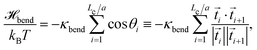 | (1) |
for bending, where
κbend represents the bending stiffness parameter and
![[t with combining right harpoon above (vector)]](https://www.rsc.org/images/entities/i_char_0074_20d1.gif) i
i ≡
![[r with combining right harpoon above (vector)]](https://www.rsc.org/images/entities/i_char_0072_20d1.gif) i+1
i+1 −
i is the oriented bond vector between monomers
i and
i + 1 having spatial coordinates
i and
i+1.
† It should be noticed that, since bond vectors are obviously ill-defined when two monomers form a stored length, the sum in
eqn (1) is restricted to the effective bonds of the chains. By increasing
κbend, the energy term
eqn (1) makes polymers stiffer.
Ring polymers are let to evolve in time, and thus reach equilibrium, by proposing moves that obey the occupancy constraints described above. In more detail, a single move consists in randomly picking a monomer of one of the chains in the system and attempting its displacement towards one of the nearest lattice sites (see Fig. 2 for an illustration of possible situations that may occur). As in ref. 31, the move is then accepted based on the standard Metropolis–Hastings criterion39 taking into account the energy term eqn (1) and with the additional constraints of maintaining chain connectivity and that the destination lattice site is either (1) empty or (2) occupied at most by one of the nearest neighbor monomers along the chain. In analogy with classical37,40,41 polymer dynamics, case (1) is an example of Rouse-like move while case (2) is a reptation-like move (essentially the move produces mass drift along the contour length of the chain, as occurring in reptation dynamics). By these two moves only, the algorithm reproduces known40,41 features of polymer dynamics and, thanks to the stored length “trick” which integrates local fluctuations of the chain density, remains efficient even when it is applied to the equilibration of very dense systems.36
2.2 Simulation details
We have considered bulk solutions of M closed (ring) polymer chains, each chain made of Nring monomers or bonds, with values Nring × M = [40 × 1920, 80 × 960, 160 × 480, 320 × 240, 640 × 120, 1280 × 60], with constant total number of monomers = 76![[thin space (1/6-em)]](https://www.rsc.org/images/entities/char_2009.gif) 800. Bulk conditions are implemented through the enforcement of periodic boundary conditions in a simulation box of total surface S, where the linear sizes of the box, equal to
800. Bulk conditions are implemented through the enforcement of periodic boundary conditions in a simulation box of total surface S, where the linear sizes of the box, equal to  has been fixed based on the monomer number density
  that guarantees melt conditions. All these systems have been studied for bending stiffness parameters κbend = 0, 1, 1.5 (eqn (1)). For completeness, we report the measured MC acceptance rate as a function of the chain stiffness: 0.125 (κbend = 0), 0.021 (κbend = 1), 0.018 (κbend = 1.5). Notice that they are in line with the reported31 acceptance rates for 3d ring melts.
Each system is initialized by arranging the rings inside the simulation box in a conformation that avoids unphysical overlaps between monomers and nested states. To achieve this goal, the initial condition consisted of a melt of M randomly generated, linear, self-avoiding walks of total number of monomers Nring/2. Then, we arrange ring monomers 1 and Nring on the spatial position of one of the walk's ends, and continue by placing ring monomers 2 and Nring − 1 on the next node of the walk, and so on until we get a perfectly, tightly double-folded ring conformation. Following this, we remove any residual overlap between ring monomers by performing a short kinetic Monte Carlo relaxation run. This procedure ensures that in the beginning configuration each ring is both self-avoiding and non-overlapping with the other rings of the melt while preserving local chain connectivity.
Then, for each MC step we pick a single monomer at random, displace it towards a random lattice neighbor and check if the move satisfies the constraints as described in Section 2.1. By taking as unit of “time” 1 MC sweep ≡ (Nring×M) MC steps = 76800 MC steps, we run simulations for ≃107 up to ≃108 MC sweeps. Notice that the length of each individual run is much larger than the characteristic relaxation time of the chain (see definition eqn (30) in Section 5), that guarantees complete equilibration of the chains (see Table S1 in SI). To graphically illustrate this point, we monitor chain relaxation to equilibrium in terms of the monomer mean-square displacement relative to the chain center of mass42,
| | 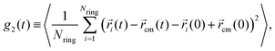 | (2) |
where
. Asymptotically,
g2(
t→∞) = 2〈
Rg2〉
ring where
| | 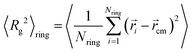 | (3) |
is the ring mean-square gyration radius. The appearance of a plateau in the large-time behavior of
g2 (see Fig. S1 in SI) is the signature that our chains have attained complete structural relaxation.
2.3 Reconstructing the primitive shapes of ring polymers: algorithmic definition
We reconstructed the primitive shapes of individual ring polymer configurations in a 2d melt configuration by introducing a numerical algorithm based on the original intuitions of Khokhlov and Nechaev7 and Rubinstein,8,10 according to which each ring polymer behaves like being confined in a lattice of fixed obstacles (representing all the surrounding rings in the melt) and it can be mapped then onto a tree-like structure on the corresponding dual lattice where such obstacles are absent.
In our simulations polymers reside on the 2d triangular lattice of reference unit step = a, whose dual is the honeycomb lattice (panel (a) of Fig. 3) of unit step  . For each ring in a typical melt configuration (panel (b) of Fig. 3), we identified first the honeycomb lattice sites residing within its contour which allow us to identify, without ambiguity, the nodes of the associated “backbone”. Then, we connect any two of these nodes of the honeycomb lattice by an edge whenever they are spatial nearest neighbors. Visual inspection on the obtained conformations (black lines in panel (c) of Fig. 3) confirms indeed a pronounced tree-like architecture.
 |
| | Fig. 3 (a) Illustration of the 2d triangular lattice (orange dots, with 6 unit cells drawn explicitly) of unit step = a where ring polymers are simulated, along with the dual honeycomb lattice (blue dots, with 1 cell drawn explicitly) of unit step  where the corresponding trees reside. (b) Snapshots of ring melt configurations for Nring = 1280 and κbend = 0, 1, 1.5 (from left to right, see legend). (c) Examples of single ring polymers (blue/green/red circular contours) isolated from their corresponding melts, along with their primitive tree-like backbones (black lines inside each circular contour). Notice that the trees contain a certain amount of loops. (d) Final, loop-less, primitive shapes obtained by randomly removing one bond in each of the former loops. Shown on the l.h.s. of the figure, zoomed-in selected portions of tree conformations for κbend = 0 with loops and without loops after bonds removal. where the corresponding trees reside. (b) Snapshots of ring melt configurations for Nring = 1280 and κbend = 0, 1, 1.5 (from left to right, see legend). (c) Examples of single ring polymers (blue/green/red circular contours) isolated from their corresponding melts, along with their primitive tree-like backbones (black lines inside each circular contour). Notice that the trees contain a certain amount of loops. (d) Final, loop-less, primitive shapes obtained by randomly removing one bond in each of the former loops. Shown on the l.h.s. of the figure, zoomed-in selected portions of tree conformations for κbend = 0 with loops and without loops after bonds removal. | |
If a ring was perfectly double-folded, the resulting tree backbone would be, by construction, without closed loops. In our simulated structures, a non-null amount of loops per ring is however always found (panel (c) of Fig. 3 and the zoomed-in portion for κbend = 0 on the l.h.s.). On the other hand, after easily verifying that such an amount remains small, essentially one may assume that loops do not compromise in any fundamental manner the statistical description of the trees, only they would make the analysis of tree conformations technically harder. For these reasons, we introduce the rule of removing loops simply by randomly cutting one bond of each of them (panel (d) of Fig. 3 and the zoomed-in portion for κbend = 0 on the l.h.s.). As anticipated the fraction of removed bonds is small, at most ≃8% for κbend = 1.5 of the original looped conformations (see Fig. S2 in SI).
2.4 Trees analysis
Each reconstructed tree is made of a total number of “honeycomb-lattice” nodes Ntree which, on average, is equal to ≃80% of the original number of “triangular-lattice” nodes Nring of each ring (l.h.s. panel of Fig. S3 in SI).
As a consequence of the properties of the honeycomb lattice, every tree node may have one, two or, at most, three bonds protruding from it;‡ in the last case, we call that node a “branch-node”. Interestingly, we have found that the mean fraction of branch-nodes depends on the original ring stiffness κbend, with flexible rings being sensibly more branched than stiffer rings. Indeed, as shown in the r.h.s. panel of Fig. S3 in SI, the amount of branch-nodes saturates in the asymptotic limit of large rings (i.e., trees) from ≃22% for κbend = 0 up to ≃13% for κbend = 1.5.
After reconstructing the coordinates and bond connectivities of the ring primitive shapes, we have analyzed tree connectivity and spatial structure by using the “burning” algorithm for trees originally introduced in ref. 32. This algorithm works iteratively: each step consists in removing from the list of all tree nodes those with only one bond protruding from it and updating the number of bonds and the indices of the remaining ones accordingly. The algorithm stops when only one node (the so called “center” of the tree) remains in the list. In this way, by keeping track of the nodes that have been removed, it is possible to obtain information about the mass and the shape of tree branches (Section 3.1.1). The algorithm can be then generalized to detect also the minimal path length ![[small script l]](https://www.rsc.org/images/entities/char_e146.gif) ij between any pair of nodes i and j (Section 3.1.1): it is in fact sufficient that both nodes “survive” the burning process. For a more detailed illustration of the burning algorithm and of its applications on trees, see ref. 32–34.
ij between any pair of nodes i and j (Section 3.1.1): it is in fact sufficient that both nodes “survive” the burning process. For a more detailed illustration of the burning algorithm and of its applications on trees, see ref. 32–34.
3 Structure of two-dimensional melts of branched polymers: theory and methods
In this Section, we introduce quantities and methods of analysis that will be used (in Section 4) to characterize the tree-like conformational properties of the ring primitive shapes.
3.1 Observables
3.1.1 Definitions.
To explore the connection between the primitive shape of our 2d rings and the physics of branched polymers, we follow closely the works32,33 and discuss the power-law behaviors for the following observables:
1. The mean path length as a function of the mean tree weight 〈Ntree〉§:
where
and
ij is the minimal path length connecting the pair of nodes
i and
j on a tree of weight =
Ntree.
2. The mean branch weight as a function of the mean tree weight 〈Ntree〉:
where
Nbr ≡ min(
n,
Ntree − 1 −
n) is the weight of the smallest of the two sub-trees that are obtained by cutting one tree bond.
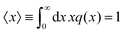
3. The mean-square end-to-end spatial distance as a function of the mean path length 〈L〉:
4. The tree mean-square gyration radius as a function of the mean tree weight 〈Ntree〉:
where
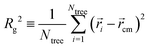
and

is the spatial position of the tree center of mass.
Notice the fundamental relations ρ = ε44 and ν = ρνpath32,33 holding between exponents. The complete list of the measured mean values with corresponding error bars for the different ring systems is presented in Table S2 in SI.
3.1.2 Extrapolation of exponents from data for finite-size trees.
In order to get reliable values and errors of scaling exponents “ρ, ε, νpath, ν” in the asymptotic (i.e., 〈Ntree〉 → ∞) limit, we adopt the following strategy, similar to the one employed in previous works,32,33 which combines together the results obtained from fitting the 〈Ntree〉-dependent data to two functional forms.
To fix the ideas, take the data for the observable 〈Rg2〉 as a function of 〈Ntree〉 and the corresponding exponent ν and use the following expressions:
1. A simple power-law behavior with two (c, ν) fit parameters:
| | | log(〈Rg2〉) = 2νlog(〈Ntree〉) + c, | (8) |
which we use only on the data with
Nring ≥ 320 (namely for the three largest rings/trees).
2. A power-law behavior with a correction-to-scaling term and four (c, d, Δ, ν) fit parameters:
| |  | (9) |
which we use on the entire
Nring-range.
For the other exponents, analogous expressions to eqn (8) and (9) have been employed. In all cases, best fit parameters were obtained by standard χ2-minimization. The results of the two- (eqn (8)) and four-parameter (eqn (9)) fits are collected in Table S3 in SI. Overall the two procedures lead to similar results for the scaling exponents; we combine then the two results together as:
| |  | (10) |
to obtain a final estimate and the corresponding error bar. See
Table 1 for summary, and for comparison with the reference values of the exponents for 2d tree melts reported in
ref. 33.
Table 1 Exponents characterizing tree observables (column 1) and relations between them (column 2, see ref. 33 for details). Column 3 reports the values for 2d tree melts estimated in ref. 33. Columns 4 to 6 report the estimated values for the tree-like primitive shapes of the 2d ring melts considered in this work, for different ring bending stiffness κbend. For technical details on the derivation of these exponents, see Section 3.1.2
|
|
Relation to other exponents33 |
Measured value (ref. 33) |
Measured value (this work) |
|
κ
bend = 0 |
κ
bend = 1 |
κ
bend = 1.5 |
| 〈L〉 ∼ 〈Ntree〉ρ |
— |
0.613 ± 0.007 |
0.63 ± 0.04 |
0.61 ± 0.05 |
0.59 ± 0.07 |
| 〈Nbr〉 ∼ 〈Ntree〉ε |
ε = ρ |
0.63 ± 0.01 |
0.64 ± 0.05 |
0.63 ± 0.04 |
0.63 ± 0.03 |
| 〈Rpath2〉 ∼ 〈L〉2νpath |
— |
0.780 ± 0.005 |
0.783 ± 0.006 |
0.79 ± 0.02 |
0.687 ± 0.006 |
| 〈Rg2〉 ∼ 〈Ntree〉2ν |
ν = ρνpath |
0.48 ± 0.02 |
0.50 ± 0.02 |
0.499 ± 0.003 |
0.461 ± 0.002 |
3.2 Distribution functions
3.2.1 Definitions.
As originally pointed out in ref. 34, additional insight into the statistics of lattice trees can be gained by moving beyond the mere averages (5)–(7) and considering the related distribution functions that obey insightful scaling relations. Specifically, in this work we will focus on:
1. The distribution p〈Ntree〉() of path lengths . Here, data from different 〈Ntree〉 are expected to superimpose, when expressed as functions of the scaled distances, x = /〈L〉:
| |  | (11) |
Moreover, the function
q =
q(
x) is expected to be of the so called Redner-des Cloizeaux (RdC) form
ref. 45 and 46,
| | | q(x) = Cxθexp(−(Kx)t), | (12) |
where the exponents (
θ,
t) depend on the trees universality class, while the numerical factors (
C,
K) are given by the analytical expressions,
| |  | (13) |
| | 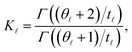 | (14) |
which can be found by imposing (i) that
q(
x) is normalized to 1 (
i.e.,

) and (ii) that the first moment is the only scaling length (
i.e.,
).
2. The distribution, p〈Ntree〉(n), of branch sizes n. For 1 ≪n ≪ 〈Ntree〉, data from different trees are expected to superimpose and to display universal power-law behavior
| | | p〈Ntree〉(n) ∼ n−(2−ε). | (15) |
3. The distribution p〈Ntree〉(|〈L〉) of end-to-end spatial distances of paths of length = 〈L〉 on trees of mass 〈Ntree〉. The data superimpose, when expressed as functions of the scaled distances,  :
:
| | 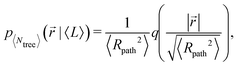 | (16) |
and the function
q =
q(
x) is expected to be of the following RdC form:
| | | q(x) = Cpathxθpathexp(−(Kpathx)tpath). | (17) |
4. The distribution p〈Ntree〉() of vector distances between tree nodes. Once again, data from different 〈Ntree〉 are expected to superimpose when expressed as functions of the scaled distances,  :
:
| |  | (18) |
and, again, the function
q =
q(
x) is expected to be of the RdC form,
| | | q(x) = Ctreexθtreeexp(−(Ktreex)ttree). | (19) |
The two sets of exponents (
θpath,
tpath) (
eqn (17)) and (
θtree,
ttree) (
eqn (19)) depend on the tree universality class, while the two sets of numerical factors (
Cpath,
Kpath) and (
Ctree,
Ktree) are given by the analytical expressions,
| | 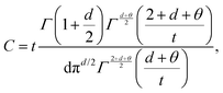 | (20) |
| |  | (21) |
obtained by imposing (i) that
q(
x) is normalized to 1 (
i.e.,

) and (ii) that the second moment is the only scaling length (
i.e.,
).
Notice that general scaling arguments34 imply the following fundamental relations between the exponents of RdC functions and the exponents characterizing observables: θ = 1/ρ − 1, t = 1/(1 − ρ), tpath = 1/(1 − νpath), θtree = min(θpath, 0), ttree = 1/(1 − ν). The only independent exponent is θpath, which turns out to be >0 based on numerical estimates. Accordingly, θtree = 0. For a detailed characterization of lattice trees in terms of distribution functions and how these are related to RdC functions and their exponents, the reader is referred to ref. 34.
3.2.2 Extrapolation of exponents from data for finite-size trees.
For each 〈Ntree〉, estimates of exponents and corresponding errors (θ ± Δθ, t ± Δt), (θpath ± Δθpath, tpath ± Δtpath) and (θtree ± Δθtree, ttree ± Δttree) were obtained by best fit of RdC functions eqn (12) (with eqn (13) and (14)), eqn (17) and (19) (with eqn (20) and (21)) to, respectively, data sets for p〈Ntree〉(), p〈Ntree〉(|〈L〉) and p〈Ntree〉(). Results are collected in Table S4 in SI.
Then, to extrapolate the values and errors in the asymptotic regime 〈Ntree〉 → ∞, we have fitted the straight line
to the data (1/〈
Ntree〉,
θ), and so on for the other exponents, for the three largest 〈
Ntree〉's and with fit parameters
A and
B (see Fig. S4 in SI for a graphical illustration of the procedure). The intercept with the
y-axis,
B, gives the extrapolated value, while error estimate of the extrapolated value is obtained by repeating this procedure to data sets (1/〈
Ntree〉,
θ + Δ
t) and (1/〈
Ntree〉,
θ − Δ
t) and so on for the other exponents. Final results are summarized in
Table 2. For comparison, we report also the measured values of the exponents for 2d tree melts published originally in
ref. 34.
Table 2 Exponents characterizing the Redner-des Cloizeaux behavior of distribution functions (column 1) and relations to other exponents (column 2, see ref. 34 for details). Column 3 reports the values for 2d tree melts estimated in ref. 34. Columns 4 to 6 report the estimated values for the tree-like primitive shapes of the 2d ring melts considered in this work, for different ring bending stiffness κbend. For technical details on the derivation of these exponents, see Section 3.2.2
|
|
Relation to other exponents34 |
Measured value (ref. 34) |
Measured value (this work) |
|
κ
bend = 0 |
κ
bend = 1 |
κ
bend = 1.5 |
|
θ
|

|
0.593 ± 0.003 |
0.421 ± 0.001 |
0.430 ± 0.002 |
0.413 ± 0.003 |
|
t
|

|
2.35 ± 0.01 |
2.631 ± 0.006 |
2.605 ± 0.009 |
2.57 ± 0.01 |
|
θ
path
|
— |
0.63 ± 0.04 |
0.679 ± 0.001 |
0.711 ± 0.002 |
0.6602 ± 0.0004 |
|
t
path
|

|
4.2 ± 0.1 |
6.132 ± 0.006 |
4.665 ± 0.003 |
2.94 ± 0.02 |
|
θ
tree
|
min(θpath, 0) = 0 |
−0.14 ± 0.02 |
−0.09 ± 0.009 |
−0.07 ± 0.01 |
−0.06 ± 0.01 |
|
t
tree
|

|
1.857 ± 0.005 |
1.75 ± 0.02 |
1.72 ± 0.03 |
1.65 ± 0.02 |
4 Results
4.1 Observables
We start first with the mean path length 〈L〉 as a function of the mean tree weight 〈Ntree〉 (eqn (4)), and determine the exponent ρ by using the methods of Section 3.1.2. The results for 〈L〉 vs. 〈Ntree〉 for different κbend parameters are shown in panel (a) of Fig. 4 (symbols) together with the estimated values and statistical errors for ρ (dashed lines). In particular, the behavior is in very good agreement with the results for 2d tree melts33 (Table 1). Interestingly, by introducing the asymptotic (i.e., large-〈Ntree〉) fraction of branch-nodes Λ (see r.h.s. panel of Fig. S3 in SI), its inverse Λ−1 corresponds to the mean path length between two branch-nodes47 and, so, to the natural length scale beyond which branching becomes effectively relevant. As a consequence, data for individual κbend collapse onto a single master curve (Fig. 4(a), inset) by rescaling the x- and y-coordinate as the following:| |  | (23) |
| |  | (24) |
where ρ = 0.61 in eqn (24) is the average¶ of the estimated best values for individual κbend (Table 1).
 |
| | Fig. 4 Conformational properties of trees: observables (symbols) and asymptotic power-law behaviors (dashed lines). (a) 〈L〉 ∼ 〈Ntree〉ρ, mean path length as a function of the mean tree weight 〈Ntree〉. (b) 〈Nbr〉 ∼ 〈Ntree〉ε, mean branch weight as a function of the mean tree weight 〈Ntree〉. (c) 〈Rpath2〉 ∼ 〈L〉2νpath, mean-square end-to-end spatial distance of paths of length = 〈L〉. (d) 〈Rg2〉 ∼ 〈Ntree〉2ν, mean-square gyration radius as a function of the mean tree weight 〈Ntree〉. In each panel the dashed lines express the interval of possible values for the exponent, lying between the minimum lower-bound and the maximum upper-bound for all κbend (see Table 1). (Inset) Universal scaling plots for the observables. Here, the value of the exponent used in each plot corresponds to the average of the estimated best values for individual κbend (see Table 1). | |
Then, we consider the mean branch weight 〈Nbr〉 as a function of 〈Ntree〉 (eqn (5)), and determine the related exponent ε, see panel (b) of Fig. 4 (symbols and dashed lines). As before, our estimates for ε for individual κbend are in agreement with each other and with the corresponding measured values for 2d tree melts33 (Table 1); moreover, it is important to emphasize that our estimated values satisfy also the relation ε = ρ with great accuracy. Finally, data for individual κbend collapse onto a single master curve (Fig. 4(b), inset) by rescaling the x-coordinate according to eqn (23) and, analogously to eqn (24), the y-coordinate as the following:
| |  | (25) |
where
ε = 0.63 in
eqn (25) is the average of the estimated best values for individual
κbend (
Table 1).
Third, we consider the mean-square end-to-end spatial distance 〈Rpath2〉 as a function of the mean path length 〈L〉 (eqn (6)), and determine the related exponent νpath, see panel (c) of Fig. 4 (symbols and dashed lines). Similarly to previous results, the estimated νpath for κbend = 0 and κbend = 1 agree well with each other and with the measured value for 2d tree melt (Table 1); instead, the estimated value for κbend = 1.5 now is ≈13% smaller. We argue that this discrepancy may be due to the limited amount of branching observed for κbend = 1.5 compared to the structures in the other two cases (r.h.s. panel of Fig. S3 in SI): in fact, for Λ → 0 one recovers the linear chain limit where νpath = ν = 1/2. At the same time, the reported difference between the value of νpath for κbend = 1.5 and the other values is not large, so we decide to ignore it in the rest of the discussion and proceed with the analysis in the same manner as we did for the other observables. In this regard, we notice that data for individual κbend are already on top of each other. Nonetheless, it is useful to rescale the x- and y-coordinates as the following:
| |  | (26) |
| | | 〈Rpath2〉 → 〈Rpath2〉〈L〉−2νpath, | (27) |
where
νpath = 0.75 in
eqn (27) is the average of the estimated best values for individual
κbend (
Table 1). The result (see inset of
Fig. 4(c)) confirms the universal behavior and suggests that the mean-square end-to-end distance between two branch-nodes is ≃(1/
Λ)
2νpath.
To conclude, we examine the mean-square gyration radius 〈Rg2〉 as a function of 〈Ntree〉 (eqn (7)), and determine the related exponent ν, see panel (d) of Fig. 4 (symbols and dashed lines). Also in this last case, the estimated ν for κbend = 0 and κbend = 1 agree well with each other and with the measured value for 2d tree melt (Table 1); again the estimated value for κbend = 1.5 is slightly (≈8%) smaller, but we disregard this small difference in the analysis. Overall, we confirm the general scaling relation ν = ρνpath relating the different exponents. Finally, based on the results for the previous observables, we expect data for individual κbend to collapse on top of each other assuming eqn (23) for the rescaling of the x-coordinate and
| |  | (28) |
for the
y-coordinate, and where
ν = 0.49 in
eqn (28) is the average of the estimated best values for individual
κbend (
Table 1). The plot in the inset of
Fig. 4(d) confirms our scaling ansatz.
To summarize this first part, the analysis of the primitive shapes of ring polymers in 2d melt by means of the same fundamental observables used to study melts of randomly branching polymers has shown that these latter systems are fundamentally analogous to the former. In the next Section, we generalize the analysis to the distribution functions.
4.2 Distribution functions
We start with the path length distribution functions, p〈Ntree〉(). As illustrated in Fig. 5, the measured p〈Ntree〉() for different tree sizes fall onto universal master curves, when plotted as a function of the rescaled path length x = /〈L〉 (eqn (11)), which are well described by the RdC form eqn (12)–(14) (dashed lines). Noticeably, the estimated values of the asymptotic exponents (θ, t) (see Section 3.2.2 for details) for the different chain flexibilities κbend are in good agreement with each other and relatively close to the measured values34 for trees in 2d melts (see Table 2).
 |
| | Fig. 5 Conformational properties of trees: p〈Ntree〉(), distribution functions of linear paths of length . The dashed line of each panel corresponds to the predicted RdC functional form for trees, eqn (12)–(21), with the exponents θ and t as in Table 2. Data of different colors denote different mean tree weight 〈Ntree〉 (see legend). | |
Next, we consider the distribution functions of branch weight n, p〈Ntree〉(n). Data for different tree sizes 〈Ntree〉 are in very good agreement (Fig. 6) with the predicted (eqn (15)) power-law behavior p〈Ntree〉(n) ∼ n−(2−ε) for trees (dashed lines, ε is as in panel (b) of Fig. 4).
 |
| | Fig. 6 Conformational properties of trees: p〈Ntree〉(n), distribution functions of branch weight n. The dashed lines express the interval of possible values for the exponent ε (see Fig. 4(b)), lying between the minimum lower-bound and the maximum upper-bound for all κbend (see Table 1). Colorcode/symbols are as in Fig. 5. | |
Then, we consider the distribution functions p〈Ntree〉(|〈L〉) of end-to-end spatial distances of linear paths of length =〈L〉. When plotted as a function of the rescaled distance,  , the measured curves for different κbend fall onto single universal master curves (Fig. 7). Here, however, and contrarily to the results presented so far, the master curves for the different stiffnesses agree less well with each other. This, in particular, can be seen by the fact that the asymptotic RdC ansatz (dashed lines) are characterized by quite distinct values for the exponents θpath and, especially, tpath (see Table 2).
 |
| | Fig. 7 Conformational properties of trees: p〈Ntree〉(|〈L〉), distribution functions of end-to-end spatial distances of paths of length =〈L〉. The dashed line of each panel corresponds to the RdC functional form for trees, eqn (17) with eqn (20) and (21), with the exponents θpath and tpath as in Table 2. Colorcode/symbols are as in Fig. 5. | |
Finally, we consider the distribution functions p〈Ntree〉() of vector distances between tree nodes. By rescaling the x-axis by the square-root of the corresponding momenta  curves from different rings obey universal behavior (Fig. 8). This behavior is well described (dashed lines) by the RdC function eqn (19), with estimated values for the exponents θtree and ttree for the different flexibilities κbend in good agreement with each other and close to the estimated values for 2d tree melts (Table 2).
 |
| | Fig. 8 Conformational properties of trees: p〈Ntree〉(), distribution functions of vector distances between tree nodes. The dashed line of each panel corresponds to the RdC functional form for trees, eqn (19) with eqn (20) and (21), with the exponents θtree and ttree as in Table 2. Colorcode/symbols are as in Fig. 5. | |
In conclusion, the results for both observables and distribution functions which have been presented so far demonstrate (besides some discrepancies detected in the distribution functions p〈Ntree〉(|〈L〉) for node-to-node spatial distances of linear paths) that the tree-like primitive paths of ring polymers in 2d melts obey the same statistics of 2d melts of randomly branching polymers. We now explore the connection between these two systems in relation to polymer dynamics.
5 A note on ring dynamics
Although it is not the main purpose of this work, we present here a few results on ring dynamics as well. In fact, as originally pointed out by Rubinstein and coworkers8,10 and reaffirmed at various degrees of sophistications in later works,16,48–50 fingerprints of the tree-like structure of rings in melt can be found in ring dynamics.
In particular, in ref. 16 it was suggested that the relaxation time of the chains as a function of the monomers number Nring is given by the power-law behavior
| | | τrelax = τmicrN2+(1−θ)ρ+θνring, | (29) |
where
τmicr is a “microscopic” time scale of the order of the time needed for the chain to relax between pairs of neighboring topological obstacles. The
ρ and
ν exponents in
eqn (29) are the same describing the behaviors of observables 〈
L〉 (
eqn (4)) and 〈
Rg2〉 (
eqn (7)) as functions of
Nring, while the parameter 0 ≤
θ ≤ 1 (not to be confused with the various exponents
θ associated to the RdC functions) quantifies the postulated phenomenon of so called tube dilation: in analogy to linear chains,
40,41 the array of topological obstacles where ring polymers relax can be assimilated to the relaxation inside a tube-like region shaped by the same obstacles. Assuming such obstacles as fixed,
48 the tube is a static structure and
θ = 0;
vice versa,
16 assuming that chain relaxation proceeds self-similarly at all scales (as in ordinary Rouse model
40), the tube “dilate” with time and
θ = 1. As shown in
ref. 16,
eqn (29) applies well to the case of melt of rings in 3d with
θ = 1,
i.e. in good agreement with the mechanism of complete tube dilation. What about the case of 2d melts, which we should expect to be very different from the 3d case because different chains can not, for instance, thread each other?
To answer this question, we have computed τrelax for our rings by defining it as the time scale for the entire ring to diffuse a distance equal to its mean-size, i.e.
| | | g3(t = τrelax) = 〈Rg2〉ring, | (30) |
where
| | | g3(t) ≡ 〈(cm(t) − cm(0))2〉 | (31) |
is the mean-square displacement of the chain centre of mass. Results for
τrelax, normalized by
Nring2, as a function of
Nring are shown in the top panel of
Fig. 9. Interestingly the data suggest the scaling
τrelax ∼
Nring2, therefore they are not compatible with the power-law
(29) whose exponent is, by construction, strictly >2. To validate this result further, we consider the scaling behavior of the chain diffusion coefficient,
| |  | (32) |
for which we expect
Dring ∼ 〈
Rg2〉/
τring ∼
N−2(1−ν)ring =
Nring−1. We have estimated diffusion coefficients by best fits of data for
g3(
t) to a simple linear function (
eqn (32)), with the fit procedure restricted to the time interval
t > 5
τrelax (see Fig. S5 in SI). Results for
Dring, each multiplied by the corresponding
Nring, are shown in the bottom panel of
Fig. 9 for each stiffness
κbend, and they confirm the scaling analysis.
 |
| | Fig. 9 Ring dynamics: (top) Ring relaxation time normalized by the square ring monomer number, τrelax/Nring2, as a function of Nring. (bottom) Ring diffusion coefficient normalized by the inverse ring monomer number, Dring/Nring−1, as a function of Nring. Colorcode/symbols are for different chain stiffness κbend (see legend, as in Fig. 4). Dotted lines joining the symbols serve as a guide for the eye. Upraising of the data for Nring = 1280 is due to the limited length of the MC trajectory (see Fig. S5 in SI). | |
Curiously, we notice that the power-law behaviors τrelax ∼ Nring2 and Dring ∼ Nring−1 reported here are the same that one would have expected for an ordinary Rouse chain in ideal (i.e., no volume interactions) conditions.40,41 For the polymers considered here this is obviously not the case, and the agreement with the Rouse model must be considered a fortuituous coincidence for which, at the moment, we have no physical intuition. We just conclude by highlighting the fact that the two power-laws are no artefact of the present lattice model, as they were also reported in previous molecular simulations of 2d ring melts.51
6 Summary and conclusions
In this work we have performed a detailed analysis of the conformational properties of unknotted and non-concatenated ring polymers in 2d melt conditions (Fig. 3), aiming at demonstrating that rings double-fold around randomly branching (tree-like) conformations as originally proposed by Khokhlov, Nechaev, Rubinstein and others.7,8,10 In particular, after reconstructing the “primitive shapes” of ring conformations from Monte Carlo computer simulations of a generic polymer model on the two-dimensional triangular lattice, we proceeded with an analysis of said branched structures by means of the same observables and distribution functions (Section 3) used for the analysis of lattice trees.
We thus confirm (Section 4, in particular Fig. 4–8) that the conformational properties of the branched structures are, in general, in good agreement with the measured properties33,34 of two-dimensional branched polymers in melt conditions. At the same time, a closer look reveals also interesting quantitative differences: for instance, some of the exponents which characterize the distribution functions (for instance tpath, see Table 2) show larger discrepancies between themselves and the corresponding predicted values for trees than the exponents for observables (Table 1). We argue that these deviations from tree behavior emerge because our rings are not perfectly double-folded52 around their “primitive shape” (see Section 2.3), and then the “mapping” between rings and trees works only approximately. In this regard, it is worth remarking that the analysis of ring dynamics (Section 5) also suggests a rather different behavior than the one expected based on the branched shapes of the rings. In fact, the rings' relaxation time is found to be faster than the theoretical predictions, scaling “only” quadratically with the rings' mass and, therefore, surprisingly close to the result expected for ordinary Rouse motion.
We conclude with an outlook for future work. Besides trying to understand the origin of the reported deviations between rings and the tree description, it would be even more interesting (and challenging) to generalize the analysis of this work to three-dimensional melts of rings. As a matter of fact, how rings fold in 3d is still not fully understood. In fact, while on one side a multi-scale numerical protocol based on the random-tree model29 reveals an accurate similarity between some of the trees' and rings' static properties, on the other the “tree picture” cannot be considered complete since, for example, one of two nearby rings may easily penetrate onto an open loop of the other without violation of topological constraints. Although rare, such so-called threading events30,31,53–55 have been observed and are thought to be responsible of some exotic properties in rings' out-of-equilibrium behavior.56–60 For these reasons, developing an algorithm for the reconstruction of the chain's “primitive shape” along the lines of Section 2.3 would represent an important contribution towards the comprehension of these fundamental systems.
Author contributions
MAU and AR contributed equally to this work.
Conflicts of interest
There are no conflicts to declare.
Data availability
The data supporting this article are included in the supplementary information (SI). Supplementary information provides: the data supporting this article and some complementing figures. See DOI: https://doi.org/10.1039/d5sm00947b.
Acknowledgements
MAU is supported by an EMBO Postdoctoral Fellowship (ALTF 1305-2024). AR acknowledges S. K. Nechaev for insightful discussions, and financial support from PNRR Grant CN_00000013_CN-HPC, M4C2I1.4, spoke 7, funded by Next Generation EU.
References
- S. F. Edwards, Proc. Phys. Soc., 1967, 92, 9–16 CrossRef CAS.
- P. G. de Gennes, J. Chem. Phys., 1971, 55, 572–579 CrossRef.
- R. Everaers, S. K. Sukumaran, G. S. Grest, C. Svaneborg, A. Sivasubramanian and K. Kremer, Science, 2004, 303, 823 CrossRef CAS PubMed.
- D. J. Read, K. Jagannathan and A. E. Likhtman, Macromolecules, 2008, 41, 6843–6853 CrossRef CAS.
- N. Uchida, G. S. Grest and R. Everaers, J. Chem. Phys., 2008, 128, 044902 CrossRef PubMed.
- R. Everaers, H. A. Karimi-Varzaneh, F. Fleck, N. Hojdis and C. Svaneborg, Macromolecules, 2020, 53, 1901–1916 CrossRef CAS.
- A. R. Khokhlov and S. K. Nechaev, Phys. Lett. A, 1985, 112, 156–160 CrossRef.
- M. Rubinstein, Phys. Rev. Lett., 1986, 57, 3023–3026 CrossRef CAS PubMed.
- S. K. Nechaev, A. N. Semenov and M. K. Koleva, Phys. A, 1987, 140, 506–520 CrossRef.
- S. P. Obukhov, M. Rubinstein and T. Duke, Phys. Rev. Lett., 1994, 73, 1263–1266 CrossRef CAS PubMed.
- M. G. Brereton and T. A. Vilgis, J. Phys. A: Math. Gen., 1995, 28, 1149–1167 CrossRef CAS.
- A. L. Kholodenko and T. A. Vilgis, Phys. Rep., 1998, 298, 251–370 CrossRef CAS.
- T. Sakaue, Phys. Rev. Lett., 2011, 106, 167802 CrossRef PubMed.
- S. Obukhov, A. Johner, J. Baschnagel, H. Meyer and J. P. Wittmer, EPL, 2014, 105, 48005 CrossRef.
- A. Y. Grosberg, Soft Matter, 2014, 10, 560–565 RSC.
- T. Ge, S. Panyukov and M. Rubinstein, Macromolecules, 2016, 49, 708–722 CrossRef CAS PubMed.
- F. Ferrari, J. Paturej, M. Piatek and Y. Zhao, Nucl. Phys. B, 2019, 945, 114673 CrossRef CAS.
- M. Kapnistos, M. Lang, D. Vlassopoulos, W. Pyckhout-Hintzen, D. Richter, D. Cho, T. Chang and M. Rubinstein, Nat. Mater., 2008, 7, 997–1002 CrossRef CAS PubMed.
- R. Pasquino, T. C. Vasilakopoulos, Y. C. Jeong, H. Lee, S. Rogers, G. Sakellariou, J. Allgaier, A. Takano, A. R. Brás, T. Chang, S. Gooßen, W. Pyckhout-Hintzen, A. Wischnewski, N. Hadjichristidis, D. Richter, M. Rubinstein and D. Vlassopoulos, ACS Macro Lett., 2013, 2, 874–878 CrossRef CAS PubMed.
- M. Kruteva, J. Allgaier and D. Richter, Macromolecules, 2017, 50, 9482–9493 CrossRef CAS.
- M. Kruteva, J. Allgaier, M. Monkenbusch, L. Porcar and D. Richter, ACS Macro Lett., 2020, 9, 507–511 CrossRef CAS PubMed.
- M. Kruteva, M. Monkenbusch, J. Allgaier, O. Holderer, S. Pasini, I. Hoffmann and D. Richter, Phys. Rev. Lett., 2020, 125, 238004 CrossRef CAS PubMed.
- M. Kruteva, J. Allgaier and D. Richter, Macromolecules, 2023, 56, 7203–7229 CrossRef CAS.
- M. E. Cates and J. M. Deutsch, J. Phys. France, 1986, 47, 2121–2128 CrossRef CAS.
- M. Müller, J. P. Wittmer and M. E. Cates, Phys. Rev. E: Stat. Phys., Plasmas, Fluids, Relat. Interdiscip. Top., 1996, 53, 5063–5074 CrossRef PubMed.
- M. Müller, J. P. Wittmer and M. E. Cates, Phys. Rev. E: Stat. Phys., Plasmas, Fluids, Relat. Interdiscip. Top., 2000, 61, 4078–4089 CrossRef PubMed.
- J. D. Halverson, W. B. Lee, G. S. Grest, A. Y. Grosberg and K. Kremer, J. Chem. Phys., 2011, 134, 204904 CrossRef PubMed.
- J. D. Halverson, W. B. Lee, G. S. Grest, A. Y. Grosberg and K. Kremer, J. Chem. Phys., 2011, 134, 204905 CrossRef PubMed.
- A. Rosa and R. Everaers, Phys. Rev. Lett., 2014, 112, 118302 CrossRef PubMed.
- R. D. Schram, A. Rosa and R. Everaers, Soft Matter, 2019, 15, 2418–2429 RSC.
- M. A. Ubertini, J. Smrek and A. Rosa, Macromolecules, 2022, 55, 10723–10736 CrossRef CAS PubMed.
- A. Rosa and R. Everaers, J. Phys. A: Math. Theor., 2016, 49, 345001 CrossRef.
- A. Rosa and R. Everaers, J. Chem. Phys., 2016, 145, 164906 CrossRef PubMed.
- A. Rosa and R. Everaers, Phys. Rev. E, 2017, 95, 012117 CrossRef PubMed.
- V. Hugouvieux, M. A. V. Axelos and M. Kolb, Macromolecules, 2009, 42, 392–400 CrossRef CAS.
- R. D. Schram and G. T. Barkema, J. Comput. Phys., 2018, 363, 128–139 CrossRef CAS.
- M. A. Ubertini and A. Rosa, Phys. Rev. E, 2021, 104, 054503 CrossRef CAS PubMed.
- M. Rubinstein, Phys. Rev. Lett., 1987, 59, 1946–1949 CrossRef CAS PubMed.
- N. Metropolis, A. W. Rosenbluth, M. N. Rosenbluth, A. H. Teller and E. Teller, J. Chem. Phys., 1953, 21, 1087–1092 CrossRef CAS.
-
M. Doi and S. F. Edwards, The Theory of Polymer Dynamics, Clarendon, Oxford, 1986 Search PubMed.
-
M. Rubinstein and R. H. Colby, Polymer Physics, Oxford University Press, New York, 2003 Search PubMed.
- K. Kremer and G. S. Grest, J. Chem. Phys., 1990, 92, 5057–5086 CrossRef CAS.
- P. H. W. van der Hoek, A. Rosa and R. Everaers, Phys. Rev. E, 2024, 110, 045312 CrossRef CAS PubMed.
- E. J. Janse van Rensburg and N. Madras, J. Phys. A: Math. Gen., 1992, 25, 303–333 CrossRef.
- S. Redner, J. Phys. A: Math. Gen., 1980, 13, 3525–3541 CrossRef CAS.
-
J. des Cloizeaux and G. Jannink, Polymers in Solution, Oxford University Press, Oxford, 1989 Search PubMed.
- M. Daoud and J. F. Joanny, J. Phys. France, 1981, 42, 1359–1371 CrossRef CAS.
- J. Smrek and A. Y. Grosberg, J. Phys.: Condens. Matter, 2015, 27, 064117 CrossRef CAS PubMed.
- E. Ghobadpour, M. Kolb, M. R. Ejtehadi and R. Everaers, Phys. Rev. E, 2021, 104, 014501 CrossRef CAS PubMed.
- E. Ghobadpour, M. Kolb, I. Junier and R. Everaers, Macromolecules, 2025, 58, 10632–10646 CrossRef CAS.
- J. Kim, J. M. Kim and C. Baig, Soft Matter, 2021, 17, 10703–10715 RSC.
- A. Rosa and R. Everaers, Eur. Phys. J. E: Soft Matter Biol. Phys., 2019, 42, 1–12 CrossRef CAS PubMed.
- D. Michieletto, Soft Matter, 2016, 12, 9485–9500 RSC.
- J. Smrek and A. Y. Grosberg, ACS Macro Lett., 2016, 5, 750–754 CrossRef CAS PubMed.
- J. Smrek, K. Kremer and A. Rosa, ACS Macro Lett., 2019, 8, 155–160 CrossRef CAS PubMed.
- D. Michieletto and M. S. Turner, Proc. Natl. Acad. Sci. U. S. A., 2016, 113, 5195–5200 CrossRef CAS PubMed.
- Q. Huang, J. Ahn, D. Parisi, T. Chang, O. Hassager, S. Panyukov, M. Rubinstein and D. Vlassopoulos, Phys. Rev. Lett., 2019, 122, 208001 CrossRef CAS PubMed.
- T. C. O'Connor, T. Ge, M. Rubinstein and G. S. Grest, Phys. Rev. Lett., 2020, 124, 027801 CrossRef PubMed.
- J. Smrek, I. Chubak, C. N. Likos and K. Kremer, Nat. Commun., 2020, 11, 26 CrossRef CAS PubMed.
- C. Micheletti, I. Chubak, E. Orlandini and J. Smrek, ACS Macro Lett., 2024, 13, 124–129 CrossRef CAS PubMed.
Footnotes |
| † For ring polymers, it is implicitly assumed the periodic boundary condition along the chain N + 1 ≡ 1. |
| ‡ As noticed in works,32–34,43 there is no substantial loss of generality by choosing a model for branched polymers where nodes host no more than three bonds compared to models featuring nodes with more than three bonds protruding from them. |
| § In the mentioned works32,33Ntree is not a fluctuating quantity. Here, as shown in the l.h.s. panel of Fig. S3 in SI, the relative fluctuations around the mean value 〈Ntree〉 become rapidly small in the large-Nring limit, so they are expected to have a negligible effect on the estimation of scaling exponents. |
| ¶ The excellent collapse in the inset of Fig. 4(a) and the agreement between the measured ρ-values for individual κbend justifies a posteriori our choice for taking the average. In the rest of this work, we do the same also for the other exponents. |
|
| This journal is © The Royal Society of Chemistry 2025 |
Click here to see how this site uses Cookies. View our privacy policy here. 
 a and
Angelo
Rosa
a and
Angelo
Rosa


 has been fixed based on the monomer number density
  that guarantees melt conditions. All these systems have been studied for bending stiffness parameters κbend = 0, 1, 1.5 (eqn (1)). For completeness, we report the measured MC acceptance rate as a function of the chain stiffness: 0.125 (κbend = 0), 0.021 (κbend = 1), 0.018 (κbend = 1.5). Notice that they are in line with the reported31 acceptance rates for 3d ring melts.

 . Asymptotically, g2(t→∞) = 2〈Rg2〉ring where
 . For each ring in a typical melt configuration (panel (b) of Fig. 3), we identified first the honeycomb lattice sites residing within its contour which allow us to identify, without ambiguity, the nodes of the associated “backbone”. Then, we connect any two of these nodes of the honeycomb lattice by an edge whenever they are spatial nearest neighbors. Visual inspection on the obtained conformations (black lines in panel (c) of Fig. 3) confirms indeed a pronounced tree-like architecture.
 where the corresponding trees reside. (b) Snapshots of ring melt configurations for Nring = 1280 and κbend = 0, 1, 1.5 (from left to right, see legend). (c) Examples of single ring polymers (blue/green/red circular contours) isolated from their corresponding melts, along with their primitive tree-like backbones (black lines inside each circular contour). Notice that the trees contain a certain amount of loops. (d) Final, loop-less, primitive shapes obtained by randomly removing one bond in each of the former loops. Shown on the l.h.s. of the figure, zoomed-in selected portions of tree conformations for κbend = 0 with loops and without loops after bonds removal.
 and
and  and
and  is the spatial position of the tree center of mass.


 ) and (ii) that the first moment is the only scaling length (i.e.,
  ).
).
 :
:
 :
:


 ) and (ii) that the second moment is the only scaling length (i.e.,
  ).
).


 , the measured curves for different κbend fall onto single universal master curves (Fig. 7). Here, however, and contrarily to the results presented so far, the master curves for the different stiffnesses agree less well with each other. This, in particular, can be seen by the fact that the asymptotic RdC ansatz (dashed lines) are characterized by quite distinct values for the exponents θpath and, especially, tpath (see Table 2).
 curves from different rings obey universal behavior (Fig. 8). This behavior is well described (dashed lines) by the RdC function eqn (19), with estimated values for the exponents θtree and ttree for the different flexibilities κbend in good agreement with each other and close to the estimated values for 2d tree melts (Table 2).

