
 Open Access Article
 This Open Access Article is licensed under a
 Creative Commons Attribution 3.0 Unported Licence
Equilibrium phases and phase transitions in multicritical magnetic polymers
Alberto
Raiola
 ab,
Emanuele
Locatelli
ab,
Davide
Marenduzzo
*c and
Enzo
Orlandini
ab
ab,
Emanuele
Locatelli
ab,
Davide
Marenduzzo
*c and
Enzo
Orlandini
ab
aDipartimento di Fisica e Astronomia, Università di Padova, Via Marzolo 8, I-35131 Padova, Italy
bINFN, Sezione di Padova, Via Marzolo 8, I-35131 Padova, Italy
cSUPA, School of Physics and Astronomy, University of Edinburgh, Peter Guthrie Tait Road, Edinburgh EH9 3FD, UK. E-mail: davide.marenduzzo@ed.ac.uk
First published on 22nd May 2025
Abstract
Magnetic polymers are examples of composite soft materials in which the competition between the large configurational entropy of the soft substrate (polymer) and the magnetic interaction may give rise to rich equilibrium phase diagrams as well as non-standard critical phenomena. Here, we study a self-avoiding walk model decorated by Ising spins of value 0 and ±1 that interact according to a Blume–Emery–Griffith-like Hamiltonian. By using mean-field approximations and Monte Carlo simulations, we report the existence of three distinct equilibrium phases: swollen disordered, compact ordered, and compact disordered. Notably, these phases are separated by phase boundaries that meet at multicritical points, whose nature and location are tunable and depend on the strength of the interactions. In our conclusion, we discuss the relevance of the phase diagrams we have obtained to the physics of magnetic polymers and their application to chromatin biophysics.
I. Introduction
Models of magnetic polymers, where each monomer carries a magnetic moment or spin, are an interesting class of interacting systems that have recently received much attention in polymer physics, biophysics, and statistical mechanics. There are multiple reasons for this. First, the flexibility of the polymeric substrate and its relatively low density are important features to exploit in organic magnetic materials with technological applications in, for instance, communication and information.1–3 Second, from the statistical mechanics perspective, they are examples of interacting systems where the spatial organisation (entropy) of the polymer chain and the magnetic interactions between spins may give rise to several conformational phases and phase transitions.4–8 Finally, in the last few years, models of magnetic polymers have been successfully exploited to understand how the interplay between the chromatin folding in 3D and the epigenetic landscape in 1D, regulated by histone marks, can contribute to shaping the genome organization in the nucleus.9,10A precursor of these models, introduced in ref. 4, described the polymer as a self-avoiding walk (SAW) on a hypercubic lattice whose monomers are decorated by Ising spin variables σi = ±1; the monomers interact via the standard ferromagnetic Ising Hamiltonian among themselves, when they are nearest neighbours in 3D space, and with an external magnetic field h. By performing both a mean-field analysis and Monte Carlo simulations of the 3D system (the SAW on the cubic lattice) it was shown that, by increasing the ferromagnetic coupling, this model displays, at h = 0, a first-order phase transition between a swollen and paramagnetic (disordered) phase (SD) and a compact ferromagnetic (ordered) phase (CO). The first-order character is a notable feature of this magnetic model, since in a standard (i.e., non-magnetic) polymer collapse the (Θ) phase transition is known to be second order.11 Later studies have either focused on better determining the location and nature of the transition in two and three dimensions by numerical simulations and finite-size scaling,5,7 or studied the emergence of a ferromagnetic phase transition as a function of the fractal dimension of the polymer substrate.6
Recently, a model of magnetic polymers with 3-state variables (qi = 1, −1, 0) each representing an epigenetic mark, has been introduced to describe the interplay between the 3D organisation of the eukaryotic genome and the 1D epigenetic profile of biochemical marks on chromatin (the DNA-histone composite polymer which provides the building block of chromosomes in eukaryotes).9 Analytical calculations based on mean-field approximation and molecular dynamics simulations have shown that a first-order phase transition rules both the spreading of a single epigenetic mark and the folding of the chromosome into a compact structure. The first-order nature of the transition is important, as it endows the system with memory, which allows a cell to “remember” its state following cell division.10
Note that, similarly to the works cited above, this biophysical model can display only two equilibrium phases: a swollen disordered (SD) phase and a compact (magnetically) ordered (CO) phase. To observe a third phase corresponding to a compact chromatin phase where the epigenetic marks (spins) are incoherently distributed, as in gene deserts regions observed in Drosophila,12 an extension to a non-equilibrium system was needed.13
An interesting problem that emerges from the previous studies is whether there exist spin models embedded in fluctuating filaments that can sustain more than two phases (SD and CO) and multiple phase transitions at equilibrium. A first attempt to investigate this issue was made very recently in ref. 14 where, by introducing an energy offset εoff in the interaction energy of a polymer Potts model, a compact disordered (CD) phase was obtained above a critical value of εoff.
In this paper, we study how a model of a magnetic system with a rich phase diagram and multicritical points, once embedded in a polymer chain, can affect the polymer's magnetic and spatial organisation. This investigation is carried out analytically, at the mean-field level, and numerically, by simulating the magnetic polymer on a cubic lattice.
The paper is organized as follows. In Section II we introduce the magnetic polymer model and derive the mean-field free energy density and the relevant order parameters such as the monomer density and the magnetization. In Section III the mean-field conformational/magnetic phase diagram and the nature of the several phase transitions found are determined as a function of the magnetic coupling parameters. Section IV presents the Monte Carlo simulations of a self-avoiding walk model in the cubic lattice and compares the obtained numerical results with the mean-field findings along some relevant lines of the phase diagram. Finally, Section V is devoted to discussions and conclusions.
II. Model and mean-field free energy density
We consider the ensemble of the N-steps self-avoiding walks (SAWs) {γ} on a lattice of coordination number z. By assigning the set {Si} of spin variables Si ∈ {0, ±1} to the lattice sites occupied by a SAW, γ, the Hamiltonian of the system we wish to study is given by | (1) |
The first term in eqn (1) is the standard ferromagnetic interaction with J > 0 being the exchange energy. The interaction is restricted to the pairs (i,j) of nearest neighbor (NN) sites of the lattice occupied by the SAW γ – this is achieved via the adjacency matrix Λγi,j, which is defined as Λγi,j = 1 if i,j are NN on the lattice and Λγi,j = 0 otherwise. The second term, characterized by the parameter K, provides an energy gain for any pair of non-zero NN spins (Si = ±1), irrespective of their sign. Finally, the last term weights the neutral sites on the walk via the dilution parameter Δ (Si = 0). This term introduces a “mitigation” of the ferromagnetic interaction whose amount (i.e., fraction of neutral spins) is ruled by Δ; thus, we can interpret Δ as a chemical potential (Fig. 1). Note that the Hamiltonian eqn (1) was studied by Blume, Emery, and Griffiths (BEG) on a lattice, as a spin-1 model of a diluted uniaxial ferromagnet or of a He3–He4 mixture.15 The key emergent feature of the BEG model is the presence of a tricritical point, separating a line of second-order (continuous) phase transitions from a line of first-order (discontinuous) transitions. In our model, we shall distinguish tricritical points, defined in such a way, from multicritical points, where multiple transition lines (of different order) meet, and triple points, which mark points at which three different phases are in equilibrium.
 | ||
| Fig. 1 Cartoon of a self-avoiding walk on a two-dimensional square lattice. The thick black line represents the polymer backbone, and the thin straight lines represent the underlying lattice. Each node i of the walk holds a spin variable Si which can be equal to −1 (red circle), 0 (white circle), or +1 (blue circle). A dotted line is drawn in correspondence with pairs of spin variables with Si = ±1, which are not nearest neighbors on the walk but in 3D space. | ||
By taking the Boltzmann factor associated to eqn (1) and summing over the spins and the SAW configurations {{Si}, {γ}} we get the partition function of the model:
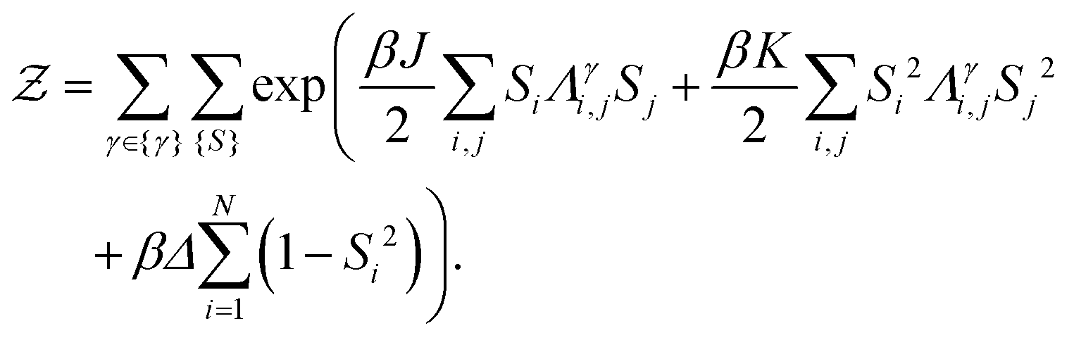 | (2) |
A mean-field estimate for the free energy density corresponding to eqn (2) can be obtained by first decoupling the quadratic and bi-quadratic terms via a double Hubbard–Stratonovich transformation involving two local fields {ϕi} and {αi}, and then performing the sum over the spin degrees of freedom and the SAW configurations (see Appendix A). This procedure gives as a result
 | (3) |
 | (4) |
 | (5) |
 | (6) |
 | (7) |
 | (8) |
III. Mean-field phase diagrams
To analyse the mean-field free energy eqn (3) in the (Δ,T) plane we first divided eqn (7) by eqn (6), obtaining | (9) |
A. The K/J < 1 case
We start from the mean-field phase diagram in the (Δ,T) plane, reported in Fig. 2a, for the case K/J = 0.8, which is representative of the mean-field phase behaviour when K/J < 1. | ||
| Fig. 2 Mean-field results at K/J = 0.8. (a) Equilibrium phase diagram in the (Δ,T) plane: note the emergence of three phases – SD, CO and CD – for Δ < Δ* ≃ −2.04. Dashed (first order) and solid (continuous) lines show the corresponding phase boundaries. The location of the multicritical point (here coinciding with the triple point) (Δ*,T*) ≃ (−2.04,3.05) is highlighted with a red circle. (b) ρ dependence of the free energy density at Δ = Δ*. The thickest red curve marks the case T = T*. (c) and (d) Temperature dependence of the polymer density ρ (c) and the average magnetization per spin m (d) at three different values of Δ. | ||
The first significant feature of note is the presence of three equilibrium phases: (i) a magnetically disordered phase, where the polymer chain is extended (swollen disordered or SD phase); (ii) a compact ordered or CO phase where the polymeric substrate is globular and magnetically ordered (i.e. with most of the spins either up or down); (iii) a magnetically disordered but compact phase (compact disordered or CD phase) where the polymer density is non-zero but the spins are in the paramagnetic phase. The CD phase is especially notable here because it is generally difficult to be observed at equilibrium in simpler models of magnetic polymers.13,14
The phase diagram shows the presence of three phase boundary curves: (i) two first-order phase transition lines, one between the CO and SD phases and the other between the CO and CD phases, and (ii) a second-order (continuous) phase transition between the CD and the SD phase. The three boundaries meet at a multicritical point, at (Δ,T) = (Δ*,T*) (the red circle in Fig. 2a): in the present case of K/J = 0.8, this is also a triple point as the CO, CD and SD phases are all coexisting there.
The nature of the multicritical point is elucidated by the ρ dependence of the free energy density, estimated at Δ = Δ* (see Fig. 2b). For T > T* the absolute minimum of the free energy is at ρ = 0 (swollen phase, SD), while in the region T < T* the global minimum is located at ρ ≈ 0.9 (corresponding to the compact ordered phase, CO); at T = T* (the thickest red curve) two equal height minima are observed, one at ρ = 0 and one at ρ ≃ 0.85. Additionally, as we cross the multicritical point by varying T at fixed Δ = Δ* ≃ −2.04 (see solid lines in Fig. 2c and d), both the m vs. T and the ρ vs. T curves display a finite jump.
Examining the behavior of the curve ρ(T) at different values of Δ clarifies the nature of the transition lines. At Δ = −6 (see the dotted curve in Fig. 2c), upon increasing T, we encounter a discontinuity near the CO/CD boundary; after this jump, the curve gradually decreases, approaching zero as it approaches the CD/SD phase boundary. This suggests a first-order transition at the CO/CD boundary (confirmed by the finite discontinuity in the m vs. T curve, Fig. 2d), followed by a continuous phase transition at the CD/SD boundary.
Finally, the finite discontinuities observed in the m vs. T and ρ vs. T curves at Δ = 4 (see dashed curves in Fig. 2c and d) confirm the first-order nature of the CO/SD phase transition.
B. The K/J > 1 case
When the self-attraction strength exceeds the ferromagnetic interaction, the phenomenology becomes more complex.We start from K/J = 1.8, where the analysis of the corresponding virial coefficients (as shown in Fig. 11c) reveals two key properties of the system: (i) the compact disordered (CD) phase region expands towards higher Δ values, indicating stability at greater dilutions; (ii) as we progress from lower dilution regimes (i.e., from negative Δ values), the nature of the CD/SD phase boundary changes from continuous to first-order. This latter switch coincides with a sign change in the third virial coefficient along this curve, revealing the presence of a tricritical point at Δ* = −2.46 and T* = 6.08. Simultaneously, the triple point shifts to Δtr = 1.95, Ttr = 3.95. In other words, the topology of the phase diagram has fundamentally changed, as the multicritical point at K/J = 0.8 has split into a tricritical and a triple point (see Fig. 3a).
 | ||
| Fig. 3 Mean-field results at K/J = 1.8. (a) Equilibrium phase diagram in the (Δ,T). The SD/CD phase boundary is partitioned into a continuous (solid) and a first-order transition curve (dashed curve). The corresponding tricritical point, located at (Δ*,T*) ≈ (−2.46,6.08) is highlighted by a red circle, while the blue circle marks the triple point (Δtr,Ttr) ≈ (1.95,3.95). (b) Free energy density landscapes at Δ = Δtr = 1.95 as a function of the polymer density ρ. The coexistence of the three phases at the triple point is marked by the three equal height minima at Ttr = 3.95 (thickest line). (c) and (d) Density ρ (c) and magnetization m (d) as functions of T at Δ = −4 (dotted line), Δ = Δtr (solid line) and Δ = 4 (dot-dashed line). | ||
The three-phase coexistence at the triple point can be understood by looking at the ρ dependence of the free energy density computed at Δtr and for some values of T above, below and at Ttr (see Fig. 3b). There are three key points to note. First, for T < Ttr there is a unique absolute minimum located at ρ ≃ 0.88, that corresponds to the CO phase. Second, for T > Ttr the absolute minimum is at ρ = 0, as expected in the swollen phase. Third, at the triple point temperature T = Ttr, the system exhibits three minima of equal depth in its free energy landscape. One of these minima occurs at ρ = 0, while the other two occur at ρ = 0.71 and ρ = 0.88 respectively. This free energy profile describes the coexistence of three distinct phases: two compact (ordered and disordered) and one swollen (disordered). The triple minimum was absent in the lower K/J case, as the transitions between the phases were not all first-order.
This scenario is confirmed in Fig. 3c and d where we report the temperature behavior of ρ and m for Δ = −4.0 and Δtr.
For yet larger values of K/J, the CD phase expands further into the Δ > 0 region and, notably, for K/J ≃ 1.805, the nature of the CO/CD phase boundary splits into a second-order and first-order transition curves that are governed by a novel critical point. Such a phenomenon is evidenced by the analysis of the virial coefficients reported in Fig. 11c and d, which also shows that this crossover is indeed a new, second, tricritical point (Δ**,T**). For K/J ≃ 1.805, such a point is located at Δ** = −∞ and moves to larger values of Δ with increasing K/J. As showcased in the phase diagram of Fig. 4a, for K/J = 2.3 the point is located at Δ** = 0.63, T** = 4.65. The corresponding free energy profile is illustrated by the thickest curve of Fig. 4b and also by the m vs. T and ρ vs. T curves in Fig. 4c and d.
 | ||
| Fig. 4 Mean-field results at K/J = 2.3 (a) equilibrium phase diagram in the (Δ,T) plane. The two red circles highlight the two multicritical points located at (Δ*,T*) = (−3.15,7.76) and (Δ**,T**) = (0.63,4.65). The blue circle locates the triple point (Δtr,Ttr) = (3.98,4.23) (b) free energy profiles for Δ = Δ** = 0.63. The extended flatness of the thicker red line suggests the tricritical nature of the (Δ**,T**) point. (c) and (d) Temperature dependence of the polymer density ρ (c) and magnetization m (d) for Δ = Δ* (i.e. crossing the leftmost multicritical point), Δ = Δ** (crossing the second multicritical point) and Δ = Δtr (crossing the triple point). | ||
A consequence of the phenomenology discussed above is that, when K/J ≫ 1, the entire CO/CD phase boundary becomes continuous. Consequently, the original triple point (indicated by a blue circle in Fig. 4a) is superseded by the multicritical point at (Δ**,T**) as in the phase diagram of Fig. 5a, obtained for K/J = 3. At this point, two first-order phase boundaries converge with a continuous one. The corresponding free energy profile is reported as the thicker line in Fig. 5b: one can notice the concomitant presence of one minimum at ρ = 0 (swollen) and one higher-order minimum located at ρ = 0.86. The T dependence of m and ρ are reported in Fig. 5c and d for three special cases, as we cross (i) the two continuous phase boundaries (Δ = −6), (ii) the continuous and first-order phase boundaries (Δ = 0) and (iii) the multicritical point.
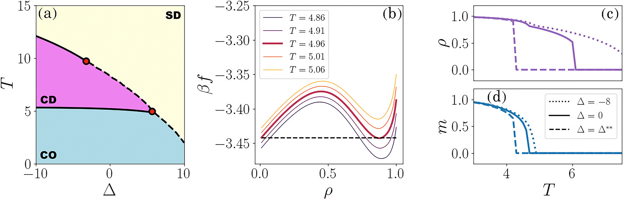 | ||
| Fig. 5 Mean-field results at K/J = 3.0 (a) equilibrium phase diagram in the (Δ,T) plane. The two red circles highlight the location of the two multicritical points, (Δ*,T*) = (−4.10,10.13) and (Δ**,T**) = (6.00,4.83) (b) density dependence of the free energy at Δ = Δ**. The two equal-height minima displayed by the red thickest curve signal the coexistence of a swollen ρ = 0 and a compact ρ = 0.87 phase. (c) and (d) Temperature dependence of the polymer's density ρ (c) and magnetization m (d) for Δ = −8 (i.e. crossing the two continuous phase boundaries), Δ = 0 (crossing the continuous CO/CD boundary and the first-order CD/SD boundary) and Δ = Δ* (crossing the multicritical point). | ||
This concludes our mean-field analysis. In the next section, we ask whether the rich scenario obtained within the mean-field theory is confirmed by the numerical results of a 3D lattice model magnetic polymer simulated using Monte Carlo methods.
IV. Numerical results
To simulate the model defined by eqn (2) in 3D space, we consider the set of self-avoiding walks on a cubic lattice where each node is decorated by a spin variable Si, which can take on the values 0, ±1. The set of configurations {γ,{S}} is sampled by a Monte Carlo (MC) algorithm based on a collection of elementary moves. These are: (i) pivot moves, essential for the ergodicity of the algorithm;16 (ii) a set of local Verdier–Stockmayer-style moves17 that are known to increase the mobility of the Markov chain in proximity of compact phase;18 (iii) a spin flip or Glauber dynamics to update the spin configurations along the walk. For an N-steps walk, an MC step (sometimes called sweep) consists of attempting 1 pivot moves intercalated by N/4 local moves and N spin updates. By using a Metropolis heat bath sampling with β ≡ kBT, the resulting Markov chain at temperature T is expected to converge to the equilibrium distribution | (10) |
 are given by eqn (1) and (2) respectively.
To enhance the sampling efficiency, we implement a multiple Markov chain algorithm. This approach, also known as replica exchange or parallel tempering algorithm, involves running Np parallel Markov chains, each at a distinct, fixed temperature T. A coupling between the Markov chains is established by trying to swap the configurations between chains that are contiguous in temperature space. By using a suitable swap protocol (here we have attempted a swap each 5 × 10³ MC steps, a number sufficiently high to avoid significant correlations between pairs of replicas) one can show that the collection of parallel Markov chains is itself a Markov chain whose stationary distribution is the product of the Boltzmann distribution along each chain (see ref. 18–21).
For each value of the parameter K considered (at fixed J = 1), we sample every M = 50 MC steps and along Np ≈ 30 parallel chains for systems of size N ∈ {50, 100, 200, 300, 400}. This amounts to a total of at least 2 × 10⁷ sampled configurations for each value of the set of parameters (N,K,J).
For each multiple Markov chain run we measure observables describing the state of the system. To characterise the polymer conformation, we compute the average number of contacts 〈c〉 – i.e., the number of pairs of nearest-neighbor lattice nodes occupied by the polymer that are not contiguous along the polymer backbone –, its variance per monomer Var(c) ≡ (〈nc2〉 − 〈nc〉2)/N, and the mean squared radius of gyration
 | (11) |
 is the position of the centre of mass and Ri is the position of the i-th monomer. To monitor the magnetic properties of the system, we estimate the degree of dilution, i.e., the concentration of neutral spins x = 1 − 〈S2〉, the magnetization per spin
  , and the magnetic susceptibility per spin
  . Finally, we also computed the average total energy 〈E〉 and the specific heat
  .
.
To locate the phase boundaries, we look at the T dependence of the specific heat, the magnetic susceptibility, and the variance of the number of contacts. We further perform a finite-size scaling (FSS) analysis on the specific heat, the magnetic susceptibility, the variance of the contacts, and the radius of gyration. FSS theory predicts, for instance, that the location of the peaks of the specific heat, T*(N), shifts towards the critical temperature Tc as N → ∞, as
 | (12) |
For a continuous phase transition, such as, for instance, the polymer Θ-point transition,22 we know that α = 0. Hence, by plotting  , a linear convergence toward the critical temperature is expected. On the contrary, a first-order transition corresponds to the value α = 1, which implies that T*(N) vs. 1/N should display a linear behaviour.
Similarly, we plot the value of the peaks of C, χM, and Var(c)/N. FSS predicts that these peaks behave in the proximity of the critical region (i.e., for N large enough) as
 | (13) |
![[thin space (1/6-em)]](https://www.rsc.org/images/entities/char_2009.gif) N, a linear growth is expected.
N, a linear growth is expected.
In addition, we estimate the order of the transitions by computing the fourth-order Binder cumulant of the distribution function of a given observable O: Bn(O) = 1 − 〈O4〉/3〈O2〉2. According to FSS theory, the location of the minimum of Bn(O) may be extrapolated to estimate the transition point. Importantly, if the phase transition is continuous, the values of Bn(O) at the minimum should asymptotically approach 2/3 with increasing N. In contrast, it should go to another limit if the transition is first-order.23
We estimate the errors associated with each observable O by using the corresponding integrated autocorrelation times τO. Some estimates of τO (given in units of the sampling, i.e., each M = 50 attempted pivot moves for O = E,m,RG) are reported in Appendix B for Δ = −5, 0 and 6, respectively (see Tables 1–3): as expected, sampled configurations are increasingly more correlated as T is decreased. At the lowest values of T, the simulations performed yield only a few hundred fully uncorrelated configurations. This impacts on the size of the error bars that increase rapidly as T decreases, as exemplified in Fig. 13 of the Appendix. To show the trends of the various observables more clearly, the error bars have been omitted from the other figures.
Although simulating polymers on the lattice is more efficient computationally compared to off-lattice models, a full numerical exploration of the (Δ,T) plane, even for a single specific K/J value, is still virtually impossible. We therefore restrict ourselves to the case K/J = 3, where the mean-field approximation suggests the emergence of a rich phase diagram with multiple phase transitions and critical points.
In particular, we focus on the CO/CD and CD/SD phase transitions at different values of Δ (Δ = −5, 0, 6).
A. Simulations for K/J = 3, Δ = −5
For negative values of Δ, neutral spins are not favourable and the dilution is weak; here, mean-field theory predicts the presence of two continuous phase transitions (see Fig. 5a). In Fig. 6 we report snapshots of typical configurations at T = 2.2, T = 4.5, and T = 10, where we expect the system to be, at equilibrium, in the CO, CD, and SD phases, respectively. The snapshots confirm the presence of all three phases, and importantly of the CD phase for the intermediate T = 4.5 temperature. More quantitatively, we looked at the T dependence of the specific heat (see Fig. 7a): the presence of two consecutive phase transitions is suggested by two sets of peaks whose heights increase with N. The fact that the set of peaks at low values of T refers to the CO/CD transition is confirmed by the concomitant formation of peaks in the magnetic susceptibility (see Fig. 12a in the Appendix). Instead, the set of peaks at high values of T corresponds to the CD/SD phase transition, since the variance of the number of contacts shows similar behavior in the same range of temperatures (see Fig. 12b in the Appendix). | ||
Fig. 6 Snapshots of typical MC configurations of a magnetic self-avoiding walk with N = 400, K/J = 3 and Δ = −5. The three panels were sampled respectively in the CO (left, T = 2.2), CD (middle, T = 4.5), and SD (right, T = 10) equilibrium phases. Red, white, and blue monomers correspond to spin values S = −1, 0 and 1, respectively. Note that in the CO phase, the polymer is greatly packed and almost all the monomers carry the same spin value; because of the ![[Doublestruck Z]](https://www.rsc.org/images/entities/char_e17d.gif) 2 symmetry, the two values of the magnetization m = ±1 can occur with equal probability. 2 symmetry, the two values of the magnetization m = ±1 can occur with equal probability. | ||
 | ||
Fig. 7 Monte Carlo results for K/J = 3, Δ = −5. In panels (a)–(c), different curves refer to different values of N (see legend in (b)). (a) Variance of the total energy C/β as a function of T. The estimated locations of the maxima are highlighted by larger coloured circles. (b) RG2/N2/3 as a function of T. Crossings with the N = 400 curve are highlighted by blue squares. (c) Binder cumulant of the energy Bn(E) as a function of T. Minima are marked with green (CO/CD transition) and violet (CD/SD transition) squares. (d) Values of T at which Bn(E) has a minimum as a function of N−1/2. (e) Values of T at which different quantities (reported in the legend) display a maximum as a function of  ; they converge linearly to an asymptotic (N → ∞) value. We extrapolate estimates for the transition temperatures and highlight the mean-field predictions T1 and T2 on the y-axis. (f) Height of the maxima of different quantities (reported in the legend; note that, for C/β, we plot ; they converge linearly to an asymptotic (N → ∞) value. We extrapolate estimates for the transition temperatures and highlight the mean-field predictions T1 and T2 on the y-axis. (f) Height of the maxima of different quantities (reported in the legend; note that, for C/β, we plot  ) as a function of logN. ) as a function of logN. | ||
An observable that better describes the conformational properties of the polymer, but is not easily accessible through the mean-field calculations, is the statistical size of the chain, which we measured in terms of its mean-squared radius of gyration 〈RG2〉. Since in the two compact phases 〈RG2〉 ∼ N2/d, in Fig. 7b we report 〈RG2〉/N2/3 as a function of T. It can be seen that, at large values of T, the scaled curves increase with N. This is expected since 〈RG2〉 ∼ N2νSAW for polymers in the swollen phase, with νSAW ≈ 0.5889 > 1/2.24 On the other hand, at low values of T, where the polymer is in a compact (either disordered or ordered) phase, data for large polymers collapse onto a master curve. The finite N crossover between the SD and the CD phase is revealed by the crossings of these curves, whose location can be used as a further estimate of the location of the SD/CD phase transition.
In addition, we determine the nature of the transitions by looking at the Binder cumulant of the energy Bn(E) as a function of T (see Fig. 7c).23 The onset of two sets of minima further confirms the presence of two phase transitions. Moreover, as N increases, both sets seem to converge to the limiting value 2/3, a clear indication that both transitions are continuous (see Fig. 7d).
Finally, we provide estimates for the location of the phase boundaries via finite-size scaling (FSS). The plots reported in Fig. 7e and f corroborate the continuous nature of the transition, not only for the location of the maxima of C, χM and Var(c), but also for the value of the peaks for the same quantities, as well as the crossings of the RG curves. By averaging the set of extrapolated values over the different observables, we obtained Tc(SD/CD) = 8.2 ± 0.1 and Tc(CD/CO) = 4.08 ± 0.08. Note that both estimates are significantly smaller than the mean-field ones.
In summary, the MC findings for K/J = 3 and Δ = −5 corroborate the mean-field picture, namely the presence of three equilibrium phases with the SD/CD and CD/CO phase boundaries, both of which are continuous. Note that the presence of the CD phase in the 3D system occurs at values of K/J that are larger than those for which this phase is expected in MF (see Appendix C).
B. Simulations for K/J = 3, Δ = 0
Increasing Δ favors neutral spins, or in other words, dilution increases. At Δ = 0 the mean field theory predicts that there should once again be two phase transitions, an SD/CD and a CD/CO transition. Whilst the CD/CO transition remains continuous, the SD/CD transition is predicted to be discontinuous in this case (see Fig. 5).The corresponding MC results indeed show two sets of peaks in the specific heat, corresponding to two transitions. The height of both sets of peaks increases with N (see Fig. 8a). As for Δ = −5, the set of peaks at low values of T colocalises with the one observed in χM (see Fig. 12c) and hence refers to the CO/CD phase transition. The second set, occurring at higher values of T, originates from the corresponding non-monotonic behaviour of Var(c) (see Fig. 12d) and signals the SD/CD phase transition. This is confirmed by the crossings of the RG2/N2/3 curves (see Fig. 8b). Notably, both sets of minima observed in the Binder parameter of the energy (see Fig. 8c) converge (as N → ∞) to 2/3, as expected for a continuous phase transition (see Fig. 8d).
 | ||
Fig. 8 Monte Carlo results for K/J = 3, Δ = 0. In panels (a)–(c), different curves and points are as in Fig. 7. (a) Variance of the total energy C/β as a function of T. (b) RG2/N2/3 as a function of T. (c) Binder cumulant of the energy Bn(E) as a function of T. (d) Values of T at which Bn(E) has a minimum as a function of  . (e) Values of T at which different quantities (reported in the legend) display a maximum as a function of . (e) Values of T at which different quantities (reported in the legend) display a maximum as a function of  . We extrapolate estimates for the transition temperatures and highlight the mean-field estimates T1 and T2 on the y-axis. (f) Height of the maxima of different quantities (reported in the legend; for C/β, we plot . We extrapolate estimates for the transition temperatures and highlight the mean-field estimates T1 and T2 on the y-axis. (f) Height of the maxima of different quantities (reported in the legend; for C/β, we plot  ) as a function of logN. ) as a function of logN. | ||
Finally, the linear trends of the location of the peaks of C, χM, Var(c), and the crossings of the scaled Rg curves, once plotted as a function of  as well as the
  growth of the peaks’ heights (see Fig. 8e and f) corroborates this finding.
By averaging the extrapolated values of T*(N) on the different observables (see Fig. 8), we estimate Tc(SD/CD) = 7.3 ± 0.1 and Tc(CD/CO) = 4.106 ± 0.006. Note that, again, the estimated values are lower than the mean-field ones.
Therefore, the Monte Carlo results at Δ = 0 confirm the mean-field prediction for the CO/CD phase boundary. However, there is a discrepancy regarding the nature of the SD/CD phase transition: while the mean field theory predicts a first-order transition, the magnetic polymer model in 3D is suggestive of a second-order transition.
To understand more in-depth the relation between the mean field prediction and the behaviour of the system in 3D, we extended the MC investigation to Δ = 6.
C. Simulations for K/J = 3, Δ = 6
The mean-field theory predicts that, at Δ ≈ 6.00 and T ≈ 4.83, the system is at the multicritical point where the two first-order phase boundaries SD/CD and SD/CO meet the continuous phase transition line between CD and CO. According to what was observed at Δ = 0, we expect the 3D system to be in the region where the SD/CD and CD/CO boundaries are still well separated. We aim to verify whether the SD/CD boundary has become first-order as predicted by MF (see Fig. 5a).The onset of two distinct, although close, sets of peaks in the variance of the energy (see Fig. 9a) confirms the presence of two phase boundaries that, according to the concomitant developments of the peaks in χM/β and Var(c)/N, we can identify as the SD/CD and the CD/CO phase transitions, respectively (see Fig. 12e and f). The presence of the SD/CD transition at large values of T is corroborated by the crossings of the radius of gyration curves when scaled by N2/3, and by the minima of Bn(E) (see Fig. 9b and c).
 | ||
Fig. 9 Monte Carlo results for K/J = 3, Δ = 6. In panels (a)–(c), different curves and points are as in Fig. 7. (a) Variance of the total energy as a function of T. (b) RG2/N2/3 as a function of T. (c) Binder cumulant of the energy Bn(E) as a function of T. (d) Values of T at which Bn(E) has a minimum as a function of 1/N. (e) Values of T at which different quantities (reported in the legend) display a maximum as a function of 1/N. We extrapolate an estimate for the temperature corresponding to the CD/CO transition, highlighting the mean-field prediction Tc on the y-axis. (f) Height of the maxima of different quantities (reported in the legend; for C/β, we plot  ) as a function of N. ) as a function of N. | ||
We highlight that the set of minima of Bn(E) at high values of T, which were already rather shallow at Δ = 0, are not observed in this case since all curves rapidly approach the value 2/3 in that range of T. This suggests that the CD/CO phase boundary remains continuous.
Instead, at low values of T, the set of minima converges as N increases to a value that is far from 2/3 (see Fig. 9c and d): this is a clear signal that the CO/CD phase transition has now become first order. We remark that the mean-field calculations predicted a qualitatively different scenario, with a continuous CO/CD transition and a first-order CD/SD transition. The discontinuous nature of the CO/CD transition is confirmed by the trends of the location of the peaks of C/β, and χM, once plotted as a function of 1/N, as well as the linear dependence in N of the height of the peaks (see Fig. 9e and f). Thus, at Δ = 6 the 3D system shows a change of the nature of a phase boundary from continuous to first-order; however, we observe it for the CO/CD boundary, rather than for the CD/SD one. This suggests that thermal fluctuations have a strong effect on the phase behaviour of the system and qualitatively modify the mean-field picture at high values of the dilution parameter Δ, altering not only the location of the phase boundaries in the (Δ,T) plane but also their nature.
V. Conclusions
In this work, we have studied the equilibrium properties of a magnetic polymer endowed with a spin model (the Blume–Emery–Griffiths). There are three terms in the Hamiltonian, which respectively describe: (i) exchange interactions between ±1 spins, favouring alignment (i.e., ferromagnetic interactions), (ii) self-attraction between monomers and (iii) relative balance between neutral and ±1 spins, which we refer to as dilution (as increasing dilution increases the average portion of neutral spins on the chain).We first studied this problem using a mean-field (MF) approximation. The resulting MF phase diagram is very rich, and features phase boundaries whose nature and location depend on the degree of dilution Δ and the relative strength of the self-attraction parameter over the ferromagnetic one K/J. In addition to the previously reported swollen-disordered (SD) and compact-ordered (CO) phases,4,6,7 the MF results reveal the presence of an equilibrium phase characterized by a globular polymer conformation with zero magnetization. This compact-disordered (CD) phase was not observed at equilibrium in previously studied models of magnetic polymers where the conformational transitions were triggered exclusively by the ferromagnetic coupling J.
To validate these findings and to test the validity of the MF phase diagram against thermal fluctuations, we performed Monte Carlo simulations of the corresponding model on the cubic lattice. We considered a fixed value of the K/J ratio (K/J = 3), at which the MF analysis displays a rich phase diagram as a function of the dilution parameter Δ (see Fig. 5). Our results show that upon increasing Δ, the MC picture fundamentally deviates from the mean-field one. At Δ = −5, where dilution is weak, we confirm the presence and continuous nature of both phase transitions (CO/CD and CD/SD) predicted by the mean-field (MF) theory. At Δ = 0, the nature of the CO/CD transition is confirmed, and the transition temperature appears to be independent of Δ (as in mean-field). However, the CD/SD transition retains its continuous nature, at variance with the mean-field prediction (see Fig. 5). Upon increasing the dilution further (Δ = 6), we find that the scenario predicted by the MC simulations deviates even more from the mean-field, as the CO/CD transition becomes first-order, whereas the CD/SD remains second order – this is the opposite of what MF predicts. Results and comparison are summarized in Fig. 10.
 | ||
| Fig. 10 Estimated phase diagram of the magnetic polymer model on the cubic lattice (K/J = 3) from Monte Carlo simulations. The solid and dashed lines represent, respectively, the continuous and discontinuous phase boundaries, as estimated by the Monte Carlo simulations, and the stable SD, CD, and CO phases are enclosed between these lines. These regions should be compared with the uniformly colored zones, which correspond to the values of (T,Δ) at which the same phases are predicted to be stable by the mean-field (MF) theory. The red circle is the expected location of the multicritical point (Δ*,T*). | ||
Our results show that fluctuations are important in 3D, as they modify the nature of the transitions as predicted by the MF theory, most notably for the CO/CD transition. The traditional BEG model on the lattice (i.e., not on a polymer) also yields qualitative differences between mean-field calculations and Monte Carlo simulations have also been found on the lattice: for example, it has been shown that tricritical points may disappear, upon varying K/J, when moving from the microcanonical to the canonical ensemble.25 As such, the discrepancies between MC and MF reported here may align with what has been found for the traditional BEG model. An additional important element that is not present in the original BEG problem is the entropy of the polymer configurations that is encoded in the term  (see Appendix A after eqn (18)). In our MF approach, this term is approximated by restricting the sum to the subset of the Hamiltonian walks (see Appendix A). The Hamiltonian walk approximation is quite appropriate in the case of polymers in compact phases, but underestimates the configurational entropy of the polymer in extended phases. We believe that a possible improvement of the MF approximation should require a more precise estimate of this entropic term.
It is also of interest to discuss the results found here in the context of biophysics, where magnetic polymer models have previously been used to study the spreading of epigenetic marks on chromatin,9,10,13,26,27 the DNA–protein complex which provides the building block of eukaryotic chromosomes. With respect to those models, the main additional ingredient considered here is the ±1 spin dilution, or the presence of neutral spins, corresponding to inert or unmarked chromatin beads, devoid of active and inactive epigenetic marks (which can in turn be modeled as ±1 spins). This feature can effectively mimic the fact that marks need to be deposited by enzymes, which are limited in number in a living cell. Our results show that dilution leads to the emergence of the compact disordered phase, which was previously only found with polymer models out of thermodynamic equilibrium. The CD phase can represent chromatin regions compactified by bridging proteins which are not epigenetic readers or writers (an example of such a bridge could be cohesin or another SMC protein). Another important finding is that changing dilution can lead to a switch between a continuous and a discontinuous transition between the compact ordered and the compact disordered phase. The order of the transition is relevant to the physics of chromatin, as a first-order transition endows the system with memory,10 such that, for instance, it is now possible, within our model, for a compact and disordered state to retain its state following replication.
In the future it would be interesting to investigate numerically the 2D case, where fluctuations can further affect the mean-field predictions, to see if the phase diagram changes also qualitatively. From the biophysics viewpoint, an avenue to extend our study would also be to introduce epigenetic bookmarks as in ref. 13, and investigate whether this can lead to the formation of stable unmarked inert, alongside marked active or inactive, epigenetic domains in chromatin.
Data availability
The data supporting this article have been included as part of the Appendices.Conflicts of interest
There are no conflicts to declare.Appendices
A: Mean-field theory
 | (14) |
| Dϕ ≡ (2π)−N/2(βJ)−N/2det(Λ)−1/2dNϕ | (15) |
| Dα ≡ (2π)−N/2(βK)−N/2det(Λ)−1/2dNα. | (16) |
By summing over all possible spin configurations {Si} we get
 | (17) |
 | (18) |
 depends on a given SAW it cannot be computed exactly. We can, however, approximate it by restricting the sum to the subset of space-filling SAWs within a volume V known as Hamiltonian walks.4,28 For a given Hamiltonian walk, Λγ simplifies to the adjacency matrix of the underlying lattice with coordination number z. This approximation is appropriate for SAWs in the compact phase, which is space-filling. However, it is rather strong for swollen SAWs: we mitigate this issue by replacing the lattice coordination number z with ρz, thus considering SAWs that, having ρ = N/V < 1, display an effective lower mean number of nearest neighbors. This gives
 | (19) |
 | (20) |
By plugging eqn (19) and (20) in eqn (18) we obtain the mean-field partition function as
 | (21) |
By taking the −1/βlog of eqn (21) and dividing by the system's size N we obtain the mean-field free energy density of eqn (3).
 | (22) |
 | (23) |
 | (24) |
Finally, by inserting eqn (24) in eqn (3), Taylor expanding around ρ = 0 and computing the osmotic pressure as
 | (25) |
| βΠ(β,ρ) = B1(β,ρ)ρ + B2(β,ρ)ρ2 + B3(β,ρ)ρ3 + ⋯ | (26) |
| B2(β,Δ) = 1, | (27a) |
 | (27b) |
 | (27c) |
 | (28a) |
 | (28b) |
 | (28c) |
 | (29) |
Inserting eqn (22) and (29) in eqn (3) and expanding the result around ϕ = 0 we find the polynomial expression
| f(β,Δ) = f0 + a(β,Δ)ϕ2 + b(β,Δ)ϕ4 + O(ϕ6). | (30) |
In Fig. 11 we show the contour plots of the coefficient b(β,Δ) and c(β,Δ) for the four different values of the ratio K/J discussed in the main text. Condition a(Δ,T) = 0 is represented on the plane as black lines. For all K/J considered, this locus of points is made of straight and curved lines, originating from Δ = 0 and T = 0. Condition b(Δ,T) = 0 is displayed instead as a white line. Both this white line and the curved black line display a horizontal asymptote as Δ → −∞. From Landau's theory of phase transitions, critical points arise when a(Δ,T) = 0, b(Δ,T) > 0, and c(Δ,T) > 0. Instead, a tricritical point is observed when a(Δ,T) = b(Δ,T) = 0 and c(Δ,T) > 0. Thus, despite the presence of the straight black line, no critical points are observed in the green regions where c(Δ,T) < 0 (see Fig. 11b, d, f and g). When K/J = 0.8 (Fig. 11a and b), the black line lies totally inside the blue region, where b(Δ,T) < 0: no critical points appear on the CO/CD phase boundary. When K/J = 1.8 (Fig. 11c and d), the black line intercepts the white one when Δ → −∞: thus, a tricritical point is observed when there are no neutral states. Indeed, we compute, numerically, the values of K/J and β such that a continuous CO/CD transition occurs: we solve the system of equations
 | (31) |
 | (32) |
 | (33) |
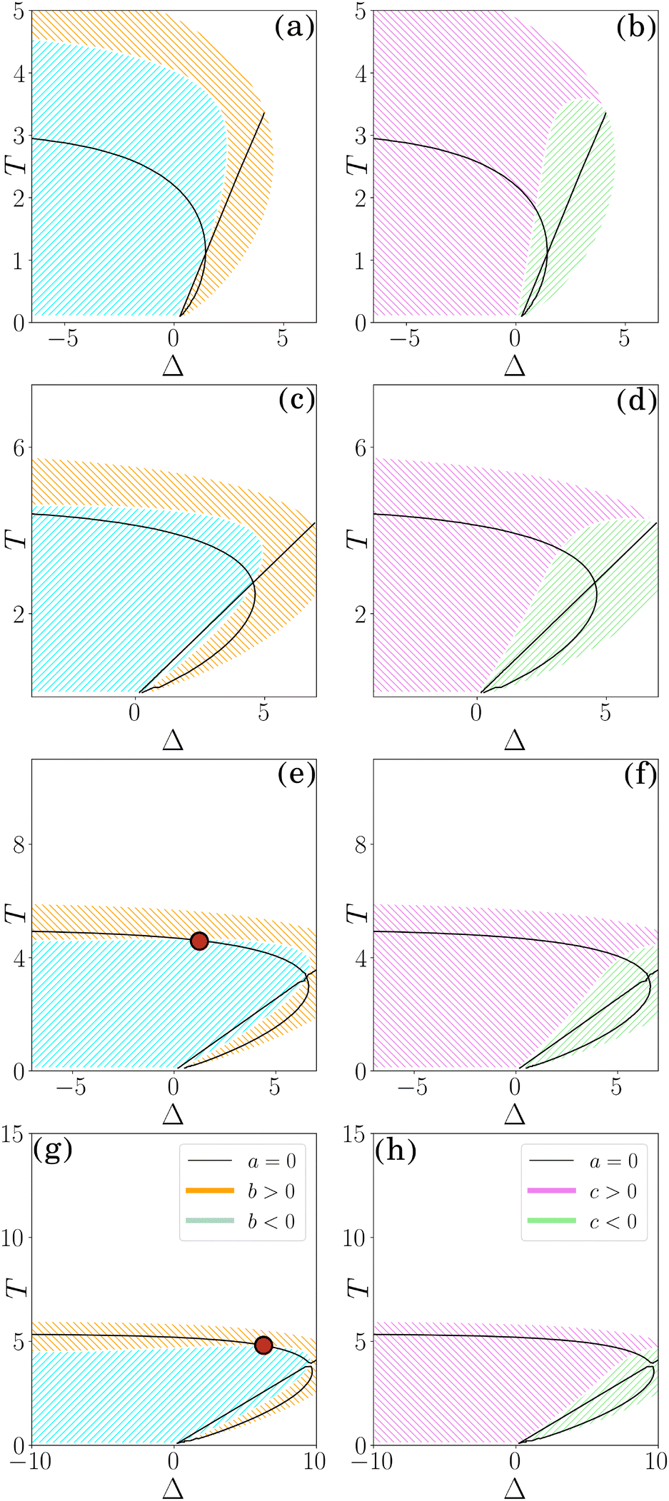 | ||
| Fig. 11 Contour plots of the coefficients b(Δ,T) and c(Δ,T) for K/J = 0.8 (a) and (b), 1.8 (c) and (d), 2.3 (e) and (f) and 3.0 (g) and (h). In all panels, red dots mark the position of multicritical points, while black lines mark the values where a(Δ,T) = 0. In the full white regions the functions b(Δ,T) and c(Δ,T) are not defined. Colored-white patterned regions (see legend in panels (g) and (h)) represent the regions where b(Δ,T) and c(Δ,T) have definite sign, separated by white lines marking either b(Δ,T) = 0 (left column) or c(Δ,T) = 0 (right column). | ||
By increasing the K/J ratio, the tricritical point moves towards higher values of Δ, and in Fig. 11e it is represented as a red dot. Increasing further the K/J ratio, the tricritical point moves further towards the right (Fig. 11g), but in the phase diagram shown in Fig. 5a a CO/CD tricritical point is not observed because of the presence of a first-order CO/SD phase transition.
B: Monte Carlo simulations
 | ||
| Fig. 12 (a), (c) and (e) Magnetic susceptibility per spin χM/β and (b), (d) and (f) variance of the number of contacts Var(c)/N as a function of T for the systems studied in the main text, K/J = 3 and (a) and (b) Δ = −5, (c) and (d) Δ = 0, (e) and (f) Δ = 6. | ||
Instead, the sets of peaks of Var(c)/N always happen at high values of T and correspond to the CD/SD transition. In this case, the positions of these maxima shift to lower values of T with increasing Δ, which is also in qualitative agreement with the mean-field predictions.
| T | τ E | τ M | τ RG |
|---|---|---|---|
| 2.00 | 5.0(4) × 104 | 2.0(2) × 105 | 8.0(8) × 104 |
| 2.13 | 2.0(2) × 104 | 1.2(5) × 104 | 6.0(3) × 103 |
| 2.27 | 3.0(1) × 103 | 5.0(2) × 103 | 2.7(9) × 103 |
| 2.38 | 2.0(8) × 103 | 2.7(8) × 103 | 2.2(7) × 103 |
| 2.50 | 1.1(4) × 103 | 4.5(7) × 102 | 1.3(2) × 103 |
| 2.63 | 4.4(10) × 102 | 2.3(2) × 102 | 1.1(2) × 103 |
| 2.78 | 2.3(4) × 102 | 2.3(2) × 102 | 9.0(2) × 102 |
| 2.94 | 1.0(1) × 102 | 1.0(8) × 102 | 7.0(1) × 102 |
| 3.13 | 6.7(6) × 101 | 3.9(2) × 101 | 6.0(1) × 102 |
| 3.33 | 4.7(4) × 101 | 1.03(3) × 101 | 6.0(1) × 102 |
| 3.45 | 3.9(4) × 101 | 4.92(8) × 100 | 5.8(8) × 102 |
| 3.57 | 3.2(3) × 101 | 2.39(3) × 100 | 5.6(7) × 102 |
| 3.70 | 2.8(2) × 101 | 1.202(8) × 100 | 5.0(6) × 102 |
| 3.85 | 2.9(2) × 101 | 7.62(3) × 10−1 | 4.7(6) × 102 |
| 4.00 | 2.9(2) × 101 | 5.9(2) × 10−1 | 4.3(6) × 102 |
| 4.17 | 3.1(2) × 101 | 5.29(1) × 10−1 | 3.9(5) × 102 |
| 4.35 | 3.1(2) × 101 | 5.1(1) × 10−1 | 3.7(5) × 102 |
| 4.55 | 3.2(2) × 101 | 5.02(8) × 10−1 | 3.9(5) × 102 |
| 4.76 | 3.4(2) × 101 | 5.01(8) × 10−1 | 3.9(5) × 102 |
| 5.00 | 1.7(8) × 101 | 5.01(7) × 10−1 | 6.8(4) × 101 |
| 5.13 | 1.6(8) × 101 | 5.01(1) × 10−1 | 6.3(4) × 101 |
| 5.26 | 1.72(9) × 101 | 5.01(7) × 10−1 | 6.9(6) × 101 |
| 5.41 | 1.9(1) × 101 | 5.0(4) × 10−1 | 7.0(5) × 101 |
| 5.56 | 2.1(1) × 101 | 5.0(4) × 10−1 | 7.2(6) × 101 |
| 5.71 | 2.4(2) × 101 | 5.0(1) × 10−1 | 7.5(6) × 101 |
| 5.88 | 3.0(2) × 101 | 5.0(4) × 10−1 | 7.7(7) × 101 |
| 6.06 | 3.5(3) × 101 | 5.0(4) × 10−1 | 8.0(7) × 101 |
| 6.25 | 4.0(3) × 101 | 5.01(1) × 10−1 | 7.7(7) × 101 |
| 6.45 | 4.7(4) × 101 | 5.01(1) × 10−1 | 6.7(5) × 101 |
| 6.67 | 5.6(4) × 101 | 5.02(1) × 10−1 | 6.7(5) × 101 |
| 6.90 | 7.0(5) × 101 | 5.02(1) × 10−1 | 6.8(5) × 101 |
| 7.14 | 6.6(5) × 101 | 5.0(4) × 10−1 | 5.7(4) × 101 |
| 7.41 | 4.3(2) × 101 | 5.01(7) × 10−1 | 3.3(2) × 101 |
| 7.69 | 2.7(1) × 101 | 5.0(4) × 10−1 | 1.9(7) × 101 |
| 8.00 | 1.52(5) × 101 | 5.0(4) × 10−1 | 1.0(3) × 101 |
| 8.33 | 7.8(2) × 100 | 5.0(4) × 10−1 | 4.9(1) × 100 |
| T | τ E | τ M | τ RG |
|---|---|---|---|
| 2.22 | 1.6(5) × 103 | 2.0(2) × 104 | 6.0(4) × 103 |
| 2.33 | 6.0(2) × 102 | 7.0(4) × 103 | 2.0(1) × 103 |
| 2.50 | 2.2(4) × 102 | 2.2(8) × 103 | 6.0(1) × 102 |
| 2.63 | 1.0(2) × 102 | 9.0(2) × 102 | 3.4(7) × 102 |
| 2.70 | 5.7(6) × 101 | 6.0(2) × 102 | 3.6(7) × 102 |
| 2.86 | 3.7(4) × 101 | 2.4(5) × 102 | 2.1(4) × 102 |
| 3.03 | 1.5(1) × 101 | 6.6(8) × 101 | 3.3(4) × 101 |
| 3.13 | 1.17(7) × 101 | 3.3(2) × 101 | 1.5(2) × 102 |
| 3.23 | 1.02(6) × 101 | 2.2(1) × 101 | 2.3(2) × 101 |
| 3.33 | 9.3(5) × 100 | 1.31(5) × 101 | 3.6(4) × 101 |
| 3.57 | 6.8(3) × 100 | 2.94(4) × 100 | 3.3(3) × 101 |
| 3.85 | 5.3(2) × 100 | 7.82(5) × 10−1 | 4.3(3) × 101 |
| 4.00 | 4.4(2) × 100 | 5.77(2) × 10−1 | 3.5(2) × 101 |
| 4.17 | 4.2(2) × 100 | 5.28(3) × 10−1 | 3.3(2) × 101 |
| 4.35 | 4.4(2) × 100 | 5.06(2) × 10−1 | 2.3(2) × 101 |
| 4.55 | 4.5(2) × 100 | 5.01(1) × 10−1 | 2.2(2) × 101 |
| 4.76 | 5.4(2) × 100 | 5.0(6) × 10−1 | 1.7(1) × 101 |
| 5.00 | 6.5(3) × 100 | 5.0(6) × 10−1 | 1.8(1) × 101 |
| 5.26 | 8.7(4) × 100 | 5.0(6) × 10−1 | 2.4(1) × 101 |
| 5.56 | 1.52(1) × 101 | 5.0(6) × 10−1 | 3.4(3) × 101 |
| 5.88 | 2.4(2) × 101 | 5.0(6) × 10−1 | 3.7(2) × 101 |
| 6.25 | 3.6(2) × 101 | 5.0(6) × 10−1 | 3.8(2) × 101 |
| 6.67 | 2.9(1) × 101 | 5.01(1) × 10−1 | 2.4(1) × 101 |
| 7.14 | 9.5(3) × 100 | 5.03(2) × 10−1 | 7.0(2) × 100 |
| 7.41 | 5.3(2) × 100 | 5.0(6) × 10−1 | 3.7(1) × 100 |
| 7.69 | 3.3(1) × 100 | 5.0(6) × 10−1 | 2.1(4) × 100 |
| 8.00 | 2.09(5) × 100 | 5.0(6) × 10−1 | 1.51(3) × 100 |
| 8.33 | 1.78(4) × 100 | 5.0(6) × 10−1 | 1.33(2) × 100 |
| T | τ E | τ M | τ RG |
|---|---|---|---|
| 2.33 | 1.3(2) × 102 | 2.5(8) × 103 | 4.9(1) × 102 |
| 2.50 | 2.9(3) × 101 | 7.0(2) × 102 | 1.2(1) × 102 |
| 2.703 | 7.3(4) × 100 | 1.1(2) × 102 | 3.9(4) × 101 |
| 2.8 | 4.4(2) × 100 | 4.1(3) × 101 | 2.0(1) × 101 |
| 3.03 | 2.67(9) × 100 | 2.1(1) × 101 | 1.41(7) × 101 |
| 3.23 | 2.07(6) × 100 | 9.8(4) × 100 | 9.8(4) × 100 |
| 3.33 | 2.02(5) × 100 | 6.0(2) × 100 | 8.4(3) × 100 |
| 3.57 | 1.83(4) × 100 | 1.13(2) × 100 | 7.2(3) × 100 |
| 3.70 | 2.03(6) × 100 | 6.8(4) × 10−1 | 6.4(2) × 100 |
| 3.85 | 2.35(8) × 100 | 5.5(3) × 10−1 | 6.1(2) × 100 |
| 4.00 | 2.8(1) × 100 | 5.1(1) × 10−1 | 5.9(2) × 100 |
| 4.17 | 3.08(9) × 100 | 5.06(2) × 10−1 | 6.1(2) × 100 |
| 4.35 | 4.7(2) × 100 | 5.0(8) × 10−1 | 6.2(2) × 100 |
| 4.44 | 5.7(2) × 100 | 5.0(8) × 10−1 | 6.8(2) × 100 |
| 4.55 | 8.4(4) × 100 | 5.0(8) × 10−1 | 8.0(3) × 100 |
| 4.65 | 1.1(6) × 101 | 5.0(8) × 10−1 | 9.8(4) × 100 |
| 4.76 | 1.3(6) × 101 | 5.0(8) × 10−1 | 1.1(5) × 101 |
| 4.88 | 1.25(6) × 101 | 5.0(8) × 10−1 | 8.8(4) × 100 |
| 5.00 | 7.8(3) × 100 | 5.04(2) × 10−1 | 5.4(2) × 100 |
| 5.05 | 6.8(3) × 100 | 5.0(2) × 10−1 | 4.4(1) × 100 |
| 5.13 | 4.9(2) × 100 | 5.0(8) × 10−1 | 3.3(1) × 100 |
| 5.26 | 3.17(1) × 100 | 5.0(8) × 10−1 | 2.1(6) × 100 |
| 5.41 | 2.68(9) × 100 | 5.0(8) × 10−1 | 1.55(3) × 100 |
| 5.56 | 2.14(7) × 100 | 5.01(1) × 10−1 | 1.22(2) × 100 |
| 5.88 | 1.74(6) × 100 | 5.0(1) × 10−1 | 9.9(1) × 10−1 |
| 6.250 | 1.38(4) × 100 | 5.0(8) × 10−1 | 8.68(8) × 10−1 |
| 6.67 | 1.06(2) × 100 | 5.0(8) × 10−1 | 8.1(7) × 10−1 |
| 8.33 | 9.2(2) × 10−1 | 5.0(8) × 10−1 | 7.2(7) × 10−1 |
These estimates contribute to the error bars of the observables since the variance of an observable O is 2τO larger than it would be for statistically independent samples. In Tables 1–3 we report the values of τO for the total energy, the magnetisation, and the radius of gyration.
The T dependence of some observables with their corresponding error bars is exemplified in Fig. 13, where we reported the data at Δ = 0. We note that the largest error bars appear at low temperatures: this is because of the difficulty in efficiently sampling the system there, due to the large autocorrelation. Error bars are also large at temperatures close to the critical point, where critical slowing down is expected.
 | ||
| Fig. 13 Estimations of (a) C/β, (b) χM/β and (c) RG2, complete with error bars, when K = 3, J = 1, Δ = 0 and N = 400. | ||
C: Monte Carlo simulations for the case K/J = 0.8 and Δ = −6
Here we present some preliminary results for MC simulations regarding the intermediate case K/J = 0.8 and Δ = −6. As reported in Fig. 2a, the mean field theory predicts the existence of a CD phase, which borders the CO phase with a discontinuous transition and the SD phase with a continuous transition.The presence of a unique peak in the specific heat (see Fig. 14a) suggests that, at variance with the MF prediction, the simulated 3D system does not display an intervening CD phase between the CO and SD phases. The presence of the single SD/CO transition is confirmed by the crossing of the radius of gyration curves once scaled by N2/3 (see Fig. 14b). Additionally, the fact that the minima of the Binder cumulant curves (reported in Fig. 14c) tend to 2/3 as N → ∞, as shown in Fig. 14d, suggests that the SD/CO transition is continuous (as in the case K/J = 3 and Δ = 6). The continuous character of the transition is further corroborated both by the shift of the locations of the maxima of CV, χM and Var(c) (see also the crossing points of the Rg2/N2/3 curves) as a function of  (see Fig. 14e) and by the growth of the heights of these observables as a function of logN (see (Fig. 14f)).
 | ||
Fig. 14 Monte Carlo results for K/J = 0.8, Δ = −6. In panels (a)–(c), different curves and points are as in Fig. 7. (a) Variance of the total energy as a function of T. (b) RG2/N2/3 as a function of T. (c) Binder cumulant of the energy Bn(E) as a function of T. (d) Values of T at which Bn(E) has a minimum as a function of  . (e) Values of T at which different observables (reported in the legend) display a maximum as a function of . (e) Values of T at which different observables (reported in the legend) display a maximum as a function of  . We extrapolate an estimate for the temperature corresponding to the CD/CO transition. (f) Height of the maxima of different quantities (reported in the legend; for C/β, we plot . We extrapolate an estimate for the temperature corresponding to the CD/CO transition. (f) Height of the maxima of different quantities (reported in the legend; for C/β, we plot  ) as a function of logN. ) as a function of logN. | ||
These findings, complemented with those reported in the text for K/J = 3, suggest that in the 3D system the CD phase will appear at a value of the ratio K/J between 0.8 and 3.0.
Acknowledgements
E. O. acknowledges support from grant PRIN 2022R8YXMR funded by the Italian Ministry of University and Research. The authors acknowledge CloudVeneto for the use of computing and storage facilities.References
- A. Rajca, J. Wongsriratanakul and S. Rajca, Magnetic ordering in an organic polymer, Science, 2001, 294(5546), 1503–1505 CrossRef CAS PubMed.
- J. S. Miller, Organic-and molecule-based magnets, Mater. Today, 2014, 17(5), 224–235 CrossRef CAS.
- B. W. Boudouris and Y. Joo, Spin-Active and Magnetic Polymers, ACS Macro Lett., 2024, 13(7), 832–833 CrossRef CAS.
- T. Garel, H. Orland and E. Orlandini, Phase diagram of magnetic polymers, Eur. Phys. J. B, 1999, 12(2), 261–268 CrossRef CAS.
- M. B. Luo, Finite-size scaling analysis on the phase transition of a ferromagnetic polymer chain model, J. Chem. Phys., 2006, 124(3), 034903 CrossRef PubMed.
- A. Papale and A. Rosa, The Ising model in swollen vs. compact polymers: Mean-field approach and computer simulations, Eur. Phys. J. E:Soft Matter Biol. Phys., 2018, 41, 1–9 CrossRef CAS.
- D. P. Foster and D. Majumdar, Critical behavior of magnetic polymers in two and three dimensions, Phys. Rev. E, 2021, 104(2), 024122 CrossRef CAS.
- S. Rudra, D. P. Foster and S. Kumar, Critical behavior of magnetic polymers on the three-dimensional Sierpiński Gasket, Phys. Rev. E, 2023, 108(4), L042502 CrossRef CAS PubMed.
- D. Colì, E. Orlandini, D. Michieletto and D. Marenduzzo, Magnetic polymer models for epigenetics-driven chromosome folding, Phys. Rev. E, 2019, 100(5), 052410 CrossRef.
- D. Michieletto, E. Orlandini and D. Marenduzzo, Polymer model with epigenetic recoloring reveals a pathway for the de novo establishment and 3D organization of chromatin domains, Phys. Rev. X, 2016, 6(4), 041047 Search PubMed.
- I. Lifshitz, A. Y. Grosberg and A. Khokhlov, Some problems of the statistical physics of polymer chains with volume interaction, Rev. Mod. Phys., 1978, 50(3), 683 CrossRef CAS.
- G. J. Filion, J. G. van Bemmel, U. Braunschweig, W. Talhout, J. Kind and L. D. Ward, et al., Systematic protein location mapping reveals five principal chromatin types in Drosophila cells, Cell, 2010, 143(2), 212–224 CrossRef CAS.
- D. Michieletto, D. Colì, D. Marenduzzo and E. Orlandini, Nonequilibrium theory of epigenomic microphase separation in the cell nucleus, Phys. Rev. Lett., 2019, 123(22), 228101 CrossRef CAS PubMed.
- R. Nakanishi and K. Hukushima, Emergence of compact disordered phase in a polymer Potts model, Phys. Rev. E, 2024, 109(1), 014405 CrossRef CAS PubMed.
- M. Blume, V. J. Emery and R. B. Griffiths, Ising Model for the λ Transition and Phase Separation in He3–He4 Mixtures, Phys. Rev. A, 1971, 4(3), 1071–1077 CrossRef.
- N. Madras, A. Orlitsky and L. A. Shepp, Monte Carlo generation of self-avoiding walks with fixed endpoints and fixed length, J. Stat. Phys., 1990, 58(1), 159–183 CrossRef.
- P. H. Verdier and W. H. Stockmayer, Monte Carlo calculations on the dynamics of polymers in dilute solution, J. Chem. Phys., 1962, 36(1), 227–235 CrossRef CAS.
- M. C. Tesi, J. E. Janse van Rensburg, E. Orlandini and S. G. Whittington, Monte Carlo Study of the Interacting Self-Avoiding Walk Model in Three Dimensions, J. Stat. Phys., 1996, 82, 155–181 CrossRef.
- C. J. Geyer, Practical markov chain monte carlo, Stat. Sci., 1992, 473–483 Search PubMed.
- K. Hukushima and K. Nemoto, Exchange Monte Carlo method and application to spin glass simulations, J. Phys. Soc. Jpn., 1996, 65(6), 1604–1608 CrossRef CAS.
- U. H. Hansmann, Parallel tempering algorithm for conformational studies of biological molecules, Chem. Phys. Lett., 1997, 281(1–3), 140–150 CrossRef CAS.
- C. Vanderzande, Lattice Models of Polymers, Cambridge University Press, 1998 Search PubMed.
- K. Binder, Monte Carlo Methods in Statistical Mechanics, Springer-Verlag, Berlin, 2nd edn, 1986 Search PubMed.
- N. Clisby, Accurate estimate of the critical exponent ν for self-avoiding walks via a fast implementation of the pivot algorithm, Phys. Rev. Lett., 2010, 104(5), 055702 CrossRef.
- V. Hovhannisyan, N. Ananikian, A. Campa and S. Ruffo, Complete analysis of ensemble inequivalence in the Blume-Emery-Griffiths model, Phys. Rev. E, 2017, 96(6), 062103 CrossRef CAS.
- D. Jost and C. Vaillant, Epigenomics in 3D: importance of long-range spreading and specific interactions in epigenomic maintenance, Nucleic Acids Res., 2018, 46(5), 2252–2264 CrossRef CAS PubMed.
- J. A. Owen, D. Osmanović and L. Mirny, Design principles of 3D epigenetic memory systems, Science, 2023, 382(6672), eadg3053 CrossRef CAS.
- Hamiltonian walks are walks that visit each node of a lattice of volume V exactly once and have been used as a lattice model of highly compact polymers.
- H. Orland, C. Itzykson and C. de Dominicis, An evaluation of the number of Hamiltonian paths, J. Phys., Lett., 1985, 46(8), 353–357 CrossRef CAS.
- N. Madras and A. D. Sokal, The pivot algorithm: A highly efficient Monte Carlo method for the self-avoiding walk, J. Stat. Phys., 1988, 50, 109–186 CrossRef.
| This journal is © The Royal Society of Chemistry 2025 |