Enhancing binding affinity predictions through efficient sampling with a re-engineered BAR method: a test on GPCR targets

Abstract

Computational approaches for predicting the binding affinity of ligand–receptor complex structures often fail to validate experimental results satisfactorily due to insufficient sampling. To address these challenges, recent emphasis has been placed on the re-sampling of new trajectories. In this study, we propose a simulation protocol that achieves efficient sampling by re-engineering the widely used Bennett acceptance ratio (BAR) method as a representative approach. We tested its efficacy across various membrane protein targets, including G-protein coupled receptors (GPCRs) with diverse structural landscapes and experimentally validated binding affinities, to verify its efficient applicability. Subsequently, using BAR-based binding free energy calculations, we confirmed correlations with experimental data, demonstrating the validity and performance of this computational approach.

---

Introduction

In modern small-molecule drug discovery, various computational methods have emerged to predict the binding affinity between ligands and target receptors. The binding affinity is directly correlated with the inhibition of the target receptor activities and is generally categorized as either competitive inhibition via orthosteric binding or non-competitive inhibition via allosteric binding. These inhibition levels are quantitatively expressed by the inhibition equilibrium constants (K_i) or the half-maximal inhibitory concentrations (IC₅₀). Within the context of competitive inhibition, numerous computational approaches are being developed to theoretically estimate binding affinity through thermodynamic functions, with the aim of substituting experimentally determined inhibition data. However, the accuracy of such computational predictions has not yet reached a satisfactory level. A variety of in silico methods have been utilized to estimate binding free energies, including the LIE (Linear Interaction Energy) method¹ that focuses on simple endpoint energies, implicit solvent approaches such as the MM-P(/G)BSA (Molecular Mechanics Poisson–Boltzmann/Generalized Born Surface Area) method^2,3 utilizing dielectric constants, and alchemical perturbation methods such as FEP (Free Energy Perturbation),^4,5 TI (Thermodynamic Integration),^6,7 and BAR (Bennett Acceptance Ratio).^8–11

In binding free energy calculations, the use of an explicit water model for soluble proteins or a membrane model for membrane proteins generally provides higher accuracy than the use of implicit solvent models, which are often employed for computational convenience. However, incorporating explicit solvent or membrane systems significantly increases the computational cost. This is because the inclusion of solvent components such as water molecules or lipid bilayers requires extensive equilibration steps during molecular dynamics simulations to ensure the stability of both the solute (e.g., protein) and the newly introduced solvent environment. Additionally, since binding free energy is a state function, a technical challenge arises in controlling the energy transitions between the initial and final states. To overcome this, the perturbation range must be finely divided, necessitating the use of multiple intermediate states represented by scaling factors known as lambda (λ) values. In binding free energy calculations, an explicit water model for soluble proteins or a bilayer membrane model for membrane proteins provides greater accuracy compared to using an implicit solvent model for convenience. However, accounting for explicit water or membrane environments requires substantial computational cost, as the presence of solvent components such as water or lipids necessitates an equilibration phase in molecular dynamics to ensure the stability of both the solute (typically the protein) and the solvent. In addition, there is a technical challenge in setting the perturbation range to be sufficiently small to overcome the energy transitions between the initial and final states, which are used in calculating binding free energy (a type of state function). To address this, scaling factors denoted as lambda states (λ) must be considered across multiple intermediate steps.

The conventional molecular dynamics (MD) binding free energy calculations are based on the final-state structures. However, when both the forward and backward transitions involve high energy levels, the accuracy of this approach becomes uncertain. To overcome such high energy barriers, alternative methods such as metadynamics with local elevation umbrella sampling^12,13 or MM-P(/G)BSA approaches using an implicit solvent environment^2,3 are sometimes considered. Nonetheless, these methods also suffer from limitations in accurately predicting binding affinity due to the overly simplified Hamiltonian definition used in their formulations.

In addition, conventional MD simulations that rely on fixed atomic charges or non-polarizable models are limited in their ability to capture charge redistribution, which restricts their accuracy in precise free energy estimations. Although quantum mechanical approaches, such as those based on density functional theory (DFT),^14–16 have traditionally been used to predict binding affinities, they are not optimal in terms of computational speed and cost. To address these limitations, alchemical methods such as LIE, FEP, and BAR have regained attention, as they offer improved correlations with experimental binding affinities while maintaining a more favourable balance between accuracy and efficiency. Among these, we selected the BAR method for its superior predictive performance in correlating with experimental data. Considering the trade-off between computational cost and the precision of energy estimation, we adapted the classical BAR algorithm as the core of a binding energy calculation module optimized for membrane proteins. By incorporating custom code modifications, we developed a BAR-based algorithm tailored specifically to GPCR systems. The detailed implementation and modifications of this algorithm are described in the Methods section.

The G protein-coupled receptor (GPCR) superfamily, composed of seven transmembrane domains, represents the largest group of eukaryotic membrane proteins,^17–19 and plays a critical role in intercellular signal transduction. Ligand development targeting GPCRs has had a profound impact on human health, and as of 2022, approximately 34% of all approved drugs are associated with GPCR targets, underscoring their central role in drug discovery and therapeutic strategies.²⁰ In this study, we performed binding free energy calculations for representative GPCRs reported in the literature and compared the results with experimentally measured orthosteric binding affinities obtained through competitive inhibition assays. As detailed in the Methods section, all calculations were conducted using a modified BAR algorithm specifically adapted for membrane proteins, and simulations were carried out using the GROMACS package.²¹ Notably, apart from the initial input data, the BAR algorithm is not tied to a specific simulation engine and can be readily applied to other widely used platforms such as CHARMM²² or AMBER.²³

Results and discussion

Case 1 . Selective agonists bound to β1AR in the inactive and active states

GPCRs exist in an ensemble of multiple conformations that can be selectively stabilized through the interactions of the signaling G-proteins and ligands at the orthosteric binding site,^24,25 and exhibit two distinct states from a pharmacological perspective: an active state with high affinity for agonists in the presence of G-proteins and an inactive state with low affinity for agonists when G-proteins are absent.^26–30 Warne et al. obtained the structure of the active state of a beta 1 adrenergic receptor (β₁AR), including a nanobody (mimics of G protein), and compared it to the inactive state with same ligand bound to define structural differences in the orthosteric binding site.^31,32 All β₁AR crystal structures to be studied as Case 1 in this study are summarized in ESI Table S4.†

Using the same agonist complex structure bound simultaneously to the active and inactive state of β₁AR, we predicted ligand binding affinity using an in silico approach through MD simulations and BAR binding free energy calculation. It showed that the computational results were comparable in efficacy to experimental approaches. For this purpose, the calculated binding free energy values were compared with experimental data (pK_D) of eight β₁ARs measured in active and inactive receptor conformations.³²

The structures of all four active state receptor complexes exhibit the binding of a G-protein mimicking nanobody, demonstrating a structural similarity with a Cα-RMSD of approximately 0.2 to 0.3 Å (Fig. 1A). Ligands selected for binding to the active state and inactive state include isoprenaline (full agonist), salbutamol, and dobutamine (partial agonist), along with cyanopindolol (weak partial agonist). The binding free energy calculations using BAR energy showed that isoprenaline, salbutamol, and dobutamine exhibited higher activity in the active state, while cyanopindolol showed comparable affinity in both the inactive and active states (Fig. 1C). The results by in silico BAR calculations showed a significant correlation with the experimental pK_D values, as evidenced by the high correlation (R² = 0.7893).

Fig. 1 Structural representation of the agonist-bound β₁AR complex. (A) The superimposition of the active state (gray color) of the β₁AR-nanobody complex with four agonists bound and corresponding inactive state (green color), as depicted in panel B. The structure of the nanobody in the active state is highlighted in black. (B) The structures of four ligands co-crystallized with eight β₁ARs. (C) Linear correlation between the computational and experimental results of the binding free energies for four agonist-bound inactive (L) and active (H) states of β₁AR. See ESI Table S5† for numerical data on BAR binding free energies.

In the active state structure containing dobutamine and salbutamol, N310^6.55 exhibited the binding with ligand with a population of over 50%, whereas the inactive state structure did not, resulting in an increase in the volume of the ligand binding pocket. Cyanopindolol bound β₁ARs in both inactive and active states showed similar affinities in both experimental data and free energy calculations. Although they showed different binding patterns, S211^5.42, N329^7.39, and D121^3.32 residues in the inactive and active state structures are very strongly bound to the ligand, indicating the rigidity of cyanopindolol.

The difference in free energy between the inactive state and active state is most pronounced with the full agonist isoprenaline binding and minimal with the weak partial agonist cyanopindolol binding. In the case of isoprenaline binding, strong binding of S211^5.42 and S215^5.46 of TM5 to the ligand in the active state exhibited the largest effect of volume reduction of the orthosteric binding pocket, while the hydrophobic residues (F201^ECL2, F306^6.51, V122^3.33, F307^6.52) contributed equally to both the active state and inactive state structures. The amino acids of TM3, TM5, TM6, TM7, and ECL2 were involved in stabilizing both inactive and active structures (dobutamine was also involved in TM2), but no consistent pattern of structural changes between the inactive and active structures was observed (Fig. 2). However, compared to the inactive state, the ligand binding in the active state showed stronger polar interaction with the receptor. For example, in the case of isoprenaline binding, residues S211^5.42 and S215^5.46 contributed significantly to the stability of the ligand in the inactive state, but were less than 40% in the active state (ESI Table S6†).

Fig. 2 Polar and nonpolar interactions in agonists bound to each β₁AR in the inactive and active states, respectively. For the interaction analysis, the residues within the distance of 3.9 Å from the ligand and over the 40% of an interaction population in the entire MD trajectory were considered. Van der Waals contacts are depicted with light blue rays and hydrogen bonds were highlighted as red dotted lines with favorable geometry.

The dynamics of the agonist in the orthosteric binding site can also be evaluated to understand why the binding affinity increases. To this end, we analyzed the agonist movement and flexibility within the receptor by calculating the spatial distribution function (SDF) for specific atoms of the agonist during whole MD simulations (ESI Fig. S2†). According to SDF analysis, overall, the agonists bound to the inactive states of β₁AR showed a higher degree of movement than those bound to active states. There appears to be much less movement of the salbutamol and isoprenaline bound to GPCR in the active states, suggesting that the orthosteric binding pockets are more compact, resulting in tight ligand–GPCR contacts.

Case 2 . Mutation effect of A1AR and A2AAR receptors

Adenosine A1 and A2A receptors, members of the purinergic family of GPCRs, participate in the regulation of various functions, including cardiovascular, respiratory, renal, inflammatory, and central nervous system (CNS) activities.³³ Cheng et al.³⁴ reported the structure of the thermostabilized A1AR receptor bound to the xanthine-based antagonist PSB36 at a resolution of 3.3 Å. They investigated the selectivity of A₁AR through studies involving wild-type and T270M mutant (M270T in A_2AAR) receptors bound to PSB36 and A_2AAR. This allowed them to compare the binding modes of xanthine-based ligands in A₁AR and A_2AAR subtypes (Fig. 3C).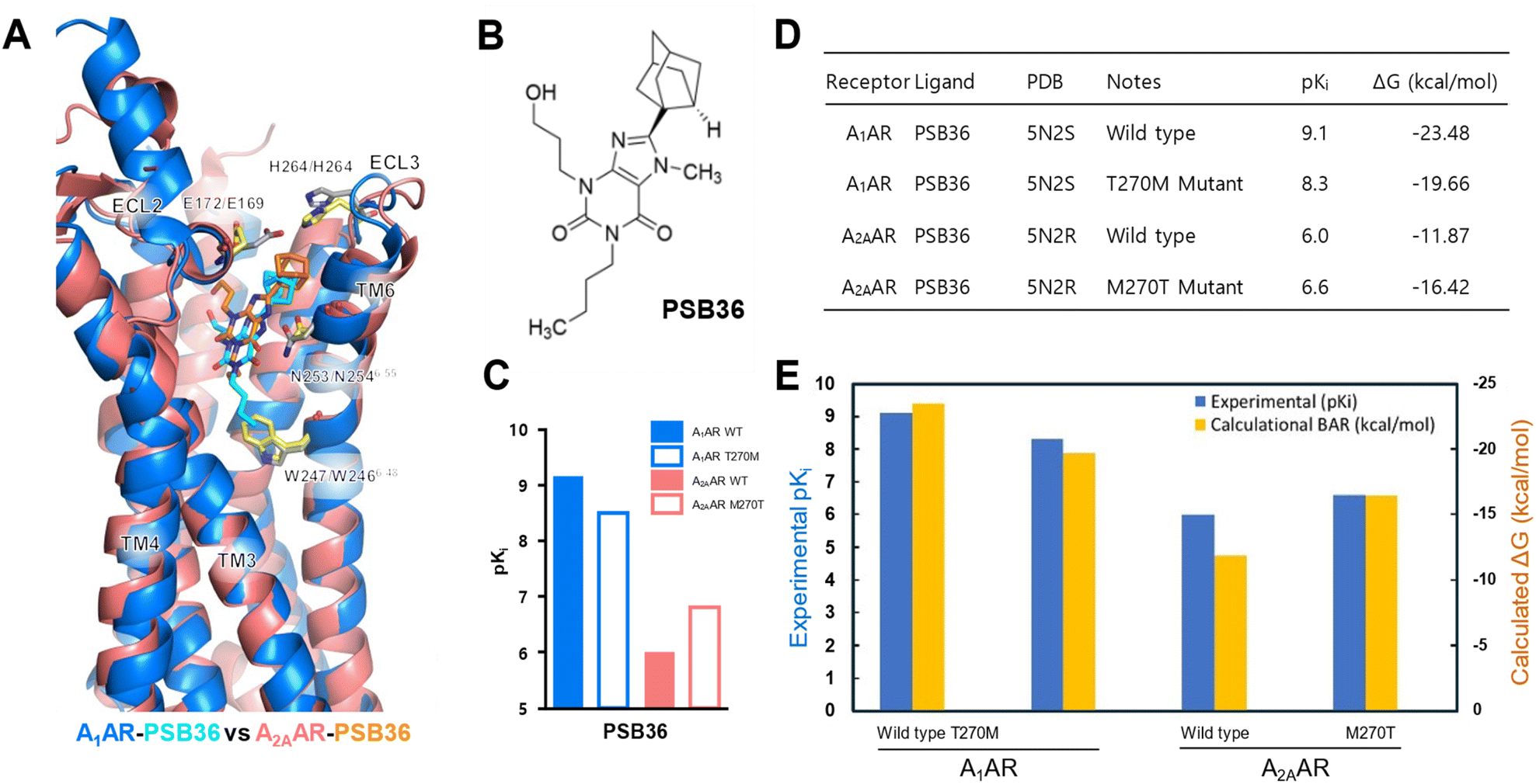

Fig. 3 Comparison of binding modes of PSB36 bound to A₁AR and A_2AAR. (A) Superposition of PSB36 bound A₁AR (blue ribbon) and A_2AAR (pink ribbon). The PSB36 ligand in A₁AR is represented with cyan carbon atoms, while the same ligand in A_2AAR is shown with orange carbon atoms. (B) 2D structure of the PSB36 used in this study. (C) Competition binding experiments for wild-type and mutated A2A and A1 receptor bound PSB36. (D)–(E) Comparison of competition binding experiments (pK_i) and binding free energies (ΔG) of the wild type and T270M (A₁AR)/M270T (A_2AAR) mutant for A₁AR and A_2AAR. In particular, a detailed comparison of experimental and computational binding affinities is presented in (E), with experimental and computational pK_i predictions highlighted in blue and yellow colors. See ESI Table S6† for numerical data on BAR binding free energies.

Binding free energy calculations were performed in this study, akin to the β₁AR case, to validate the experimental data of mutagenesis in A₁AR and A_2AAR, and the results were compared with Cheng et al.'s experimental findings (Fig. 3D and E). Experimental structures and K_i values for A₁AR and A_2AAR were obtained from ref. 34. To compare experimental and calculated correlations, experimental values were transformed into −log K_i (pK_i), and binding affinities were predicted using our BAR-based free energy scheme. As seen in Fig. 3D and E, the ligand PSB36 was analyzed to be more selective for A₁AR in both experimental and calculated values, while the selectivity for A_2AAR was predicted to be relatively low.

This is attributed to the initial orientation of the extracellular loop in both A₁AR and A_2AAR. In A_2AAR, the noradamantyl head group of PSB36 is oriented toward the extracellular face, disrupting the formation of the salt bridge between E169 and H264 (Fig. 3A). The reason is analyzed to be that, in A_2AAR, the butyl tail of PSB36 is surrounded by the hydrophobic area formed by W246^6.48 and N253^6.55, preventing it from positioning more deeply in the binding site compared to A₁AR (ESI Fig. S3A†).

To elaborate further, compared to PSB36 bound to the wild-type of A_2AAR, the same ligand in A₁AR of the wild-type sequence shows more favorable (stable) interaction energy in almost all residues, with the largest increases observed at N^6.55 and L^6.51. This can be explained by the “Velcro effect”, where the increase in the binding energy between PSB36 and A₁AR in the wild-type is thought to be the result of overall multiple small increases in the interaction energy around the ligand. In other words, the number of ligand–receptor contacts in the PSB36–A_2AAR decreases, which increases the mobility of the agonist and thus conversely decreases the binding free energy in the ligand–GPCR complex.

Lastly, regarding the effect of mutations in adenosine receptors, the methionine mutation in A₁AR (T270M) decreased the affinity, while the threonine mutation in A_2AAR (M270T) increased affinity (Fig. 3D and E). According to Cheng et al., the bulky methionine in A_2AAR, unlike threonine in A₁AR, can cause a steric clash with PSB36 in A_2AAR. This is because ECL2 in A₁AR is located perpendicular to the membrane surface, whereas, in A_2AAR, it is parallel to the membrane surface, and also, the extracellular half of TM7 in A_2AAR is moved to the binding pocket, where M270 binds the PSB ligand.

Case 3 . Selectivity of the antagonist in A1AR over that of A3AR

As mentioned in Case 2 above, natural agonists of A₁AR are gaining interest for their cardioprotective and cerebroprotective properties, and are of particular interest as a potential treatment for diabetes.^35–38 On the other hand, A₁AR antagonists have been evaluated for their beneficial roles as diuretics, antihypertensive medications or in the control of heart failure, allergy, and asthma, and may be used therapeutically.³⁹

In Case 3, molecular modeling analysis and free energy calculations were performed using SAR data⁴⁰ based on the crystal structure of human A₁AR bound to a selective antagonist (pdb code of 5UEN)⁴¹ to verify and correlate the structural features of the purine base with the experiment, which shows different binding affinities depending on its derivatives. To verify the selectivity with experimentally found A₁AR, we formed a complex of the same ligand using human A₃AR and compared it with the same MD simulations and BAR binding free energy calculation. However, since A₃AR (pdb code of 1OEA) has been removed from the current PDB entry, the structure was set up using the available AlphaFold2 predicted structure from the Uniprot website, and modeling was then performed using it.

Overall, the structure of A₁AR was adopted to crystallize in an inactive conformation, and the intracellular loop 1 (ICL1) between transmembrane helices exhibited a similar form to that of A₃AR. Compared with A₃AR, a prominent difference in shape is observed in the orientation of extracellular loop 2 (ECL2) (Fig. 4). While ECL2 of A₁AR exists perpendicularly to the membrane plane, in A₃AR, it adopts a conformation parallel to the membrane surface (Fig. 4B). This phenomenon influences the volume of the binding site, causing the transmembrane helices (TMs) in A₃AR to shift inward, reducing the overall volume. This provides a rationale for the ligand selectivity of A₁AR being dominant over A₃AR (Fig. 4C).

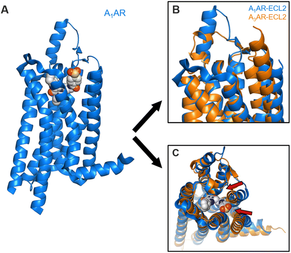Fig. 4 Comparison of ligand-binding sites in the A₁AR crystal structure and A₃AR obtained by Alphafold2 prediction. (A) Overview of the A₁AR in complex with DU172 crystal structure. (B) and (C) Superimposition of backbone ribbons of the A₁AR structure in complex with PSB36 with A₃AR structure ((B) side view, (C) extracellular view).

To validate ligand selectivity of A₁AR and A₃AR by an in silico approach, we obtained structure–activity relationship (SAR) data for both types of adenosine receptors from ref. 40, and performed BAR binding free energy calculations for A₁AR and A₃AR, respectively, and compared them with experimental K_i values. Each derivative ligand was structurally modeled in the form of a receptor–ligand complex, and binding free energies were calculated and compared with experimental values (Table 1). A set of compounds with pK_i affinities of 7.0–8.6 and 4.9–6.5 for A₁AR and A₃AR, respectively, was extracted from ref. 40, and binding free energy was calculated through MD simulations under identical conditions to investigate selectivity.

Table 1 Experimental affinity (pK_i) and calculated free energy (ΔG, kcal mol⁻¹) data for the series of purine derivatives in radioligand binding assays at human A₁AR and A₃AR⁴⁰

	R	R1	A1AR		A3AR
			pKi	ΔG	pKi	ΔG
4	Et	H	7.5	−16.1	5.2	−5.7
12	Me	H	7.6	−15.4	4.9	−3.3
13	Pr	H	7.0	−9.1	5.0	−4.9
14	Me	cButyl	8.5	−19.4	—	—
15	Et	cButyl	8.2	−17.3	—	—
16	Pr	cButyl	7.8	−17.1	—	—
17	Me	cPentyl	8.6	−19.0	—	—
18	Et	cPentyl	8.4	−20.3	6.5	−8.0
19	Pr	cPentyl	8.0	−19.4	6.1	−7.7
20	Me	3-THF	8.1	−15.8	5.2	−6.5
21	Et	3-THF	8.0	−14.7	5.8	−6.8
22	Pr	3-THF	7.6	−15.9	5.6	−6.9
23	Me	cHexyl	8.2	−18.9	—	—
24	Et	cHexyl	8.0	−17.1	—	—
25	Pr	cHexyl	7.6	−17.5	—	—
38	Ph-2-(CH3)		7.3	−12.5	—	—
39	Ph-3-(CH3)		8.2	−18.1	—	—
40	Ph-4-(CH3)		8.1	−17.7	—	—
44	Ph-4-(F)		8.2	−18.5	—	—
45	Ph-4-(OCH3)		7.8	−17.1	—	—

---

As shown in Table 1 and Fig. 5, overall, A₁AR predominantly exhibited higher experiment-to-calculation ratios, while in contrast, A₃AR had lower values in both experimental and calculated data (Fig. 5A, B and ESI Fig. S4†). For both A₁AR and A₃AR, the calculated values showed significantly higher correlation with the experimental data (R² = 0.7008 and 0.809). In these cases, the 18th and 19th derivatives exhibited the highest binding affinities toward A₁AR and A₃AR targets with a relative difference of approximately 1 kcal mol⁻¹ between them through experimental and computational validations, which was revealed to have a strong hydrogen bond between the purine of the ligand and N^6.55 through structural analysis. Additionally, the hydrophobic binding site of A₁AR and A₃AR is commonly linked by F171^ECL2/F168^ECL2 and I274^7.39/L268^7.39. However, unlike A₃AR, A₁AR is more strongly connected to the ligand, primarily due to the additional hydrophobic contributions of V87^3.32 and L250^6.51.

Fig. 5 Molecular basis of adenosine receptors and binding free energy calculations in A₁AR and A₃AR. (A) and (B) Correlation between calculated binding free energies of A₁AR (A) and A₃AR ligands (B) and experimental K_i values. The coefficient of determination (R²) is shown in the figures as red. (C) and (D) Representative binding mode structures of the adenosine receptors bound to #18 in A₁AR (C) and A₃AR (D). See Table 1 for numerical data on BAR binding free energies.

The difference in the relative binding affinity of the 18th derivatives with the best scores at A₁AR and A₃AR (−20.3 and −8.0 kcal mol⁻¹) was also observed through the movement of each ligand (ESI Fig. S4†). In the same way as in Case 1, we evaluated the movement of the nitrogen atoms in the ligand over the entire MD trajectory. Our analysis showed that the ligand in A₁AR was less movable than that in A₃AR, and concluded that it had stronger contacts in A₁AR and in A₃AR at the orthosteric binding site, contributing to its superior binding affinity.

Case 4. Effect of salt bridge interaction on the binding affinity

A_2AAR is recognized as a promising target in a wide range of diseases, including ADHD (attention deficit hyperactivity disorder) and Parkinson's disease.^42–45 Antagonism of A_2AAR is known to play a crucial role in immunotherapeutic treatment for cancer.⁴⁶ In recent studies on A_2AAR, prominent features influencing the dissociation of the representative antagonist ZMA241835 (ZMA) have been identified.⁴⁷ One notable feature is the salt bridge formed between E169 in extracellular loop 2 (ECL2) between TM4 and TM5, and H264 in extracellular loop 3 (ECL3) between TM6 and TM7. The significance of the salt bridge is based on the residence time of the ligand in the binding site, which is also involved in the energy of the ligand and target at the binding site. In other words, mutation of either residue to break the salt bridge increases the dissociation rate of the ligand, which has a significant impact on the conservation of energy measurable in silico.

In this study, we observed the effect of salt bridges on the A_2AAR using 10 SAR compounds from the ref. 48 including two ZMA-bound crystal structures (pdb of 3PWH and 3EML) by performing MD simulations followed by BAR binding free energy. As shown in Fig. 6A, ZMA bound to thermostabilized A_2AAR (pdb code of 3PWH) contains a total of six single mutations (A54L^2.52, K122A^4.43, V239A^6.41, R107A^3.55, L202A^5.63, L235A^6.37) that resulted in salt bridge disruption, whereas the A_2AAR structure crystallized in the wild-type sequences (pdb code of 3EML) with the formation of a stable and rigid salt bridge.

Fig. 6 Evaluation of the H264–E169 salt bridge using molecular dynamics followed by binding free energy calculation. (A) Difference in the orthosteric site accessibility between the A_2AAR crystal structure bound to ZMA and a SAR structure (25d) used in this study for BAR free energy calculation. The SAR structure (25d) with the salt bridge formed and a 3PWH crystal structure without a salt bridge were colored in cyan and magenta, respectively. (B) Measurement of the minimum distance between the nitrogen atoms in the sidechain of H264 and the oxygen atoms in the sidechain of E169 for all SAR data. (C) Comparison of experimental binding affinity (K_i) with calculated BAR binding free energy results from the SAR data used, and relative energy stabilities (ΔΔG) from the 25d compound. (D) Linear correlation between experimental pK_i and calculated binding free energy ΔG for a total of 9 SAR data.

The MD simulations starting from the thermostabilized A_2AAR crystal structures bound to ZMA (pdb code of 3PWH) (Fig. 6A and B) show that the salt bridges are broken and the binding free energy was unstable (ΔG = −11.8 kcal mol⁻¹), while another crystal structure from the wild-type sequence of A_2AAR bound to ZMA (pdb code of 3EML) and a 25d complex with lower energies exhibited long-lasting salt bridges. Especially, for the ZMA-bound complex structure in the wild-type sequence, the stability of the salt bridge was predicted to be −35 kcal mol⁻¹ in enthalpic contribution, whereas the complex with the next most energetically stable compound 25d decreased in strength by 3 kcal mol⁻¹ (−32 kcal mol⁻¹ of enthalpic contribution) (see ESI Fig. S5† for the whole information). The other derivatives such as 25b and 25c derivatives also demonstrated 31–33 kcal mol⁻¹ of enthalpic energy increase and a corresponding increase in the strength of the salt bridge compared to ZMA-bound thermostabilized A_2AAR. Moreover, there is a substantial correlation between experimentally proven pK_i values and calculated binding free energy (R² = 0.7824 and MUE = 1.87) (Fig. 6C and D). In general, this shows that binding free energy predictions using the in silico BAR algorithm can be utilized for experimental validation of unknown (new) derivatives for GPCR targets.

As a complement to ligand binding affinity, we examined the contribution of volume differences to ligand movement and flexibility through changes in the average volume of the ligand binding site obtained from the overall MD simulations (ESI Fig. S6†). Our results show that the average volume of the ZMA ligand in the wild-type, 25d, and 11 derivatives remains similar in A_2AAR, but there is a significant increase in the volume of 25a and 25e bound A_2AAR. Although the correlation between the volume of the orthosteric binding site and the degree of ligand mobility with the binding free energy cannot be answered, it has been observed that the volume of ligands is reduced in compounds with strong binding affinity.

Conclusions

As discussed by Mobley and Klimovic, unreliable binding free energy predictions can have a significant impact on even low-level drug discovery campaigns.⁴⁹ With the current advances in computational power, the alchemical free energy calculation has gained much attention as a non-empirical tool for predicting and understanding protein–ligand binding. However, current prediction tools still face many challenges, such as difficulties in adequate sampling and incomplete knowledge of the force field. The reality is that multiple tests are still required in special cases, such as when an isolated charged mono-atomic molecule is contained in a ligand binding site or in charged thermostabilized mutants. However, assuming that hardware and algorithmic performance for free energy calculations continue to improve, accurate rescoring methods may be used to develop leads for GPCR targets in the long term. It is known that for large but fairly rigid systems such as GPCRs, molecular dynamics based free energy calculations show RMS errors in excess of 2 kcal mol⁻¹ when starting from the docking structure, but can be reduced to as low as 0.8 kcal mol⁻¹ when starting from crystal structure. This shows the limitations of current docking techniques, but also indicates that the accuracy of the docking pose is an important factor in predicting binding affinity.

In this study, we demonstrated the efficiency of a BAR-based binding affinity prediction method by calculating the functional activity of different types of ligands, including the selective antagonist/agonist, mutation effect, and salt bridge effect of GPCRs based on X-ray crystal structures and verifying them through free energy calculations. Whereas previous free energy calculation methods have provided a one-off basis approach to GPCR studies, this study investigated four different cases of different types of GPCR targets. Our results show how accurate binding energy predictions are consistent with in vitro assay results, which could be valuable for GPCR drug discovery.

This study also demonstrates the potential of BAR-based free energy calculations for GPCR target applications. To the best of our knowledge, this is the first study of a BAR-based free energy calculation method that takes into account a variety of drug-like molecules and biologically relevant GPCR targets currently under investigation for their therapeutic potential. Through our work, we illustrated that BAR free energy calculations based on a TI-mixed FEP approach yield binding free energies that are equivalent or superior to Hamiltonian replica exchange methods and other equilibrium FEP approaches.

We applied BAR free energy to all four cases: four agonists binding to inactive and active β₁AR, wild-type and mutants of A1/A2A adenosine receptors, an antagonist selective for A₁AR over A₃AR, and an A_2AAR antagonist affecting salt bridge strength. Our results demonstrate the potential of MD simulations to efficiently estimate ligand–GPCR binding affinity and pave the way for further exploration of BAR-based binding free energy approaches. In conclusion, this study provides evidence that the absolute binding free energy of a protein–ligand can be accurately predicted by alchemical calculations.

While molecular docking has been widely used for initial hit identification, its ability to accurately predict binding affinity remains limited due to inherent simplifications in scoring functions and rigid-body assumptions. To address this limitation, molecular dynamics-based alchemical binding free energy methods—particularly the BAR (Bennett Acceptance Ratio) algorithm—have increasingly been employed as a follow-up approach to refine docking results and prioritize hits with higher computational and experimental confidence as seen in many alchemical BAR free energy studies on GPCR targets.^50–53 Our MIND-BAR alchemical approach enables thorough sampling of the relevant conformational landscape required for accurate predictions, making it particularly well-suited for flexible binding pockets such as those found in GPCRs. During the MD equilibration step, which serves as a preprocessing phase for binding affinity prediction, position and distance restraints were carefully applied to minimize ligand displacement and structural deviations, thereby improving ligand stability. Furthermore, to increase the reliability of the binding affinity estimates, five independent production runs were performed using different random seeds. This allowed for diverse sampling, and the most frequently observed binding free energy values were selected as the final result, thereby enhancing correlation with experimental data.

Our MIND-BAR protocol significantly reduces the variability in binding free energy estimates compared to conventional computational approaches, providing more robust and reproducible results. In particular, by incorporating both forward and backward perturbation data, it markedly enhances statistical reliability by decreasing the variance of computed ΔG values relative to traditional one-way FEP methods. Furthermore, through the use of inequivalent λ-scaling—adding more finely spaced λ values in regions with poor overlap and steep free energy changes, and using wider spacing in more stable regions—we improve both the accuracy and efficiency of binding affinity predictions. This approach offers a critical advantage when dealing with complex molecular systems such as GPCRs. These methods not only improve the reliability of in silico screening but also serve as powerful tools in the lead optimization stage of drug design, providing quantitative insights for rational compound selection and guiding the design of subsequent experimental studies.

Materials and methods

Theory

As mentioned earlier, various chemical free energy calculation algorithms are currently employed to predict the binding affinities between targets and ligands. Binding free energy calculation algorithms are commonly divided into two main approaches (Thermodynamic Integration (TI) and Free Energy Perturbation (FEP)) and current research is actively exploring combinations of these methods for improved efficacy. In TI, the free energy change along a path composed of states from initial to final (1 to K states) is calculated as the weighted sum of ensemble averages of derivatives of the potential energy function with respect to the coupling parameter λ.

In the above equation, W_i represents the weight coefficients that vary depending on the integration method used, and in practical numerical integration for TI, it can be expressed in various ways. Various TI methods exhibit differences in performance based on the integration of the ∂U/∂λ curve, ultimately depending on the chosen alchemical path.

The BAR method applied in this study incorporates various techniques associated with perturbation-based binding free energy algorithms, but fundamentally relies on the modified BAR algorithm proposed by Paliwal–Shirts,⁸ as represented by the equation below. Currently, there is a lack of universally recognized or widely known conventional names, such as BAR and multi-state BAR (referred to as mBAR).

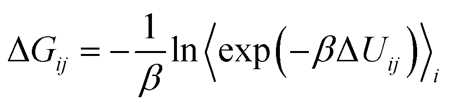
Methods directly based on the Zwanzig relationship⁵⁴ generally exhibit different free energy differences in the forward and backward directions, and this discrepancy is attributed to the bias in ΔU_ij due to insufficient sampling. Our BAR algorithm minimizes bias in ΔG by simultaneously considering both forward ΔU_ij and backward ΔU_ij during post-processing.

where .

A BAR-based free energy program has an advantage in that it does not need to retain all potential energy differences for post-processing. It accumulates averages of forward and backward reactions during simulation, designed to compute the free energy change between adjacent states with minimal variance based on the collected data for each corresponding state pair (ESI Fig. S1†). This is considered to be a similar approach to the Weighted Histogram Analysis Method (WHAM)^55,56 designed with a histogram width of 0.

The accuracy of TI is unrelated to the overlap of the energy distribution but is determined by the mean curvature function, 〈(∂2U)/(∂λ)²〉. Free energy perturbation (FEP) also has technical limitations as it depends on the overlap of energy representation sampling rather than the smoothness of integration. To overcome these limitations of FEP, the BAR-based algorithm has performed multiple MD simulations with diverse random seeds before energy analysis to solve the lack of sampling. Also, an algorithm was implemented to minimize the free energy discrepancy between the forward/backward directions by inequivalent scaling factors (see the MD simulation parameter).

Target preparation and system setup

In this study, a total of 4 case studies were prepared for GPCR targets and summarized in ESI Table S4.† First, the initial target structure was obtained from the Protein Data Bank (http://www.rcsb.org). The overall target preparation utilized the protein preparation functionality, a part of the in-house platform module called MIND (Modeling with Intelligence for Novel Drug), consistently. All solvent water present in the crystal structure was excluded from the calculations, and protonation states were assigned at pH 7.0. Generally, thermostabilized mutant GPCRs were prepared by back-mutating to the wild-type sequence. For the A₃AR protein in Case 3, which was missing from the PDB entry, the Alphafold2 (ref. 47, 57 and 58) structure was selected as the initial structure for modeling.

MD simulation parameter

The simulation parameters used in this study were employed following the same methodology as previous GPCR research publicly available. The protein–ligand complexes for all cases, as well as the setup for the T270M/A₁AR and M270T/A_2AAR mutants in Case 2, were generated using our in-house MIND mutation tool. The setup for all proteins utilized the CHARMM36 force field,⁵⁹ while the force field for ligands was determined using Antechamber.^60,61 For the bilayer embedding around the proteins, a POPC (1-palmitoyl-2-oleoyl-sn-glycero-3-phosphocholine) bilayer was employed, and the water model used was TIP3P.⁶² To neutralize the system, Na⁺ and Cl⁻ ions were added to achieve a salt concentration of 0.15 M. Stabilization of the entire system was achieved by utilizing the relaxation and equilibration processes provided by our MIND platform to perform system minimization and equilibration.

The entire system was minimized using the steepest descent method in the GROMACS package.²¹ Each solvated GPCR complex was first equilibrated by the NVT ensemble until 200 ps at 300 K. During equilibration, protein and ligand were subjected to stepwise reducing position restraints from 5 to 1 kcal mol⁻¹ under the conditions of constant temperature and pressure (NPT). In the final equilibration step, all restraints were released to facilitate the equilibration of the entire system. The final snapshot of the equilibration step was used for the starting structure of production simulations. The production phase of MD simulations employed the Parrinello–Rahman barostat⁶³ with a temperature of 300 K and a pressure of 1 bar. The SETTLE⁶⁴ and LINCS algorithms⁶⁵ were used for the bond and angle for water and all other bonds with a 2 fs integration time step. After the relaxation and equilibration of all systems, we conducted the production simulation for 50 ns. All five replica runs were executed with different velocities, and only three replicas excluding the two with significant deviations were used as the initial structures for BAR-based binding free energy calculations. During the simulation, a cutoff radius of 12 Å was employed for van der Waals and electrostatic interactions, and particle mesh Ewald (PME)⁶⁶ was utilized for long-range electrostatic interactions.

BAR-based free energy procedure

For all binding free energy calculations, a total of 38 NVidia RTX GPU cores were employed. For the final free energy calculation, our BAR-based algorithm utilized the basic algorithm of BAR (Bennett Acceptance Ratio)^8,67–69 that typically combines information from forward and backward free energy perturbation directions. We specified a total of 25 inequivalent scaling factor (λ) values (0.025, 0.05, 0.075, 0.1, 0.125, 0.15, 0.2, 0.25, 0.3, 0.35, 0.4, 0.45, 0.5, 0.55, 0.6, 0.65, 0.7, 0.75, 0.8, 0.85, 0.9, 0.925, 0.95, 0.975, and 1) to smoothly pass the free energy convergence for each lambda in the bi-directional pathway (ESI Fig. S1†). The λ schedule was explicitly using the ‘fep-lambdas’ directive. Separate λ vectors were for coulombic decoupling (electrostatics) and Lennard–Jones decoupling (van der Waals interactions) to enhance sampling efficiency and avoid strong end-point artifacts. In all of the BAR calculations for all GPCRs, electrostatic and van der Waals interactions were treated as soft core, as described by Beutler et al.⁷⁰ Soft-core parameters were set as follows: sc-alpha = 0.5, sc-power = 1, sc-sigma = 0.3 and sc-coul = yes. The LINCS⁶⁵ bond restraining order was set to 12 (lincs_order = 12), with a cutoff-based PME elestrostatics scheme. All GPCR systems were simulated in the NPT ensemble at 301 K and 1 bar, using a V-rescale thermostat and a Parrinello–Rahman barostat. The ligand to be decoupled was defined by ‘couple-moltype = LIG’, and intra-ligand interactions were excluded via ‘couple-intramol = no’. This setup ensured that only inter-molecular interactions between solute and solvent were subject to alchemical scaling. All energy analyses were carried out using the GROMACS bar module,²¹ and throughout the simulation processes, basic analyses such as RMSD (root mean square deviation) and RMSF (root mean square fluctuation) were monitored for the measurement of protein stability, and all target proteins exhibited Cα-RMSD values of 3.0 Å or less. Correlation plots were presented for all analyses of binding free energy, with an emphasis on correlation coefficients (R or R²), MUE (mean unsigned error), and RMSE (root mean square error).

All methods and description for analyses regarding classical molecular dynamics for GPCRs and alchemical binding free energy were introduced in the ESI.† All the representative structures shown in all figures were rendered using PyMOL⁷¹ and VMD.⁷² All the analyses reported here from the atomistic MD simulation trajectories were done using the 5 × 50 ns ensemble collected from the last 30 ns of each of 5 simulations for each system.

Data availability

The data supporting this article have been included as part of the ESI.†

Author contributions

Minkyu Kim: software; investigation; formal analysis; data curation; writing – original draft; writing – review & editing. Jian Jeong: software; investigation; data curation. Donghwan Kim: software; investigation; formal analysis; writing – original draft. Sangbae Lee: conceptualization; methodology; software; investigation; writing – review & editing; supervision; project administration. Art E. Cho: conceptualization; methodology; supervision; funding acquisition.

Conflicts of interest

The authors declare the following competing financial interest(s): A. E. C. has a significant financial stake in and is the Founder and CEO of inCerebro Co., Ltd. Additionally, D. K. and S. L. were formerly affiliated with inCerebro and are now affiliated with Atomatrix. Contact: E-mail: donghwanz@atomatrix.co.kr; and sblee@atomatrix.co.kr.

Acknowledgements

This work was supported by a National Research Foundation of Korea grant funded by the Korean government's Ministry of Science and Information Technology (grant no. RS-2021-NR060107, RS-2023-00227084, and RS-2024-00404854). The authors also thank Molsis, Inc. and Chemical Computing Group for their generosity in providing MOE software, which was used in part of their work.

Notes and references

1. W. E. Miranda, S. Y. Noskov and P. A. Valiente, J. Chem. Inf. Model., 2015, 55, 1867–1877.
2. S. Genheden and U. Ryde, Expert Opin. Drug Discov., 2015, 10, 449–461.
3. R. Kumari, R. Kumar, Open Source Drug Discovery Consortium and A. Lynn, J. Chem. Inf. Model., 2014, 54, 1951–1962.
4. R. W. Zwanzig, J. Chem. Phys., 1954, 22, 1420–1426.
5. D. L. Beveridge and F. M. DiCapua, Annu. Rev. Biophys. Biophys. Chem., 1989, 18, 431–492.
6. M. Lawrenz, J. Wereszczynski, J. M. Ortiz-Sánchez, S. E. Nichols and J. A. McCammon, J. Comput.-Aided Mol. Des., 2012, 26, 569–576.
7. T. Steinbrecher, I. S. Joung and D. A. Case, J. Comput. Chem., 2011, 32, 3253–3263.
8. M. R. Shirts, E. Bair, G. Hooker and V. S. Pande, Phys. Rev. Lett., 2003, 91, 140601.
9. C. H. Bennett, J. Comput. Phys., 1976, 22, 245–268.
10. I. Kim and T. W. Allen, J. Chem. Phys., 2012, 136, 164103.
11. T. J. Giese and D. M. York, J. Chem. Theory Comput., 2019, 15, 5543–5562.
12. A. Laio and M. Parrinello, Proc. Natl. Acad. Sci. U. S. A., 2002, 99, 12562–12566.
13. H. S. Hansen and P. H. Hünenberger, J. Comput. Chem., 2010, 31, 1–23.
14. M. Kaukonen, P. Söderhjelm, J. Heimdal and U. Ryde, J. Phys. Chem. B, 2008, 112, 12537–12548.
15. X. Chen, X. Zhao, Y. Xiong, J. Liu and C.-G. Zhan, J. Phys. Chem. B, 2011, 115, 12208–12219.
16. H. Lu, X. Huang, M. D. M. AbdulHameed and C.-G. Zhan, Bioorg. Med. Chem., 2014, 22, 2149–2156.
17. P. Santos-Otte, H. Leysen, J. van Gastel, J. O. Hendrickx, B. Martin and S. Maudsley, Comput. Struct. Biotechnol. J., 2019, 17, 1265–1277.
18. A. S. Hauser, S. Chavali, I. Masuho, L. J. Jahn, K. A. Martemyanov, D. E. Gloriam and M. M. Babu, Cell, 2018, 172, 41–54.
19. T. Schöneberg and I. Liebscher, Pharmacol. Rev., 2021, 73, 89–119.
20. S. Guo, T. Zhao, Y. Yun and X. Xie, Am. J. Physiol.: Cell Physiol., 2022, 323, C583–C594.
21. M. J. Abraham, T. Murtola, R. Schulz, S. Páll, J. C. Smith, B. Hess and E. Lindahl, SoftwareX, 2015, 1–2, 19–25.
22. B. R. Brooks, C. L. Brooks III, A. D. Mackerell Jr, L. Nilsson, R. J. Petrella, B. Roux, Y. Won, G. Archontis, C. Bartels, S. Boresch, A. Caflisch, L. Caves, Q. Cui, A. R. Dinner, M. Feig, S. Fischer, J. Gao, M. Hodoscek, W. Im, K. Kuczera, T. Lazaridis, J. Ma, V. Ovchinnikov, E. Paci, R. W. Pastor, C. B. Post, J. Z. Pu, M. Schaefer, B. Tidor, R. M. Venable, H. L. Woodcock, X. Wu, W. Yang, D. M. York and M. Karplus, J. Comput. Chem., 2009, 30, 1545–1614.
23. D. A. Case, T. E. Cheatham III, T. Darden, H. Gohlke, R. Luo, K. M. Merz Jr, A. Onufriev, C. Simmerling, B. Wang and R. J. Woods, J. Comput. Chem., 2005, 26, 1668–1688.
24. U. Gether, Endocr. Rev., 2000, 21, 90–113.
25. D. M. Rosenbaum, S. G. F. Rasmussen and B. K. Kobilka, Nature, 2009, 459, 356–363.
26. G. Vauquelin and I. Van Liefde, Fundam. Clin. Pharmacol., 2005, 19, 45–56.
27. G. G. Gregorio, M. Masureel, D. Hilger, D. S. Terry, M. Juette, H. Zhao, Z. Zhou, J. M. Perez-Aguilar, M. Hauge, S. Mathiasen, J. A. Javitch, H. Weinstein, B. K. Kobilka and S. C. Blanchard, Nature, 2017, 547, 68–73.
28. X. J. Yao, G. Vélez Ruiz, M. R. Whorton, S. G. F. Rasmussen, B. T. DeVree, X. Deupi, R. K. Sunahara and B. Kobilka, Proc. Natl. Acad. Sci. U. S. A., 2009, 106, 9501–9506.
29. A. Manglik, T. H. Kim, M. Masureel, C. Altenbach, Z. Yang, D. Hilger, M. T. Lerch, T. S. Kobilka, F. S. Thian, W. L. Hubbell, R. S. Prosser and B. K. Kobilka, Cell, 2015, 161, 1101–1111.
30. L. Ye, N. Van Eps, M. Zimmer, O. P. Ernst and R. S. Prosser, Nature, 2016, 533, 265–268.
31. S. M. Foord, T. I. Bonner, R. R. Neubig, E. M. Rosser, J. P. Pin, A. P. Davenport, M. Spedding and A. J. Harmar, Pharmacol. Rev., 2005, 57, 279–288.
32. T. Warne, P. C. Edwards, A. S. Doré, A. G. W. Leslie and C. G. Tate, Science, 2019, 364, 775–778.
33. S. Sheth, R. Brito, D. Mukherjea, L. P. Rybak and V. Ramkumar, Int. J. Mol. Sci., 2014, 15, 2024–2052.
34. R. K. Y. Cheng, E. Segala, N. Robertson, F. Deflorian, A. S. Doré, J. C. Errey, C. Fiez-Vandal, F. H. Marshall and R. M. Cooke, Structure, 2017, 25, 1275–1285.
35. R. R. Morrison, B. Teng, P. J. Oldenburg, L. C. Katwa, J. B. Schnermann and S. J. Mustafa, Am. J. Physiol.: Heart Circ. Physiol., 2006, 291, H1875–H1882.
36. L. Ruan, G. Li, W. Zhao, H. Meng, Q. Zheng and J. Wang, Antioxidants, 2021, 10, 1112.
37. A. K. Dhalla, J. W. Chisholm, G. M. Reaven and L. Belardinelli, in Adenosine Receptors in Health and Disease, ed. C. N. Wilson and S. J. Mustafa, Springer, Berlin, 2009, ch. 9, pp. 271–295.
38. R. Faulhaber-Walter, W. Jou, D. Mizel, L. Li, J. Zhang, S. M. Kim, Y. Huang, M. Chen, J. P. Briggs, O. Gavrilova and J. B. Schnermann, Diabetes, 2011, 60, 2578–2587.
39. C. N. Wilson, Br. J. Pharmacol., 2008, 155, 475–486.
40. C. Lambertucci, G. Marucci, D. Dal Ben, M. Buccioni, A. Spinaci, S. Kachler, K.-N. Klotz and R. Volpini, Eur. J. Med. Chem., 2018, 151, 199–213.
41. A. S. Doré, N. Robertson, J. C. Errey, I. Ng, K. Hollenstein, B. Tehan, E. Hurrell, K. Bennett, M. Congreve, F. Magnani, C. G. Tate, M. Weir and F. H. Marshall, Structure, 2011, 19, 1283–1293.
42. P. J. Richardson, H. Kase and P. G. Jenner, Trends Pharmacol. Sci., 1997, 18, 338–344.
43. J. Burgueño, R. Franco and F. Ciruela, in Antidepressants, Antipsychotics, Anxiolytics, ed. H. Buschmann, J. L. Díaz, J. Holenz, A. Párraga, A. Torrens and J. M. Vela, Wiley-VCH, Weinheim, 2007, pp. 1090–1182.
44. J. Biederman and S. V. Faraone, Lancet, 2005, 366, 237–248.
45. S. V. Faraone, R. H. Perlis, A. E. Doyle, J. W. Smoller, J. J. Goralnick, M. A. Holmgren and P. Sklar, Biol. Psychiatry, 2005, 57, 1313–1323.
46. F. Yu, C. Zhu, Q. Xie and Y. Wang, J. Med. Chem., 2020, 63, 12196–12212.
47. J. Jumper, R. Evans, A. Pritzel, T. Green, M. Figurnov, O. Ronneberger, K. Tunyasuvunakool, R. Bates, A. Žídek, A. Potapenko, A. Bridgland, C. Meyer, S. A. A. Kohl, A. J. Ballard, A. Cowie, B. Romera-Paredes, S. Nikolov, R. Jain, J. Adler, T. Back, S. Petersen, D. Reiman, E. Clancy, M. Zielinski, M. Steinegger, M. Pacholska, T. Berghammer, S. Bodenstein, D. Silver, O. Vinyals, A. W. Senior, K. Kavukcuoglu, P. Kohli and D. Hassabis, Nature, 2021, 596, 583–589.
48. P. Minetti, M. O. Tinti, P. Carminati, M. Castorina, M. A. Di Cesare, S. Di Serio, G. Gallo, O. Ghirardi, F. Giorgi, L. Giorgi, G. Piersanti, F. Bartoccini and G. Tarzia, J. Med. Chem., 2005, 48, 6887–6896.
49. D. L. Mobley and P. V. Klimovich, J. Chem. Phys., 2012, 137, 230901.
50. A. F. Marmolejo-Valencia and K. Martínez-Mayorga, J. Comput.-Aided Mol. Des., 2017, 31, 467–482.
51. A. F. Marmolejo-Valencia, A. Madariaga-Mazón and K. Martinez-Mayorga, SN Appl. Sci., 2021, 3, 566.
52. M. Javanainen, G. Enkavi, R. Guixà-González, W. Kulig, H. Martinez-Seara, I. Levental and I. Vattulainen, PLoS Comput. Biol., 2019, 15, e1007033.
53. K. Georgiou, A. Konstantinidi, J. Hutterer, K. Freudenberger, F. Kolarov, G. Lambrinidis, I. Stylianakis, M. Stampelou, G. Gauglitz and A. Kolocouris, Biochim. Biophys. Acta, Biomembr., 2024, 1866, 184258.
54. R. W. Zwanzig, J. Chem. Phys., 1954, 22, 1420–1426.
55. A. M. Ferrenberg and R. H. Swendsen, Phys. Rev. Lett., 1989, 63, 1195–1198.
56. S. Kumar, D. Bouzida, R. H. Swendsen, P. A. Kollman and J. M. Rosenberg, J. Comput. Chem., 1992, 13, 1011–1021.
57. L. M. F. Bertoline, A. N. Lima, J. E. Krieger and S. K. Teixeira, Frontiers in Bioinformatics, 2023, 3, 1120370.
58. P. Bryant, G. Pozzati and A. Elofsson, Nat. Commun., 2022, 13, 1265.
59. J. Huang, S. Rauscher, G. Nawrocki, T. Ran, M. Feig, B. L. de Groot, H. Grubmüller and A. D. MacKerell Jr, Nat. Methods, 2017, 14, 71–73.
60. J. Wang, R. M. Wolf, J. W. Caldwell, P. A. Kollman and D. A. Case, J. Comput. Chem., 2004, 25, 1157–1174.
61. J. Wang, W. Wang, P. A. Kollman and D. A. Case, J. Mol. Graphics Modell., 2006, 25, 247.
62. P. Mark and L. Nilsson, J. Phys. Chem. A, 2001, 105, 9954–9960.
63. S. Melchionna, G. Ciccotti and B. L. Holian, Mol. Phys., 1993, 78, 533–544.
64. S. Miyamoto and P. A. Kollman, J. Comput. Chem., 1992, 13, 952–962.
65. B. Hess, H. Bekker, H. J. C. Berendsen and J. G. E. M. Fraaije, J. Comput. Chem., 1997, 18, 1463–1472.
66. U. Essmann, L. Perera, M. L. Berkowitz, T. Darden, H. Lee and L. G. Pedersen, J. Chem. Phys., 1995, 103, 8577–8593.
67. C. H. Bennett, Efficient Estimation of Free Energy Differences from Monte Carlo Data, 1976, vol. 22.
68. I. Kim and T. W. Allen, J. Chem. Phys., 2012, 136, 164103.
69. T. J. Giese and D. M. York, J. Chem. Theory Comput., 2019, 15, 5543–5562.
70. T. C. Beutler, A. E. Mark, R. C. van Schaik, P. R. Gerber and W. F. van Gunsteren, Chem. Phys. Lett., 1994, 222, 529–539.
71. The PyMOL Molecular Graphics System, Version 2.6, Schrödinger, LLC.
72. W. Humphrey, A. Dalke and K. Schulten, VMD – Visual Molecular Dynamics, J. Mol. Graphics, 1996, 14, 33–38.

---

Footnote

† Electronic supplementary information (ESI) available. See DOI: https://doi.org/10.1039/d5sc01030f

---