Calculation of proton transmembrane-electrostatic interaction force and elucidation of the water droplet experiment with a transient protonic front

Abstract

The “transmembrane-electrostatically localized proton(s)/cation(s) charge(s) (TELC(s), also known as TELP(s)) model” may serve as a theoretical framework to explain protonic cell energetics including both delocalized and localized protonic couplings. TELCs are held by their corresponding transmembrane-electrostatically localized hydroxides anions (TELAs) across the membrane through mutual transmembrane-electrostatic attractive force, which is now calculated to be in the range from 1.96 × 10⁻¹¹ to 2.28 × 10⁻¹¹ newtons (N) across a 2.5 nm thick membrane in a range of transmembrane potential from 10 to 200 mV. At a moderate transmembrane potential (100 mV), the protonic transmembrane attractive force is now calculated to be 2.08 × 10⁻¹¹ N. Accordingly, to move such a localized proton away from the membrane–liquid interface by 1 nm, it would require 1.62 × 10⁻²⁰ J of energy, which is equivalent to 3.8 times as much as the Boltzmann kT thermal kinetic energy at a physiological temperature of 37 °C, indicating that a TELCs–membrane–TELAs capacitor can be quite stable. Thus, TELCs (TELPs) formation does not require any potential barrier in liquid phases. The Zhang et al. 2012 experiment is likely to involve a transient “protonic front” effect in a single water droplet system which has no membrane and no TELPs. The use of the “Bjerrum length” approach for merely a single pair of charges (Knyazev et al., Biomolecules, 2023, 13, 1641) could underestimate the protonic transmembrane attractive force. Future TELPs research is encouraged on cell systems that should have transmembrane potential associated with certain TELCs-membrane-TELAs capacitors having excess positive charges on one side of the membrane and excess anions on the other side.

---

1. Introduction

The recently developed transmembrane-electrostatically localized proton(s)/cation(s) charge(s) (TELC(s)) model^1–3 provides a theoretical framework that can help explain protonic cell energetics including many experimental observations and elucidate bioenergetic systems including both delocalized and localized protonic couplings.^4–6 The term TELCs represent the “total transmembrane-electrostatically localized positive charges” including the charges of both the transmembrane-electrostatically localized proton(s) (TELP(s)) and the associated transmembrane-electrostatically localized non-proton cations after the proton–cation exchanging process reaching equilibrium. TELCs are immediately related to transmembrane potential that is now known as a function of TELCs population density within a TELCs-membrane-anions capacitor.^1,6 Consequently, the excess positive charges of TELCs at one side of the membrane are balanced by the excess negative charges of transmembrane-electrostatically localized hydroxides anions (TELAs) at the other side of the membrane. The formation of TELCs-membrane-TELAs capacitors has been experimentally demonstrated using a biomimetic anode water-Teflon membrane-water cathode system^7–9 through two PhD thesis research projects.^10,11

The TELCs (TELPs) model,^1–3 which may represent a complementary development to Mitchell's chemiosmotic theory, is highly useful in helping to elucidate real-world bioenergetic systems with both delocalized and localized protonic coupling. For instance, the TELPs model has been successfully employed in elucidating the decades-longstanding energetic conundrum^12–14 of ATP synthesis in alkalophilic bacteria^5,15–19 and in bettering the understanding of energetics in mitochondria.^2,3 Its application has recently led to the discovery of the TELPs “thermotrophic function” as the “Type-B energetic process”^20–24 which can isothermally utilize environmental heat energy to do useful work in helping drive the synthesis of ATP.^3,25

As discussed in a recent review article,⁹ protonic (TELPs) membrane capacitors have been experimentally demonstrated well beyond any reasonable doubt; and certain scientists such as Prof. Lan Guan as a special Collection editor for the Nature research journal Scientific Reports can well understand and appreciate the TELPs theory. In the journal editorial,²⁶ Prof. Guan as the editor clearly acknowledged that the progresses of TELPs research “refined and improved our knowledge of transport bioenergetics” including the discovery of the TELPs thermotrophic feature. Her editorial²⁶ states: “Recently, these transmembrane-electrostatically localized protons (TELPs) have been recognized as a primary contributor to Mitchell's PMF.² In addition, a follow-up study in this Collection identified a significant thermotropic component of PMF.³ Lee found that mitochondria can isothermally utilize environmental heat through TELPs to drive the synthesis of ATP, thus locking substantial amounts of the heat energy into ATP molecules. This work has refined and improved our knowledge of transport bioenergetics.

Notably, more independent researchers have started to recognize the value of the TELPs theory in their publications.^26–30 For example, the TELPs model has now been successfully employed in an excellent elucidation of their independent experimental observations³¹ including the “unexpected result” in a cellular membrane ion transport protein complex (melibiose transporter MelB)³² that could not be explained by any other existing models and/or theories.

Furthermore, through studies^6,33 based on the TELCs model, the physical origin of neural resting and action potential has better been elucidated as the voltage contributed by TELCs in a neuron “localized protons/cations–membrane–anions capacitor” system. Consequently, it is now understood that neural transmembrane potential has an inverse relationship with TELCs surface density, which may represent a transformative progress in bettering the fundamental understanding of neuroscience.^6,33 Application of the TELCs model enables calculation of TELCs surface density as a function of transmembrane potential,³³ which may represent a complementary development to both the Hodgkin–Huxley classic cable theory and the Goldman–Hodgkin–Katz equation. Using the TELCs model, the neural touch signal transduction responding time required to fire an action potential spike has now, for the first time, been calculated to be as short (fast) as 0.3 ms,³⁴ which led to a better understanding on the question of “how the transient ion transport activity of touch receptors (PIEZO) could change the graded potential to stimulate an action potential firing”.

According to our TELCs capacitor model,^1–3 the transmembrane-electrostatically localized protons (TELPs) are held at the liquid–membrane interface by the transmembrane-electrostatic attraction force in relation to the transmembrane potential difference (Δψ). Fig. 1 presents a schematic illustration of a protonic capacitor across the fully dehydrated alkane core membrane in a typical lipid bilayer³⁵ which has three distinct regions: the fully hydrated headgroups (0.7–1.0 nm), the fully dehydrated alkane core membrane (2.5–3.5 nm thick) and a short (0.3 nm) intermediate region with partial hydration.

Fig. 1 Schematic illustration of a protonic (TELPs) capacitor across a fully dehydrated alkane core membrane in a typical lipid bilayer. There are three distinct regions in a typical lipid bilayer: a fully hydrated headgroups (0.7–1.0 nm), a fully dehydrated alkane core membrane (2.5–3.5 nm thick) and a short (0.3 nm) intermediate region with partial hydration. Transmembrane-electrostatically localized protons (H⁺) are located primarily in the 0.3 nm intermediate region with partial hydration on the surface of the fully dehydrated alkane core membrane while transmembrane-electrostatically localized hydroxides (OH⁻) are at the other side of the dehydrated alkane core membrane. Adapted and modified from ref. 36.

As illustrated in Fig. 1, transmembrane-electrostatically localized protons (H⁺) are located likely within the 0.3 nm “intermediate” region with partial hydration on the surface of the fully dehydrated alkane core membrane; meanwhile, their corresponding transmembrane-electrostatically localized hydroxide (OH⁻) anions (TELAs) are at the other side of the dehydrated alkane core membrane.

Accordingly, transmembrane potential (Δψ) is a function of TELCs concentration which is the sum of TELPs and transmembrane-electrostatically localized non-proton cations concentrations 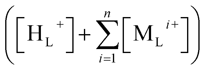“after cation exchange with TELPs as shown in the following equation with a voltage unit (V in volts)”:

where C/S represents the “specific membrane capacitance per unit surface area”, l represents the “thickness of TELP layer”, F is the “Faraday constant”, [H_L⁺] represents the “TELP concentration”, and represents the “sum of transmembrane-electrostatically localized cations (e.g., Na⁺ and K⁺) concentrations [M_Lⁱ⁺] at the liquid–membrane interface on the extracellular membrane surface after the proton–cation exchange reaching equilibrium”. Note, the is the TELC concentration.

Based on the transmembrane potential equation (eqn (1)), the “TELCs surface population density” can be readily calculated as the amount (TELC number) of “transmembrane-electrostatically localized protons/cations charges per extracellular membrane surface area (S)” using the following formula:

where N_A is the Avogadro constant (6.02205 × 10²³ mol⁻¹).

More research efforts are needed to better understand protonic bioenergetics such as to the question of what is the protonic transmembrane attraction force that holds the TELPs-membrane-TELAs capacitor together? In this article, we will calculate the protonic transmembrane attraction force through a new formulation (eqn (3)) and better elucidate some wonderful experimental observations with a transient “protonic front” in a water droplet. The analyses results will be discussed in relation to some quite interesting arguments^37,38 recently appeared in the literature.

2. TELC held by transmembrane electrostatic attraction force

Accordingly, TELPs and TELAs are held together across a fully dehydrated alkane core membrane (2.5–3.5 nm thick) by their mutual transmembrane-electrostatic attractive force as shown in a TELPs-membrane-TELAs capacitor (Fig. 1). As a result, TELPs are likely located primarily within the first layer of molecules (in the 0.3 nm thick intermediate region) on the alkane core membrane surface, whereas TELAs are located similarly in the first layer of molecules at the other side of the alkane core membrane. Therefore, the electrostatic interaction between a TELP and a TELA is across the alkane core membrane which has a known dielectric constant of about 1.88. Other factors like “ion screening, dielectric heterogeneity, or water dynamics” have little relevance here in the alkane core membrane. On the other hand, the electrostatic repulsion force among the “same side” ions such as that among TELPs (or among TELAs) is parallel to the membrane surface and orthogonal to the transmembrane attractive force vector, so that it does not affect the transmembrane attractive force but may help to spread themselves along the liquid–membrane interface.

In a protonic membrane capacitor (Fig. 1), the transmembrane attractive force is likely to be stronger than that of a single-charge-pair calculation since a transmembrane-electrostatically localized proton (H⁺) may interact with multiple transmembrane-electrostatically localized hydroxide (OH⁻) anions across the membrane as illustrated in Fig. 2.

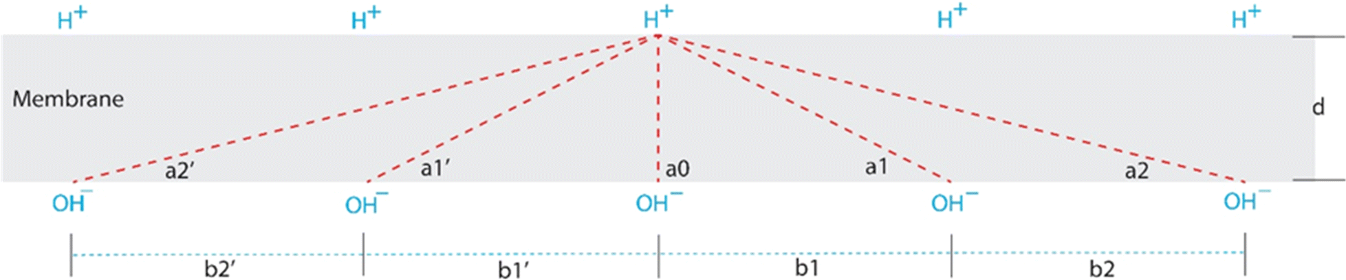Fig. 2 Illustration of a membrane cross section showing how a transmembrane-electrostatically localized proton (H⁺) (TELP) at the positive (p) side is attracted across the membrane by many transmembrane-electrostatically localized hydroxides anions (OH⁻) (TELAs) at the negative (n) side. d is a membrane thickness; b_i (such as b1 and b2) is a distance between any two adjacent OH⁻ anions with a mean separation distance of b; and a_i (such as a1 and a2) is an angle between a membrane–liquid interface line and an electrostatic interaction line between a transmembrane-electrostatically localized proton (H⁺) (TELP) and a transmembrane-electrostatically localized hydroxide (OH⁻) (TELA).

The total transmembrane attractive force (F) of a transmembrane-electrostatically localized proton (H⁺) (TELP) interacting with its multiple transmembrane-electrostatically localized hydroxide (OH⁻) anions (TELAs) can be calculated through the following equation.

where q is a protonic charge of 1.60 × 10⁻¹⁹ C and q' is a hydroxide charge of −1.60 × 10⁻¹⁹ C; κ is a dielectric constant of a membrane and ε₀ is the permittivity constant; d is a membrane thickness; b is a mean space separation distance between two adjacent hydroxides (anions) in a transmembrane-electrostatically localized anions (OH⁻) molecular layer along the liquid–membrane interface; γ is a dimensional factor: γ = 2 for a single 2-dimensional cross section system (as illustrated in Fig. 2); and γ may be about 8 (or larger than 8 if membrane thickness d is larger than that of a typical biological membrane) for a 3-dimensional membrane protonic capacitor; a_i is an angle between a membrane–liquid interface line and an electrostatic interaction line between a transmembrane-electrostatically localized proton (H⁺) and transmembrane-electrostatically localized hydroxide (OH⁻); n(+1) are the numbers of transmembrane-electrostatically localized hydroxide (OH⁻) anions that a transmembrane-electrostatically localized proton (H⁺) can electrostatically interact with; and i is the number of electrostatic interaction lines between a transmembrane-electrostatically localized proton (H⁺) and transmembrane-electrostatically localized hydroxide (OH⁻) in addition to the primary charge pair interaction (vertical line) expressed in the first term of eqn (3).

Note, the value of sin(a_i) can be calculated from the following relation.

Using specific membrane capacitance C/S of 9.2 mF m⁻² based on measured experimental data³⁹ through eqn (1) and (2) for transmembrane potential in a range from 10 to 200 mV, we calculated the associated TELC (TELP or TELA) surface density to be in a range from 562 to 11 200 charges per μm² (Table 1). The inverse of TELC surface density (1/[TELC surface density]) represents a mean membrane surface area per TELC, which was calculated to be in a range from 1780 to 89 nm² per TELC (TELP or TELA). By taking the square root of the mean surface area per TELC charge, we have, now for the first time, calculated the mean separation distance (b) between adjacent transmembrane-electrostatically localized hydroxide (OH⁻) anions (TELAs) to be in a range from 42.2 to 9.43 nm (Table 1).

Table 1 Transmembrane-electrostatically localized charges (TELPs (TELCs) or TELAs) surface density, mean separation distance (b) between adjacent transmembrane-electrostatically localized hydroxide (OH⁻) anions, and the integrated protonic transmembrane attractive force (F) calculated as a function of transmembrane potential Δψ using eqn (3) and (4) with γ = 8 and i employed in a range from 1 to n of at least 12 (and larger) for a typical lipid bilayer assuming its hydrocarbon core membrane dielectric constant (κ) of 1.88 (using dielectric constant 1.88 of hexane for hydrocarbon). TELCs density was calculated from transmembrane potential in a range from 10 to 200 mV through eqn (1) and (2) using specific membrane capacitance C/S of 9.2 mF m⁻² based on measured experimental data.³⁹ Mean separation distance b (nm) between adjacent transmembrane-electrostatically localized hydroxide (OH⁻) anions was calculated from the square root of 1/TELC density

Transmembrane potential Δψ (mV)	Transmembrane-electrostatically localized charges per μm^2	Membrane area (nm^2) per TELC	Separation distance b (nm)	Across 2.5 nm thick membrane: transmembrane attractive force (newton)	Across 3.5 nm thick membrane: transmembrane attractive force (newton)
10	5.62 × 10^2	1780	42.2	1.96 × 10^−11	1.01 × 10^−11
20	1.12 × 10^3	890	29.8	1.97 × 10^−11	1.02 × 10^−11
30	1.69 × 10^3	593	24.4	1.98 × 10^−11	1.03 × 10^−11
40	2.25 × 10^3	445	21.1	1.99 × 10^−11	1.04 × 10^−11
50	2.81 × 10^3	356	18.9	2.00 × 10^−11	1.06 × 10^−11
55	3.09 × 10^3	324	18.0	2.01 × 10^−11	1.07 × 10^−11
60	3.37 × 10^3	297	17.2	2.02 × 10^−11	1.08 × 10^−11
70	3.93 × 10^3	254	15.9	2.03 × 10^−11	1.10 × 10^−11
80	4.49 × 10^3	223	14.9	2.05 × 10^−11	1.12 × 10^−11
90	5.06 × 10^3	198	14.1	2.06 × 10^−11	1.14 × 10^−11
100	5.62 × 10^3	178	13.3	2.08 × 10^−11	1.16 × 10^−11
110	6.18 × 10^3	162	12.7	2.10 × 10^−11	1.18 × 10^−11
120	6.74 × 10^3	148	12.2	2.11 × 10^−11	1.21 × 10^−11
130	7.30 × 10^3	137	11.7	2.13 × 10^−11	1.23 × 10^−11
140	7.86 × 10^3	127	11.3	2.15 × 10^−11	1.25 × 10^−11
150	8.43 × 10^3	119	10.9	2.17 × 10^−11	1.28 × 10^−11
160	8.99 × 10^3	111	10.5	2.19 × 10^−11	1.31 × 10^−11
170	9.55 × 10^3	105	10.2	2.21 × 10^−11	1.33 × 10^−11
180	1.01 × 10^4	98.9	9.94	2.24 × 10^−11	1.36 × 10^−11
190	1.07 × 10^4	93.7	9.68	2.26 × 10^−11	1.39 × 10^−11
200	1.12 × 10^4	89.0	9.43	2.28 × 10^−11	1.41 × 10^−11

---

The data of the mean membrane surface area per TELC and the separation distance (b) between adjacent TELCs as a function of transmembrane potential as listed in Table 1 could be highly valuable to researchers in the fields of cellular and molecular energetics. As shown in Table 1, at a moderate transmembrane potential of 100 mV, the mean membrane surface area per TELC is 178 nm² per TELC (excess charge), which translates to a separation distance (b) of 13.3 nm between adjacent TELCs. With this new knowledge, readers now can judge whether certain computer simulations that were conducted far out of the range from 1780 to 89 nm² per TELC could be applicable to biological systems or not. For example, the interesting computer simulations recently published by Mallick and Agmon⁴⁰ employed a quite small membrane system that consisted of only “8 lipids in each leaflet, along with 458 water molecules, resulting in a total of 3518 atoms. The system was placed in a rectangular box with edge lengths of 22.4 × 22.4 × 65.2 Å”. They put as many as 3 excess protons into such a small system (2.24 × 2.24 × 6.52 nm) that far exceeds the expected TELC density range from 5.62 × 10² to 1.12 × 10⁴ excess charges per μm² of membrane surface area (Table 1). According to the mean membrane surface area of 178 nm² per TELC, to properly simulate the collective activity of 3 excess protons, it may require a much larger membrane system (ideally 3 × 178 nm²) that may require much larger computational powers.

Furthermore, from the data listed in Table 1, it is now revealed, for the first time, that the transmembrane potential may affect the transmembrane attractive force (F) of a transmembrane-electrostatically localized proton (H⁺) interacting with multiple transmembrane-electrostatically localized hydroxide (OH⁻) anions by its effect on influencing the mean separation distance (b). Using the mean separation distance (b) between adjacent transmembrane-electrostatically localized hydroxide (OH⁻) anions, the hydrocarbon core membrane thickness d (2.5 or 3.5 nm) and dielectric constant κ (using dielectric constant 1.88 of hexane for hydrocarbon membrane), we then calculated the transmembrane attractive force (F) of a transmembrane-electrostatically localized proton (H⁺) interacting with multiple transmembrane-electrostatically localized hydroxide (OH⁻) anions through eqn (3) and (4).

As listed in Table 1, with a transmembrane potential Δψ (mV) in a range from 10 to 200 mV, the protonic transmembrane attractive force (F) was calculated to be in a range from 1.96 × 10⁻¹¹ to 2.28 × 10⁻¹¹ newton (N) across a 2.5 nm thick membrane and in a range from 1.01 × 10⁻¹¹ to 1.41 × 10⁻¹¹ N across a 3.5 nm thick membrane. As shown in Fig. 3, the relationship between transmembrane potential Δψ (mV) and the protonic transmembrane attractive force (F) is nonlinear.

Fig. 3 Protonic transmembrane-electrostatic attractive force (N) as a function of transmembrane potential in a range from 10 to 200 mV.

The calculation results (Table 1 and Fig. 3) show: the higher the transmembrane potential the larger the transmembrane attractive force. At a high transmembrane potential such as 200 mV, since its associated mean separation distance b is smaller (9.43 nm) than that (42.2 nm) of 10 mV, the protonic transmembrane attractive force can be as large as 2.28 × 10⁻¹¹ newton (N) across a 2.5 nm thick hydrocarbon core membrane. On the other hand, at a low transmembrane potential region such as 10 mV, the associated mean separation distance b is larger (42.2 nm) so that the protonic transmembrane attractive force could approach to that (the first term in eqn (3)) for a single pair of excess proton (positive charge) and excess hydroxide (negative charge) alone across a 2.5 nm thick alkane core membrane (using dielectric constant 1.88 of hexane^41,42 for alkane), which was calculated to be 1.96 × 10⁻¹¹ N.

That is, the protonic transmembrane attractive force across a 2.5 nm thick membrane increases only slightly (by 16%), from 1.96 × 10⁻¹¹ N at 10 mV to 2.28 × 10⁻¹¹ N at 200 mV, despite a 20-fold increase in transmembrane potential. The nonlinear relationship between transmembrane potential and protonic transmembrane attractive force is due to the following two aspects: (1) the nonlinearity between the transmembrane potential and the mean separation distance b (Table 1); and (2) the nonlinearity between the separation distance b and transmembrane attractive force (eqn (3) and (4)). The nonlinear relationship due to these two aspects explains why such a substantial change (20-fold increase) in transmembrane potential results in only a minimal (16%) increase from 1.96 × 10⁻¹¹ N to 2.28 × 10⁻¹¹ N in transmembrane attractive force as shown in Fig. 3.

At a moderate transmembrane potential such as 100 mV, the integrated protonic transmembrane attractive force calculated through eqn (3) and (4) (with γ = 8 and i used in a range from 1 up to n of 12) is 2.08 × 10⁻¹¹ N across a 2.5 nm thick membrane and 1.16 × 10⁻¹¹ N across a 3.5 nm thick membrane. Accordingly, to move such a localized proton away from the membrane–liquid interface by 1 nm (say from 2.08 × 10⁻¹¹ N of 2.5 nm to 1.16 × 10⁻¹¹ N of 3.5 nm), it would require 1.62 × 10⁻²⁰ J of energy (=10⁻⁹ m × (2.08 × 10⁻¹¹ + 1.16 × 10⁻¹¹ N)/2), which is equivalent to 3.8 times as much as the Boltzmann kT thermal kinetic energy at a physiological temperature of 37 °C (310 K). These results (Table 1) again indicate that a TELPs-membrane-TELAs capacitor (Fig. 1 and 2) can be quite stable.

Notably, the hydroxide–hydroxide (OH⁻–OH⁻; TELA–TELA) repulsion force (Fig. 2) along membrane surface is orthogonal to the transmembrane attractive force vector. Therefore, the TELA–TELA (hydroxide–hydroxide) repulsion force will help to keep themselves spreading apart on membrane surface, but it will not affect the transmembrane attractive force vector. Similarly, the proton–proton (H⁺–H⁺; TELP–TELP) repulsion force along membrane surface (Fig. 2) is also orthogonal to the transmembrane attractive force vector; it will not affect the transmembrane attractive force vector but can help to keep TELPs spreading apart on membrane surface.

The charges of hydrated lipid head groups (Fig. 1) are already shielded and equilibrated with the surrounding water molecules and ions as part of the “electric double layer” associated with the “surface membrane potential” that is consistent with the Gouy-Chapman and Stern theories,⁴³ before biological energization of the membrane with formation of TELP capacitor-associated transmembrane potential. Furthermore, the lipid head groups-associated electrostatic force vectors (if any) at the two sides of the membrane are typically symmetric so that they commonly have no net effect on TELPs. In addition, there are plenty of water molecules in between the lipid head groups for excess protons to conduct through water molecules with the “hop and turn” mechanism to reach the hydrophobic alkane core membrane surface to form TELP(s) (Fig. 1 and 2).

As previously reported,^1–3 non-proton cations such as Na⁺ and K⁺ could in some extent also occupy the TELP layer through the process of cation–proton exchange. Therefore, the TELP theory is now also known as the TELC model.³³ The cation–proton exchange does not change the transmembrane potential and thus the TELP (TELC) transmembrane attractive force also remains unchanged.

3. TELP(s) formation without requiring any potential well/barrier in liquid phases

As analyzed above, since transmembrane-electrostatically localized protons (TELPs) are held by the attractive force (Table 1 and Fig. 3) with the transmembrane-electrostatically localized hydroxides anions (TELAs) across the membrane (Fig. 1 and 2), TELP does not necessarily “bind” to the surface; nor does the TELP(s) formation require any potential barrier in any of the liquid phases. Therefore, TELPs are different from the prior population of protons that are somehow bonded or attracted by fixed charge groups (e.g., lipid head groups) and/or other fixed property at the membrane surface. Those non-TELP (lipid head group-attracted) protons are irrelevant to protonic motive force, since they are there before the membrane system is energized through the formation of TELPs. Similarly, the so called “enriched protons” that were claimed by Silverstein³⁷ to be “enriched” by the liquid–decane interface or air–water interface are also irrelevant to protonic motive force since they are not TELPs. This is true because those protons would have to be “enriched” by a type of fixed interface property such as the putative “potential well/barrier” near the “air–water interface”, as Silverstein mentioned “where the amphiphilic hydrated proton is believed to be better accommodated in terms of hydrophobic force and water–water H-bond network disruption” which (even if exist) would occur before the membrane system is energized through TELP(s) formation.

Silverstein's “Table 1” of the “critique”³⁷ lists “surface pH (pH_surf)” in a range “from 4.4 to 6.6 at the water/hydrophobic interface and the lipid bilayer surface, and from 5.5 to 7.1 at the surface of functioning bioenergetic membranes”. However, none of them has any relevance to TELPs that are transmembrane-potential-dependent. For example, many of the numbers are from molecular dynamic simulations for the fixed interface property-enriched protons (at the liquid–decane interface or air–water interface) without any transmembrane potential and its membrane capacitor-associated TELP(s), thus having little relevance to the TELP(s) model. The measured mitochondrial “pH 6.8–7.0” and “pH 7.0–7.1” that he listed in his “Table 1” are obviously the bulk-phase pH values (not really “surface pH (pH_surf)” as he seems to have claimed). Therefore, the “critique”³⁷ based on his “Table 1” again seems reflecting some misunderstanding of the TELP model. Recently, Silverstein repeated his misconceived arguments.⁴⁴ Independent researcher has now also pointed out that “Silverstein's critiques are untenable”.⁴⁵

As discussed previously,⁴ according to the size of the pH-sensitive GFP⁴⁶ and its associated protein linker used in the mitochondrial pH measuring experiments,^47–49 “the active site of its pH-sensitive chromophore is likely to be at least about 2–3 nm away from the membrane surface”. This separation distance (2–3 nm away from the mitochondrial membrane surface) is good to detect bulk-liquid phase pH; but too far away to sense TELPs on the alkane core membrane surface. Therefore, according to the TELPs model (Fig. 1), we predict that the pH-sensitive GFP sensors can see the protons in the bulk liquid phase (around pH 7), but could not detect TELPs that stay primarily within the first layer of water molecules on the hydrophobic alkane core membrane surface. This TELPs-model-based prediction for the pH-sensitive GFP bulk-liquid phase pH measurement was observed exactly in the measured mitochondrial “pH 6.8–7.0”⁴⁷ and “pH 7.0–7.1”⁴⁹ that Silverstein listed in his “Table 1”.³⁷ Therefore, readers can now see that the data listed on Silverstein's “Table 1” are in line with the TELPs-model prediction.

According to our understanding with the TELC(s) model,^1–3 TELCs (TELPs) activities “are likely to be dynamic”. “Although they are in dynamic communication with the bulk aqueous liquid phase through the cation–proton exchange process, most of the TELPs are likely to stay within the first layer of water molecules on the hydrophobic core membrane surface which is beneath the membrane's lipid head groups” (Fig. 1). That is, TELPs likely are just hiding on the alkane core membrane surface beneath the lipid head groups. Currently, we are not aware of any artificial pH sensor that could be used to directly measure TELPs in biomembrane systems, that probably could explain why the existence of TELPs was never uncovered during the last seven decades of the “delocalized vs. localized proton coupling debates” since the early 1960s.^50–59 Only recently, TELPs were, for the first time, discovered through experimental demonstration of a protonic capacitor in a biomimetic cathode water-membrane-water anode system using an Al metal film as a protonic sensor.⁹ However, the Al film-based protonic sensor would be not easy for use in micro/nanometer-scale biomembrane systems. Therefore, it is now important to develop “a new type of protonic sensors to directly observe TELPs within the first layer of water molecules on hydrophobic core membrane surface in biological membrane systems”. According to our analysis, two natural membrane protein complexes are now known to sense and use TELPs: the F_oF₁-ATP synthase⁴ and the melibiose transporter MelB.³¹ Therefore, I hereby encourage researchers “to take cue and inspiration from the natural TELPs-sensing biomolecules to better design and make the needed protonic probes for more direct detections of TELPs in biomembrane system.”

4. The Zhang et al. 2012 experiment could be explained by a transient “protonic front” in a water droplet

The “critique”³⁷ claims that the putative “potential well/barrier model” of Junge and Mulkidjanian^59,60 was “supported by Pohl's group⁶¹”. In his previous publication,⁶² Silverstein even grossly claimed it “seems to rule out Lee's model”. In contrast, as we recently reported,⁶³ the experimental results of Pohl's group⁶¹ can actually be well explained by the protonic conduction fundamentals (liquid water as a protonic conductor) of the TELPs model, but not really by the putative “potential well/barrier model”.

As shown in Fig. 4, Pohl's group⁶¹ elegantly “performed a wonderful experiment by injecting approximately 1 fl of hydrochloric acid (HCl) into an aqueous liquid droplet (140 μl) under decane oil and then monitor the appearance of protons (H⁺) at the liquid–oil interface with a proton-sensitive fluorescent dye Oregon Green 488 1,2-dihexadecanoyl-sn-glycero-3-phosphoethanolamine”. Their experimental results⁶¹ can now be better elucidated by the fundamental understanding of liquid-water “protonic conduction” that is associated with the TELPs theory, but not TELPs per se; The Zhang et al. 2012 (Pohl's group⁶¹) experiment likely involved a transient “protonic front” effect in a single water droplet system which has no transmembrane potential and no TELPs.

Fig. 4 The water droplet experiment with a transient protonic front: “experimental scheme for fluorometrical detection of lateral proton diffusion that can now be explained with the protonic conduction fundamentals of the TELP model: protons (red H⁺) can spread far ahead of the slow diffusing chloride anions (red Cl⁻), resulting in a transient effect of excess protons. On top of a water droplet (140 μl) containing 0.1 or 1 mM Mes, the experimental team (Zhang et al. 2012)⁶¹ added n-decane (280 μl) containing 0.7 μM of fluorescent dye Oregon Green 488 1,2-dihexadecanoyl-sn-glycero-3-phosphoethanolamine, which accumulated at the interface. The protons were injected at a distance < 1 μm from the interface through a glass pipette with a tip diameter of ≈1 μm filled with 0.7% HCl. The injection volume was small (approximately 1 fl) so that convection had negligible effect on diffusion. The dye was excited at 485 nm via an objective (20×) and its fluorescence was collected via the same objective after a long pass filter (515 nm). The fluorescent microscope (Olympus IX70, Tokyo, Japan) was equipped with two sets of diaphragms (TILL Photonics, Munich, Germany), which allowed the selection of the emission (5 × 5 μm) and excitation (10 × 10 μm) areas”. Adapted and modified from ref. 61 with copyrights permission.

According to the knowledge of protonic conduction as one of the fundamentals in the TELC model (1, 2), “liquid water can serve as a protonic conductor based on the ‘hops and turns’ mechanism as first outlined by Grotthuss”.^64–67 Therefore, as we recently reported,⁶³ the “spread of protons from the hydrochloric acid (HCl) in the liquid” is expected to be “much faster than that of the chloride anions (Cl⁻) which could slowly spread only through diffusion”. Because the protons can quickly spread as a “protonic front” far “ahead of the slow diffusing chloride anions (Cl⁻)”, it temporally creates “a transient effect of excess protons because of their mutual electrostatic repulsion to temporally spread from the bulk liquid phase towards the liquid–oil interface where they may be detected by proton-sensitive fluorescent dye Oregon Green 488” as illustrated in Fig. 4. “When the chloride anions (Cl⁻) finally catch up with the protons (H⁺) so that all the protonic charges will be balanced with the chloride anions (Cl⁻) again as that in a typical equilibrated HCl solution, the effect of the transient excess protons will end so that the protons that have reached the liquid–oil interface will all move out of the liquid–oil interface and return to the bulk liquid phase”. This explains the effect of transient “excess protons” from “its beginning to its end typically in a few seconds after the injection of HCl solution”. Remarkably, this effect of transient “excess protons” as illustrated in Fig. 4 with our understanding of liquid water as a protonic conductor is “well in line with the result of an independent study⁶⁸” which also rightly pointed out that “the excess protons propagate as an advancing front”.

The effect of the transient “excess protons” that tends to make themselves spreading to the liquid–oil interface at the edge of a liquid droplet can be explained by the well-known electrostatic effect of a conductor (Fig. 5) where any extra charges will repel each other and distribute themselves to the edge of the conductor. One can mathematically justify this property “by using the Gauss law equation of electrostatics and the fact that there can be no electric field E inside a conductor. Gauss's law relates the net charge Q within a volume to the flux of electric field lines through the closed surface surrounding the volume” as expressed in the following Gauss law equation,⁶⁹

where ε₀ represents “the electric permittivity constant” and dS represents “a differential surface element”. Here the “small circle on the integral sign” shows that “the integration is performed over the closed surface”. Consider then “a series of applications, where a small volume at the center of the conductor is gradually increased until it is just inside the conductor surface, indicated by r” in Fig. 5. By definition, “the electric field E is zero everywhere in a conductive body”. In each case, “since E = 0 everywhere inside the conductor (the liquid water droplet as a protonic conductor), the left side of eqn (5) vanishes and therefore the right side must also vanish, which means that no net charge (Q = 0) is within the volume”; the excess charges (the excess protons in the case of a liquid droplet) must therefore be on the conductor surface (the liquid water droplet surface: the liquid–oil interface).

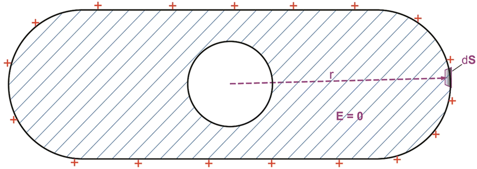Fig. 5 Closed Gaussian surface inside a volume of conducting materials showing a common physical phenomenon: in a conductor at static equilibrium, all the (extra) electric charge resides on the surface of the conductor.⁶⁹

As mentioned above, this transient “excess protons” electrostatic effect in a liquid droplet of Zhang et al. 2012 experiment is expected to be short lived for a few seconds; since the effect of the transient “excess protons” will end “when the chloride anions (Cl⁻) finally catch up” with the protonic (H⁺) front (Fig. 4) “so that all the protonic charges will then be balanced with the chloride anions (Cl⁻) again as that in a typical equilibrated HCl solution”.

Note, the root mean square distance (x̄) traveled by diffusing particle is and its value can be calculated using the following textbook equation.⁷⁰

Here, D is a diffusion coefficient, m is the dimension of the particle's Brownian motion, and t is the time. When m = 1, the probability distribution of the magnitude of the particle's mean squared displacement (2Dt) from its original position in 1-dimension diffusion is Gaussian.

Use of eqn (6) can calculate the diffusion time (t) required to travel for a given distance x̄ as well. Table 2 lists our calculated results using the known diffusion coefficient D of 9.31 × 10⁻⁹ m² s⁻¹ and 2.03 × 10⁻⁹ m² s⁻¹, respectively, for H⁺ and Cl⁻ in liquid water.⁷¹ As shown in Table 2, the 1-dimensional (m = 1) diffusion time (t) for protons (H⁺) to travel the root mean square distance x̄ of 45 μm was calculated to 0.11 s, which is shorter than that (0.50 s) for Cl⁻ to travel the same distance of 45 μm. That is, about 0.11 s after the injection of HCl solution, the root mean square distance x̄ traveled by protons (H⁺) was calculated to be 45 μm, which as a “protonic front” appears rightly within the experimental monitoring range from 35 to 85 μm in Pohl's group experiment.⁶¹ On the other hand, the distance x̄ traveled by chlorides (Cl⁻) with the same amount of time (0.11 s) was calculated to be only 21 μm that is still not in the detection range of 35–85 μm. These calculated results support the understanding that the “protonic front” can be transiently well ahead of the slow-diffusing chlorides (Cl⁻) as illustrated in Fig. 4.

Table 2 Comparison of the experimentally observed transient H⁺ peak–quenched fluorescence signal valley-bottom (at the maximal fluorescence depletion time, τ_max) with the 1-dimensional (m = 1) and 2-dimensional (m = 2) diffusion time (t) required to travel the root mean square distance x̄ of 45, 65, and 85 μm that were calculated with eqn (6) using the known diffusion coefficient D of 9.31 × 10⁻⁹ m² s⁻¹ and 2.03 × 10⁻⁹ m² s⁻¹, respectively, for H⁺ and Cl⁻ in liquid water.⁷¹ Transient H⁺ peak time (τ_max) was obtained from the experimental data curves of Fig. 6⁶¹ through analysis using the WebPlotDigitizer which is a computer vision assisted software that helps extract numerical data from images of a variety of data visualizations⁷²

Diffusing ions	H^+	Cl^−
Diffusion coefficient D	9.31 × 10^−9 m^2 s^−1	2.03 × 10^−9 m^2 s^−1
1-D diffusion time (t) required to travel 45 μm	0.11 s	0.50 s
2-D diffusion time (t) required to travel 45 μm	0.05 s	0.25 s
Transient H^+ peak time (τmax) measured at 45 μm	0.10 s
1-D diffusion time (t) required to travel 65 μm	0.23 s	1.04 s
2-D diffusion time (t) required to travel 65 μm	0.11 s	0.52 s
Transient H^+ peak time (τmax) measured at 65 μm	0.16 s
1-D diffusion time (t) required to travel 85 μm	0.39 s	1.78 s
2-D diffusion time (t) required to travel 85 μm	0.19 s	0.89 s
Transient H^+ peak time (τmax) measured at 85 μm	0.31 s

---

As listed in Table 2, the 1-dimensional diffusion time (t) required for H⁺ to travel 65 μm and 85 μm from the point of hydrochloric acid (HCl) injection was calculated respectively to be 0.23 and 0.39 s, which are shorter than those (1.04 and 1.78 s) for Cl⁻ to travel the same distance of 65 and 85 μm. The diffusion time (t) required for Cl⁻ to travel 85 μm was calculated to be 1.78 s while it would take only 0.39 s for H⁺ to travel the same 85 μm. These results again indicate a transient Gaussian “protonic front” followed by a relatively slow diffusing/lagging Gaussian “chloride front” during the process.

Since the liquid droplet in the experiment (Fig. 4) had a finite height and was not entirely flat, there could be an effect of 2-dimensional diffusion from the point of hydrochloric acid (HCl) injection to the proton-sensing fluorescent molecular probes (fluorescent dye Oregon Green 488 1,2-dihexadecanoyl-sn-glycero-3-phosphoethanolamine) located along the water–decane interface. Therefore, we have now calculated the 2-dimensional diffusion time required to travel to the detection sites. As listed in Table 2, the 2-dimensional diffusion time required for protons (H⁺) to travel to the 45, 65, and 85 μm detection sites is now calculated respectively to be 0.05, 0.11, and 0.19 s. Whereas, the 2-dimensional diffusion time required for by chlorides (Cl⁻) to travel to the same 45, 65, and 85 μm detection sites is calculated to be 0.25, 0.52 and 0.89 s, respectively.

We predict that the experimentally measured transient H⁺ peak time (τ_max) must land within the domain somewhere between the 1-D diffusion time (t) and 2-D diffusion time (t). As shown in Table 2, this predicted feature was exactly observed in the Pohl's group⁶¹ experiment. For example, the transient H⁺ peak time (τ_max) of 0.10 s observed at detection site of 45 μm appeared indeed in the domain between the calculated 1-D diffusion time (t) of 0.11 s and the 2-D diffusion time (t) of 0.05 s. Similarly, the transient H⁺ peak time (τ_max) of 0.16 s measured at 65 μm was also within the domain between the calculated 1-D diffusion time (t) of 0.23 s and 2-D diffusion time (t) of 0.11 s; the transient H⁺ peak time (τ_max) of 0.31 s measured at 85 μm was within the domain between the calculated 1-D diffusion time (t) of 0.39 s and 2-D diffusion time (t) of 0.19 s as well. These results showed that the 1-dimensional diffusion-based x̄ vs. t calculation represents a quite reasonably good prediction for the observed “protonic front” phenomena; the effect of 2-dimensional diffusion (if any) is minor in this case.

Anyhow, the diffusion “time (τ_max) that it takes after the injection of the HCl solution for the appearance of the maximum peak fluorescence quenching (depletion) signal should depend on the distance (x) from the point of the HCl injection to the spot of the Oregon Green 488 fluorescence detection.⁶¹ The whole transient event from its beginning to its end should be just for a few seconds that the system takes for its equilibration. These predicted features were observed exactly in the experiment”, where a linear dependence of x² on τ_max was found.⁶¹

From here, we now understand that the protonic fluorescence signal from the dye Oregon Green 488 at the liquid–oil interface in the Pohl's group⁶¹ experiment may reflect the transient “protonic front” effect. For instance, when the transient “protonic front” entering the detection site at the distance of x = 45 μm (blue dots curve in Fig. 6) from the area of proton release, it was measured as the protonic fluorescence quenching (fluorescence intensity decrease) from the experimental time of 0.01 s until the transient H⁺ peak time (τ_max) of 0.10 s (Fig. 6) where apparently the peak transient “protonic front” (which may be represented by the 1-dimensional diffusion-based x̄) fully moving into the detection site. After that, as the peak transient “protonic front” moving out of the detection site of 45 μm and the Gaussian tip of the relatively slow diffusing Cl⁻ anions (which could drive the transient excess protons out of the liquid–decane interface by charge re-neutralization) starting to enter the same detection site of 45 μm, the proton-sensitive fluorescence intensity will start to recover (increase) as shown in Fig. 6.

Fig. 6 Experimental observations: “kinetics of proton diffusion over different distances x. Each trace is the average of at least 20 records. The midpoint of the detection area was located at distances x = 45 (blue), 65 (red), and 85 (green) μm from the area of proton release. The H₂O buffer contained 0.1 mM Mes and 100 mM NaCl, pH 6.3. A linear dependence of x² on τ_max was found (inset)”. Reproduced from ref. 61 with copyrights permission.

We predict that when the peak transient “chloride front” (which may be represented by its 1-dimensional diffusion x̄) enters the detection site of 45 μm at the expected diffusion time of about 0.50 s, the majority (over 60%) of transient excess protons should be out of the liquid–decane interface and return to the bulk liquid phase becoming charge-balanced protons as in a typical HCl solution. This predicted feature was indeed observed also in the experimental results. As shown in Table 3, the transient H⁺ fluorescence quenching signal at the diffusion time of 0.50 s was reduced to 37% from its maximally quenched fluorescence signal level at the valley bottom (100%). Interestingly, this fluorescence curve behavior seems to represent a type of exponential decay by a factor of the mathematical constant e (1/e = 0.37). Similarly, the transient H⁺ fluorescence quenching curves that were measured at the sites of 65 and 85 μm decayed to 24% and 22% of their respective peak values when the peak transient “chloride front” enters the same detection sites (of 65 and 85 μm) at the diffusion time of 1.04 and 1.78 s (Table 3). In all the cases, the transient H⁺ fluorescence quenching signal finally decayed toward zero in a few seconds that the system takes for its equilibration (Fig. 6). This explains the phenomenon of the transient “protonic front” from its beginning to the end.

Table 3 Calculation of percentage H⁺ population at the diffusion time (t) that is required for chloride to ravel its root mean square distance x̄ of 45, 65 and 85 μm. The transient H⁺ peak time (τ_max), transient H⁺ peak-quenched fluorescence signal value, and H⁺ quenched fluorescence signal at each of the chloride x̄ diffusion time points of 0.50, 1.04, and 1.78 were obtained from the experimental data curves of Fig. 6⁶¹ through analysis using the WebPlotDigitizer which is a computer vision assisted software that helps extract numerical data from images of a variety of data visualizations.⁷² The % H⁺ population at each of the chloride x̄ time points was calculated from the ratio of H⁺-quenched fluorescence signal at chloride x̄-based diffusion time points to the transient (τ_max) H⁺ peak-quenched fluorescence signal (valley bottom level)

Distance from the HCl injection site to the detection site	H^+ peak-quenched fluorescence (valley) time (τmax)	Transient (τmax) H^+ peak-quenched fluorescence signal valley level	Diffusion time of chloride x̄	H^+ quenched fluorescence signal at diffusion time of chloride x̄	% H^+ population at the diffusion time of chloride x̄
45 μm	0.10 s	−11.36	0.50 s	−4.23	37%
65 μm	0.16 s	−8.96	1.04 s	−2.18	24%
85 μm	0.31 s	−5.90	1.78 s	−1.28	22%

---

Notably, the “protonic front” likely has a diffusing Gaussian distribution, which has an extended Gaussian spearhead before the central Gaussian peak at the position of the root mean square distance (x̄) and followed by its extended Gaussian tail. Therefore, as the Gaussian “protonic front” with its extended Gaussian spearhead first enters the detection site (for example at 45 μm), then the fluorescence intensity decreases when protons reach the fluorescent reporter at the liquid–oil interface. When the Gaussian “protonic front” central peak (at the root mean square distance (x̄)) reaches the measuring point, it will result in maximal fluorescence depletion (τ_max = 0.10 s) as experimentally demonstrated (Fig. 6). After that, as the Gaussian “protonic front” peak and its extended Gaussian tail leaving the measuring point and/or the Gaussian spearhead of the slow diffusing “chloride front” gradually enters the detection site, it will result in a gradual increase in fluorescence intensity when protons leave the detection area. When the Gaussian “chloride front” peak enters the detection area, majority (over 60%) of the transient excess protons will be out of the liquid–decane interface. When the system finally reaches its equilibrium in a few seconds, all the transient excess protons will be out of the liquid–oil interface and become charge-balanced bulk-liquid protons as in a typical HCl solution; Consequently, the fluorescence signal will continue rising and finally approaching the original level of zero.

Since “the protonic conduction from the point of the HCl injection to the spot of the Oregon Green 488 fluorescence detection is likely through the bulk liquid phase”, we predict that “the use of increasing buffer capacity such as from 0.1 mM Mes to 1 mM Mes will slow down the protonic conduction” (since the buffer could take up some of the injected acid and the diffusion of the buffer Mes is slow) and thus “slow the appearance of the fluorescence signal with reduced amplitude”. Furthermore, when replacing H₂O by D₂O, we predict that “the appearance of the fluorescence signal will be slower with somewhat reduced amplitude, since D⁺ is heavier than H⁺, which will thus slow the “hops and turns” conduction mechanism”. All these predicted features were also confirmed through the experimental observation.⁶¹

As recently reported,⁶³ we further predicted that “the use of NaCl solution would somewhat enhance the effect of the transient excess protons since the higher NaCl concentration could slightly impede the spread of the Cl⁻ from the injected HCl solution relatively to the H⁺ conduction. Thus, the amount of time that takes from the HCl injection to the appearance of excess protons at the liquid–oil interface would get shorter (faster). This predicted feature was also exactly observed in the experiment of Fig. S1 of ref. 61”.

Therefore, as we recently discussed,⁶³ the experimental observation of Pohl's group⁶¹ seems well in line with the fundamental understanding of “liquid water as a protonic conductor”. It is important to point out that the work of Pohl's group⁶¹ does not really support the “potential well/barrier models” whose “activation barrier” height was claimed to be as high as “ΔG°^‡ ≈ 20–30 RT”.⁷³ Firstly, Silverstein's claimed “ΔG°^‡ ≈ 20–30 RT” (around + 25 RT; note, RT is the molar thermal kinetic energy expressed as the product of the gas constant R and absolute temperature T) “in the liquid water phase at the location of 0.4 nm away from the decane surface⁷³ would be equivalent to an activation barrier of about 60.9 kJ mol⁻¹; that is likely to be questionable since he has never explained how could it be possible for water molecules to form such a high activation barrier that is far much higher than their hydrogen bond energy?” An independent study⁷⁴ showed: “the water hydrogen bond Gibbs energy ΔG⁰ is 2.7 kJ mol⁻¹ (with ΔH⁰ = 7.9 kJ mol⁻¹ and TΔS⁰ = 5.2 kJ mol⁻¹)”. For the protonic mobility mechanism, “the activation energy E_A is reported to be 11.3 kJ mol⁻¹,^74,75 in contrast to Silverstein's claimed ‘ΔG°^‡ ≈ 20–30 RT’ (around 60.9 kJ mol⁻¹)”.

On the other hand, even if assuming the “potential well/barrier as proposed by Junge and Mulkidjanian^59,60 would really exist”, then “the protons from the HCl solution that was injected into the bulk liquid phase would not have been able to freely enter from the bulk liquid phase into the liquid–oil interface”. Furthermore, “if somehow the protons once get into the liquid–oil interface, then the protons would not have been able to freely get out of the liquid–oil interface to return into the bulk liquid phase if the potential well/barrier as proposed by Junge and Mulkidjanian^59,60 were really in its presence. In contrast to the potential well/barrier model, the experimental data⁶¹ demonstrated that the protons can enter from the bulk liquid phase into the liquid–oil interface” to arrive at the detection site at a distance of 45 μm from the HCl injection site in 0.10 second after the HCl injection and then completely “get out of there freely back into the bulk liquid phase” in a few seconds that the system takes for its equilibration.

Furthermore, if the “potential well” with a “negative ΔG for the depth of the potential well near the interface (4–8 RT at 1–2 Å)” as claimed in ref. 73 were true, then a transient H⁺ population that once enters the liquid–decane interface would be trapped there by the “potential well”, which (if true) would predict a steady-state proton-quenched fluorescence signal plateau that would have remained as a flat curve at the H⁺ peak-quenched fluorescence signal valley bottom level (such as −11.36) upon and after the diffusion time of 0.10 s as measured at the detection site of 45 μm or a plateau that would have appeared as a flat curve at least at a level substantially below the zero after reaching the peak proton-quenched fluorescence signal bottom level (−11.36) after the diffusion time of 0.10 s. In contrast to the “potential well” proton trap prediction, no such a proton-quenched fluorescence plateau flat curve was observed in the experimental results (Fig. 6). The observed H⁺ population-quenched fluorescence curve (Fig. 6) showed that after the fluorescence intensity decreased to the valley bottom point (−11.36 at the diffusion time of 0.10 s as measured at the detection site of 45 μm), the fluorescence signal rises from the valley bottom point (−11.36; 0.10 s) all the way up to the zero level when the system reaches its equilibrium within a few seconds. That is, the experimentally observed H⁺ sensitive fluorescence curve (Fig. 6) itself rejected the “potential well/barrier models”. All these indicate that either the putative potential well/barrier as proposed by Junge and Mulkidjanian^59,60 and recently advocated by Silverstein⁷³ “does not really exist, or the putative potential well/barrier (even if exist) is irrelevant to explaining the experimental results of Pohl's group”.⁶¹

Therefore, as we recently reported,⁶³ the experimental results of Pohl's group⁶¹ can be explained by a transient “protonic front” effect that is consistent with our understanding of liquid water as a protonic conductor as shown in the “TELPs model,^1,2 which does not assume, nor does require, any putative potential well/barrier in the liquid phase”.

5. Improper application of the Bjerrum length by Knyazev et al. 2023

Interestingly, Silverstein and Pohl's group recently published an article³⁸ in arguing against our understanding of the transient “protonic front” effect. Unfortunately, their argument seems stemming from their improper use of the “Bjerrum length” that they considered only for a single charge pair interaction, but not for multiple charges systems like a protonic capacitor where a transmembrane-electrostatically localized H⁺ charge may be attracted by multiple transmembrane-electrostatically localized HO⁻ anions (Fig. 2). The Bjerrum length (which is named after “Danish chemist Niels Bjerrum 1879–1958”⁷⁶) is “the separation distance at which the electrostatic interaction between two elementary charges is comparable in magnitude to the thermal energy scale, k_BT, where k_B is the Boltzmann constant and T is the absolute temperature in kelvins”. Readers will soon be able to see how the improper application of the Bjerrum length approach by Silverstein and Pohl's group³⁸ to a biomimetic Teflon membrane with a thickness of 75 μm in trying to calculate the TELP transmembrane attractive force could result in erroneous numbers off by orders of magnitudes. More unfortunately, Silverstein seems keeping his erroneous analysis with “Bjerrum length” and repeatedly making flawed arguments even in his latest “critiques”.⁷⁷ Therefore, it is important to clarify this issue here for the scientific community.

To properly calculate the protonic transmembrane attractive force (F), it is important to use a proper equation like eqn (3) that includes all possible multiple charge interactions especially when the membrane thickness is larger than that of a typical biomembrane.

For example, when a membrane thickness of 75 μm is used as in a biomimetic Teflon membrane protonic capacitor,⁷ “a transmembrane-electrostatically localized H⁺ charge will be able to electrostatically interact with huge numbers of transmembrane-electrostatically localized HO⁻ anions. For instance, with a bird view angle of 45° from a membrane surface, each proton will be able to electrostatically ‘see’ through the 75 μm thick Teflon membrane for the HO⁻ anions at the other side of the membrane within an area as large as 18 000 μm² (=3.14 × (75 μm)²). For a 75 μm thick biomimetic Teflon membrane with a TELC density of 5600 electronic charges per μm², the number of transmembrane-electrostatically localized HO⁻ anions that each transmembrane-electrostatically localized proton can electrostatically interact is now estimated to be about 10⁸”. Therefore, the “Bjerrum length” approach used by Silverstein and Pohl's group⁶¹ could “miss to account for the protonic transmembrane attractive force from as many as 10⁸ TELP–TELA electrostatic interactions for each of transmembrane-electrostatically localized H⁺ charges”. Readers can now see how the improper application of the Bjerrum length approach by Silverstein and Pohl's group³⁸ to the biomimetic Teflon membrane with a thickness of 75 μm “could result in immense analysis errors off by orders of magnitudes”.

That is, the numbers n(+1) of transmembrane-electrostatically localized hydroxide (OH⁻) anions that can together electrostatically attract a transmembrane-electrostatically localized proton (H⁺) can be as large as 10⁸. Consequently, the second term (multiple interactions) of the protonic transmembrane attractive force equation (eqn (3)) becomes far more important than the first term (single charge pair) in determining the amount of protonic transmembrane attractive force. Thus, when a membrane thickness of 75 μm (that is substantially thicker than a typical biomembrane) is used in a protonic capacitor, although the first term (single charge pair attraction) of eqn (3) could decrease by orders of magnitudes, the second term (multiple interactions) could increase by orders of magnitudes because as many as 10⁸ transmembrane-electrostatically localized HO⁻ anions could now interact with each transmembrane-electrostatically localized proton.

From here, readers probably can understand why the application of “Bjerrum length” by Knyazev et al.³⁸ to the case of a 75 μm thick Teflon membrane protonic capacitor is simply wrong: Knyazev et al.³⁸ just completely missed the multiple transmembrane-electrostatic attraction effect (the second term in eqn (3)) as illustrated in Fig. 2. Consequently, their “Bjerrum length”-based claims that “the separation at which the electrostatic interaction between two elementary charges is comparable in magnitude to the thermal energy is more than two orders of magnitude smaller and, as a result, the H⁺ and OH⁻ layers cannot mutually stabilize each other, rendering proton accumulation at the interface energetically unfavorable”³⁸ are just completely groundless or misconceived. So do their claims of violating “(i) the law of electroneutrality, (ii) Fick's law of diffusion, and (iii) Coulomb's law”,³⁸ which are completely out of line.

In contrast, our TELP-based analyses as outlined previously⁶³ well follow “(i) the law of electroneutrality, (ii) Fick's law of diffusion, and (iii) Coulomb's law”. For example, the predicted transient “protonic front” charges are balanced with the slow diffusing Cl⁻ charges within the liquid droplet as we illustrated in Fig. 4 in accordance with the law of electroneutrality.

Note, TELCs (TELPs) are held at the liquid–membrane interface by the transmembrane-electrostatic attractive force as illustrated in Fig. 2 and expressed mathematically in eqn (3) in accordance with the Coulomb's law. Consequently, TELPs can quickly translocate and diffuse along the liquid–membrane interface and into the proton channel of ATP synthase to drive ATP synthesis; a fraction of TELPs could also diffuse into the bulk liquid phase during a cation–proton exchange process in accordance with the Fick's law.

As recently discussed,⁶³ we must again point out that the “transient excess protons effect” in the experiment of Pohl's group⁶¹ “was relatively weak” because there are “no excess hydroxyl anions on the other side of the oil to enhance the holding of the transient excess protons at the water–oil interface, in contrast to that of TELPs in mitochondria”. This also explains “why the experiments of Pohl's group⁶¹ showed a surface pH of only ‘2–3 units below bulk pH’ while TELPs are typically at mM levels (effective local pH about 2–3)”.^1,2

Unlike a biological membrane system, the experimental system of Pohl's group⁶¹ apparently involves an unusual transient “protonic front” effect in a single water droplet with a liquid water–oil interface, but no transmembrane potential and no true excess protons. Even its transient excess protons are just in the same liquid water droplet with the countering Cl⁻ anions, which does not resemble to any cell bioenergetic system that has a transmembrane potential with TELCs capacitor comprising excess positive charges at one side of the membrane and equal number of excess anions at the other side. Thus, the experimental system of Pohl's group,⁶¹ strictly speaking, does not qualify to be considered as any reasonable biomimetic system. Consequently, although the observations in the experiment of Pohl's group⁶¹ appear to be true, it is still questionable as to whether they could have any substantial relevance to cell energetics. That type of “study” and arguments, sometimes, could even cause unnecessary confusions in the field. For example, their recent article³⁸ passionately claims “We show that (i) the law of electroneutrality, (ii) Fick's law of diffusion, and (iii) Coulomb's law prevail”, in a manner similar to the parable with one of the blind men holding an elephant's tail and passionately claiming “elephant is a rope”.

Therefore, I hereby encourage more bioenergetics research efforts in more relevant protonic cell systems that should have transmembrane potential associated with certain TELCs-membrane-TELAs capacitor comprising excess positive charges at one side and excess anions at the other side of the membrane.

Data availability

All data generated or analyzed during this study are included in this article and in the cited references.

Author contributions

Lee designed and performed research, analyzed data, and authored the paper.

Conflicts of interest

The author declares no competing financial and non-financial interests.

Acknowledgements

The protonic bioenergetics aspect of this research was supported in part by a Multidisciplinary Biomedical Research Seed Funding Grant from the Graduate School, the College of Sciences, and the Center for Bioelectrics at Old Dominion University, Norfolk, Virginia, USA. The author thanks the Editor and anonymous peer reviewers for their highly valuable and constructive review comments that made this article better.

References

1. J. W. Lee, Heliyon, 2019, 5, e01961,  DOI:10.1016/j.heliyon.2019.e01961.
2. J. W. Lee, Sci. Rep., 2020, 10, 10304,  DOI:10.1038/s41598-020-66203-6.
3. J. W. Lee, Sci. Rep., 2021, 11, 14575,  DOI:10.1038/s41598-021-93853-x.
4. J. W. Lee, Mitochondrial Commun., 2023, 1, 62–72,  DOI:10.1016/j.mitoco.2023.09.001.
5. J. W. Lee, ACS Omega, 2020, 5, 17385–17395,  DOI:10.1021/acsomega.0c01768.
6. J. W. Lee, J. Neurophysiol., 2020, 124, 1029–1044,  DOI:10.1152/jn.00281.2020.
7. H. A. Saeed and J. W. Lee, Bioenergetics, 2015, 4(127), 1–7,  DOI:10.4172/2167-7662.1000127.
8. H. Saeed and J. Lee, Water, 2018, 9, 116–140,  DOI:10.14294/2018.2.
9. J. W. Lee, Water, 2025, 14, 35–58,  DOI:10.14294/WATER.2024.4.
10. H. Saeed, PhD thesis, Old Dominion University, Norfolk, VA 23529, USA, 2016.
11. G. Kharel, PhD thesis, Old Dominion University, Norfolk, VA 23529, USA, 2024.
12. A. Guffanti and T. Krulwich, Biochem. Soc. Trans., 1984, 12, 411.
13. T. A. Krulwich, R. Gilmour, D. B. Hicks, A. A. Guffanti and M. Ito, Adv. Microb. Physiol., 1998, 40, 401–438.
14. T. A. Krulwich, J. Liu, M. Morino, M. Fujisawa, M. Ito and D. B. Hicks, Extremophiles Handbook, 2011, pp. 119–139.
15. J. W. Lee, Bioenergetics, 2015, 4(121), 1–8,  DOI:10.4172/2167-7662.1000121.
16. J. W. Lee, PCT International Patent Application Publication Number WO 2017/007762 A1, 2017, p. 56.
17. J. W. Lee, Biophys. J., 2019, 116, 317a.
18. J. W. Lee, Abstr. Pap. Am. Chem. Soc., 2018, 255, PHYS 211.
19. J. W. Lee, Biophys. J., 2017, 112, 278a–279a.
20. J. W. Lee, Energies, 2022, 15, 7020,  DOI:10.3390/en15197020.
21. J. W. Lee, J. Sci. Explor., 2022, 36, 487–495,  DOI:10.31275/20222517.
22. J. W. Lee, J. Sci. Explor., 2023, 37, 5–16,  DOI:10.31275/20232655.
23. D. P. Sheehan, G. Moddel and J. W. Lee, Phys. Today, 2023, 76, 13.
24. J. W. Lee, Symmetry, 2024, 16, 808,  DOI:10.3390/sym16070808.
25. J. W. Lee, Entropy, 2021, 23, 665,  DOI:10.3390/e23060665.
26. L. Guan, Sci. Rep., 2022, 12, 13248,  DOI:10.1038/s41598-022-17524-1.
27. C. Lee, D. C. Wallace and P. J. Burke, ACS Nano, 2024, 18, 1345–1356.
28. K. B. Heine, H. A. Parry and W. R. Hood, Am. J. Physiol.: Regul., Integr. Comp. Physiol., 2023, 324, R242–R248.
29. P. Teixeira, R. Galland and A. Chevrollier, Semin. Cell Dev. Biol., 2024, 159–160, 38–51.
30. J. C. Iovine, S. M. Claypool and N. N. Alder, Trends Biochem. Sci., 2021, 46, 902–917.
31. P. Hariharan, A. Bakhtiiari, R. Liang and L. Guan, J. Biol. Chem., 2024, 300, 107427.
32. P. Hariharan and L. Guan, J. Gen. Physiol., 2017, 149, 1029–1039.
33. J. W. Lee, Curr. Trends Neurol., 2023, 17, 83–89.
34. J. W. Lee, Explor. Neurosci., 2025, 4, 100685,  DOI:10.37349/en.2025.100685.
35. J. F. Nagle and S. Tristram-Nagle, Biochim. Biophys. Acta, 2000, 1469, 159–195.
36. MDougM, Public Domain, via Wikimedia Commons, https://commons.wikimedia.org/wiki/File:Bilayer_hydration_profile.svg, 2008.
37. T. P. Silverstein, J. Bioenerg. Biomembr., 2022, 54, 59–65.
38. D. G. Knyazev, T. P. Silverstein, S. Brescia, A. Maznichenko and P. Pohl, Biomolecules, 2023, 13, 1641.
39. L. J. Gentet, G. J. Stuart and J. D. Clements, Biophys. J., 2000, 79, 314–320.
40. S. Mallick and N. Agmon, Nat. Commun., 2025, 16, 3276,  DOI:10.1038/s41467-025-58167-w.
41. F. I. Mopsik, J. Res. Natl. Bur. Stand., Sect. A, 1967, 71, 287–292.
42. C. G. Miller and O. Maass, Can. J. Chem., 1960, 38, 1606–1616.
43. M. Pekker and M. N. Shneider, J. Phys. Chem. Biophys., 2015, 5, 177,  DOI:10.4172/2161-0398.1000177.
44. T. P. Silverstein, Neuroscience, 2025, 567, 1–8.
45. H. Tamagawa, Neuroscience, 2025, 573, 381.
46. B. Rieger, D. N. Shalaeva, A. C. Sohnel, W. Kohl, P. Duwe, A. Y. Mulkidjanian and K. B. Busch, Sci. Rep., 2017, 7, 46055,  DOI:10.1038/srep46055.
47. B. Rieger, W. Junge and K. B. Busch, Nat. Commun., 2014, 5, 3103,  DOI:10.1038/ncomms4103.
48. B. Rieger, T. Arroum, M.-T. Borowski, J. Villalta and K. B. Busch, EMBO Rep., 2021, 22, e52727.
49. A. Toth, A. Meyrat, S. Stoldt, R. Santiago, D. Wenzel, S. Jakobs, C. von Ballmoos and M. Ott, Proc. Natl. Acad. Sci. U. S. A., 2020, 117, 2412–2421.
50. P. Mitchell, Nature, 1961, 191, 144–148.
51. P. Mitchell and J. Moyle, Nature, 1965, 208, 147–151.
52. R. J. P. Williams, FEBS Lett., 1978, 85, 9–19.
53. E. C. Slater, Eur. J. Biochem., 1967, 1, 317–326.
54. R. J. P. Williams, FEBS Lett., 1975, 53, 123–125.
55. R. J. P. Williams, Annu. Rev. Biophys. Bioeng., 1988, 17, 71–97.
56. J. Heberle, J. Riesle, G. Thiedemann, D. Oesterhelt and N. A. Dencher, Nature, 1994, 370, 379–382.
57. R. A. Dilley, S. M. Theg and W. A. Beard, Annu. Rev. Plant Physiol., 1987, 38, 347–389.
58. R. A. Dilley, Photosynth. Res., 2004, 80, 245–263.
59. A. Y. Mulkidjanian, J. Heberle and D. A. Cherepanov, Biochim. Biophys. Acta, Bioenerg., 2006, 1757, 913–930.
60. D. A. Cherepanov, B. A. Feniouk, W. Junge and A. Y. Mulkidjanian, Biophys. J., 2003, 85, 1307–1316.
61. C. Zhang, D. G. Knyazev, Y. A. Vereshaga, E. Ippoliti, T. H. Nguyen, P. Carloni and P. Pohl, Proc. Natl. Acad. Sci. U. S. A., 2012, 109, 9744–9749.
62. T. P. Silverstein, Front. Mol. Biosci., 2021, 8, 764099,  DOI:10.3389/fmolb.2021.764099.
63. J. W. Lee, Biophys. Chem., 2023, 106983,  DOI:10.1016/j.bpc.2023.106983.
64. C. J. T. de Grotthuss, Ann. Chim., 1806, 58, 54–73.
65. D. Marx, M. E. Tuckerman, J. Hutter and M. Parrinello, Nature, 1999, 397, 601–604.
66. R. Pomès and B. Roux, Biophys. J., 2002, 82, 2304–2316.
67. D. Marx, ChemPhysChem, 2006, 7, 1848–1870.
68. N. Agmon and M. Gutman, Nat. Chem., 2011, 3, 840–842.
69. H. C. Ohanian, in Physics, W. W. Norton & Company, New York, 1985, ch. 24, pp. 565–573.
70. P. W. Atkins, Physical Chemistry Textbook Third Edition, 1986, p. 21.
71. Aqion, Table of Diffusion Coefficients, https://www.aqion.de/site/diffusion-coefficients, 2020.
72. A. Rohatgi, WebPlotDigitizer, 2024, https://apps.automeris.io/wpd4/2024.
73. T. P. Silverstein, Biophys. Chem., 2023, 301, 107096.
74. O. Markovitch and N. Agmon, J. Phys. Chem. A, 2007, 111, 2253–2256.
75. H. Lapid, N. Agmon, M. K. Petersen and G. A. Voth, J. Chem. Phys., 2004, 122, 1,  DOI:10.1063/1.1814973.
76. N. J. Bjerrum, Trans. Faraday Soc., 1959, 55, X001–X003,  10.1039/TF959550X001.
77. T. P. Silverstein, Mitochondrial Commun., 2024, 2, 48–57.

---