A throughput model explaining non-linearity in discrete ion counters used in mass spectrometry

Abstract

A mathematical model is presented to calculate the expected throughput rate in a discrete ion counter with imposed non-extending dead time. The count loss mechanism consists of a combined effect of the imposed dead time, interfered with pulse pileup owing to the finite time resolution of the electronic pulses generated in the ion counter. This model may be applicable to mass spectrometers making use of discrete ion counters, thus providing a means to reproduce counting-rate dependency of observed atomic abundance ratios.

---

Introduction

Mass spectrometry is a powerful analytical technique that is used to identify and quantify atoms or molecules based on their mass-to-charge ratio.¹ The atomic abundance ratio within a sample can be derived either from a current ratio, acquired through an ion beam impacting a Faraday cup, or from a count ratio measured by a discrete ion counter, such as an electron multiplier (Secondary Electron Multipliers (SEM), Channel Electron Multipliers (CEM), Microchannel Plates (MCP)) or a photomultiplier (Daly detector). The perfect ion detector would be linear with no electronic noise and constant yield. Overall, the linearity of current measurement in a Faraday cup is typically more straightforward compared to the counting process in a discrete ion counter, which is susceptible to count loss resulting from pulse pileup and dead time. The advantage of the electron multiplier in pulse counting mode is the extremely low electronic baseline (referred to as ‘dark noise’, typically less than 1 s⁻¹), allowing quantification of low-current ion beams (<10⁻¹⁸ A).¹

The linearity of the ion counter can be assessed experimentally by measuring reference materials with certified relative isotopic abundances across various beam intensities.^2–7 As the count rate escalates, a correction is needed for dead time, during which the electronic system cannot register subsequent pulses. A significant dead-time component is the non-extending dead time electronically imposed on the pulse amplifier, factory-set and typically lasting a few tens of nanoseconds.^6,7 At high input rates, the dead-time effect on measured isotope ratios becomes more apparent due to the increased probability of quasi-coincident ion impacts. While a straightforward live-time correction formula can mitigate count loss over a broad range of input rates, experiments indicate that this approach may falter at exceptionally high input rates.^3,5,6,8–10

High ion input rates can be produced, for instance, by single nanoparticles or by ablated aerosol particles in inductively coupled plasma mass spectrometry (ICPMS). Hirata et al.⁸ pointed out that event rates obtained from large particles can exceed 10⁷ s⁻¹, leading to incomplete count-loss correction and resulting in erroneous elemental or isotopic ratios. Recently, several research groups have reported developments of high time-resolution data acquisition systems for recording transient signals from nanoparticles by using quadrupole ICPMS^9,11,12 and by MC-ICPMS.^8,13,14 Strenge and Engelhard⁹ observed that dead-time-related count losses are the main cause of nonlinearity in millisecond and microsecond time-resolved single-particle ICPMS of microdroplets and nano-particles. They cautioned that traditional dead-time correction methods may yield slightly distorted results. Duffin et al.¹⁰ identified pulse pileup as a significant challenge in measuring rapid transient signals from nanoparticles.

This paper presents a more advanced throughput formula aimed at facilitating dead-time correction over a wide range of beam intensities. It is based on a cascade model of extending and non-extending dead time, drawing upon mathematical models established in the realm of radionuclide metrology^15–19 and fast photon counting.²⁰ Implementation of this improved model has the potential to improve our understanding of non-linearity in mass spectrometry and enhance the attainable accuracy in critical applications involving particle analysis, such as nuclear safeguards^21,22 and climate research.^23,24

Throughput model

The concepts of pulse pileup, extending dead time (EDT), and non-extending dead time (NEDT) are well-established in the literature of nuclear counting, with their effects on counter throughput extensively documented.^{16–18,20,25–40} It can be argued that theories developed for radioactivity measurements are equally applicable to ion counting in mass spectrometry. A fundamental requirement is that the input process is a “stationary Poisson process”. This implies that a measurement is conducted over a period in which the input rate ρ of events (ions impacting the sensitive area of the ion counter) remains constant, and the time-interval distribution between successive events is exponentially distributed. This means that ions arrive randomly in time, independently of each other.

It is assumed that the pulses generated in the detector have a characteristic width, τ_e, that is relatively consistent. When two coincident pulses merge into a single sum pulse, it results in the loss of the second signal and an extension of the dead-time period, as depicted in Fig. 1. This pileup process, in the absence of a pileup rejection mechanism, can be classified as EDT, with the associated throughput formula following an exponential rate-dependency:^16,17

R = ρe^−ρτ_e (1)

in which R is the observed rate and ρ the input rate.

Fig. 1 Illustration of two quasi-coincident pulses. The circles denote the points at which the signals surpass a threshold level beyond electronic noise. The second pulse is not registered as it remains unresolved from the first pulse, yet it prolongs the dead time by broadening the sum pulse.

On the other hand, the primary source of dead time is assumed to be the factory-set NEDT of duration τ_ne imposed on ‘detected’ events from the pulse amplifier. This dead time is triggered when the leading edge of a pulse surpasses the discriminator threshold set well above the electronic noise level. Any subsequent pulse arriving within the NEDT is not counted and, ideally, should have no effect on the duration of the dead time. The throughput formula for a purely NEDT-based counter is:^16,17

In practice, both dead-time processes coexist and interact in the operation of a real ion counter. This interaction is illustrated in Fig. 2. A pulse is counted only if the time interval from any preceding pulse exceeds the EDT (ΔT_previous > τ_e) AND the time interval from the last counted (or ‘valid’) pulse surpasses the NEDT (ΔT_valid > τ_ne).

Fig. 2 Illustration of two counted events (pulses 1 and 4) and two invalidated events (pulses 2 and 3) due to the interaction between NEDT and EDT in the counter. Pulse 2 is rejected by the NEDT from pulse 1, while pulse 3 is suppressed by the EDT of pulse 2. As a result, pulse pileup effectively extends the dead-time period.

Mathematically, this process can be modelled as a Poisson process passing through a sequential cascade of EDT and NEDT.^{16–18,20,25,26,36} A mathematical solution exists for the time-interval distribution of counted events, the expected throughput rate, and the variance of counts over a fixed time interval.^16–18 The throughput formula for such system is:

The eqn (3) simplifies to an exponential function as seen in eqn (1) when τ_ne ≤ τ_e (EDT), and approaches the shape of eqn (2) when τ_e ≪ τ_ne (NEDT). The relative importance of the two terms in the denominator varies with the input rate ρ. The system primarily follows NEDT behaviour at low count rates, while the exponential term from EDT becomes more significant at higher input rates. Fig. 3 shows a typical throughput curve calculated from eqn (3), comparing it with the models for EDT (eqn (1)) and NEDT (eqn (2)). Fig. 4 shows a similar graph on a semi-logarithmic scale, highlighting the transition from NEDT behaviour towards EDT. The count rate R reaches its maximum at ρτ_e = 1, where the first derivative of eqn (3) equals zero:

Fig. 3 Throughput curve for a Poisson process passing through a counter with a sequential cascade of extending and non-extending dead time as a function of the input rate ρ, in the particular case that the ratio of the characteristic dead times is τ_e/τ_ne = 0.4. The maximum output rate occurs at ρτ_e = 1. The dashed curves show the cases of purely extending and non-extending dead time.

Fig. 4 Throughput curve in semi-logarithmic scale for a Poisson process passing through a counter with a sequential cascade of extending and non-extending dead time as a function of the input rate ρ, in the particular case that the ratio of the characteristic dead times is τ_e/τ_ne = 0.4. The dashed curves show the cases of purely extending and non-extending dead time.

In the obvious case where the imposed non-extending dead time purposely exceeds the pulse width (τ_ne > τ_e), the output rate in the ion counter can be approximated by the following series expansion:

For small input rates (ρτ_e ≪ 1), the linear term 1 + ρτ_ne dominates, and the throughput formula closely follows that of a NEDT counter (eqn (2)). However, at high input rates (ρτ_e > 1), significant deviations arise due to the higher-order terms of ρτ_e. Fig. 5 illustrates the ratio between the expected output rate R for τ_e/τ_ne = 0.4 (eqn (3)) and that of a purely NEDT counter with the same τ_ne value, but τ_e = 0 (eqn (2)).

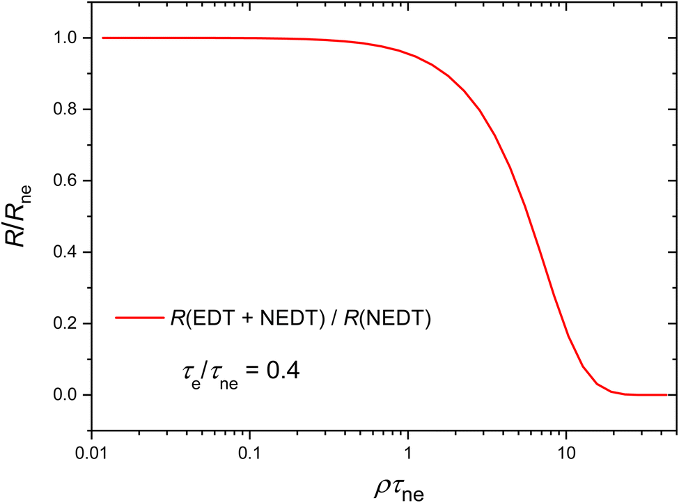Fig. 5 Ratio of the throughput formula for an EDT-NEDT cascade (eqn (3), for τ_e/τ_ne = 0.4) to that of a purely NEDT counter (eqn (2)), presented on a semi-logarithmic scale. The curve highlights the growing fraction of counts lost due to pulse pileup.

Inverse throughput

When observing a count rate R, inversion of the throughput formula is required to calculate a best estimate [small rho, Greek, circumflex] of the original input rate. In the case of NEDT, inversion of eqn (2) is easily achieved:¹⁶

Eqn (6) is commonly used in mass spectrometry to compensate for the main count loss component due to NEDT.

The case of EDT is less straightforward; the recursive relationship¹⁶

[small rho, Greek, circumflex]_< = Re^{[small rho, Greek, circumflex]τ_e} (7)

can be solved iteratively for [small rho, Greek, circumflex]_< ≤ 1/τ_e, using, for example, as a first approximation:

Another convenient approach for EDT is to use a series expansion:¹⁷

to obtain the solution for relatively low count rates, i.e. [small rho, Greek, circumflex]_< ≤ 1/τ_e. Since the throughput curve takes the shape of an asymmetric bell (Fig. 3), for each R value there are two solutions: one for ρτ_e ≤ 1 and a second for ρτ_e ≥ 1. The following series expansion is designed to obtain both solutions, [small rho, Greek, circumflex]_< and [small rho, Greek, circumflex]_>, by changing the sign in the formula:^17,28where and some numerical values of the coefficients c_j are provided in Refs. 17 and 28. To achieve the required precision, one can use the first values (c₀ = 1, c₁ = −1/3, c₂ = 1/36, c₃ = 1/270, c₄ = 1/4320) as a starting point in eqn (10), and then continue with a Newton–Raphson iteration:

Of particular interest to mass spectrometry is the inverse of the throughput formula in eqn (3), which relates to EDT and NEDT in series. This can be solved iteratively through the following recursion formula:^16,18

At moderate input rates (ρτ_e ≤ 1), eqn (6) can be applied as a first approximation for [small rho, Greek, circumflex] on the right-hand side of eqn (12), with an accurate result typically obtained after 1 to 3 iterations.

Since the throughput curve in Fig. 3 passes through a maximum, there are two possible solutions to the inversion of eqn (3): one for ρτ_e ≤ 1 and another for ρτ_e ≥ 1. Some elaborate inversion formulas have been derived by Libert.²⁹ In this work, a Newton–Raphson iteration method is proposed to find the solutions:

where z = e^{[small rho, Greek, circumflex]τ_e} + [small rho, Greek, circumflex](τ_ne−τ_e) and the starting value for the second solution ([small rho, Greek, circumflex] ≫ 1/τ_e) is inspired by a series expansion of the Lambert W function:

Convergence is typically achieved in a few iterations. Eqn (13) is also applicable at low count rates, where eqn (6) can be used for the starting value. The most challenging region lies near the maximum of the throughput curve, where the derivative approaches zero.

Pulse width and dead time

Best estimates of the pulse width and dead time can be obtained by conducting a linearity test at different input rates and using a least squares fitting procedure to identify the parameter values that optimally restore linearity.

An additional test can be considered by comparing two measurements with the same input rate, but different values of the NEDT: measurement 1 with the NEDT shorter than the pulse width, τ_ne < τ_e, and measurement 2 with a longer NEDT, τ_ne > τ_e. The first measurement is equivalent to an EDT counter with exponential throughput (eqn (1)), 1/R₁ = ρ⁻¹e^ρτ_e, whereas the second has an EDT-NEDT throughput (eqn (3)), 1/R₂ = ρ⁻¹e^ρτ_e + (τ_ne − τ_e). Then a simple relationship holds between the dead-time values and the inverse count rates:

If τ_ne > τ_e in both measurements, one obtains the difference between the NEDT values:

Live-time counting

There are more effective alternatives for compensating rate-related count loss than inverting the throughput curve. The simplest method of dead-time correction is “live-time counting”, which uses a live-time clock, where an accurately timed pulse train (“virtual pulser”) is counted only during the time intervals when the measuring system is free to accept or record events.^16,17 In this particular case, the dead-time region corresponds to a logical OR of the imposed NEDT and the pulse widths of all events, both “valid” and “invalid”. A schematic representation is shown in Fig. 6.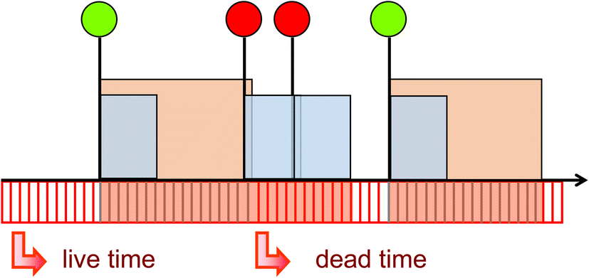

Fig. 6 Schematic representation of the logic used in an internal live-time clock, where a “virtual pulser” checks the availability of the counter to process pulses. The dead-time intervals encompass both the non-extending dead time and the duration of each pulse.

The live-time technique works effectively in a steady regime, for a so-called “stationary Poisson process”. The input rate can be calculated from the output rate by correcting with the ratio of real time (T_R = T_L + T_D) to live time (T_L):

Implementing this technique in mass spectrometry could resolve the dead-time issues to a satisfactory level, particularly when the input rate remains constant. In radionuclide metrology, additional measures are taken to correct for correlation effects between input rate and dead time, which mostly affect short-lived nuclides compared to long-lived ones. These corrections include formulas,^16,17,40 “loss-free counting” techniques^41–46 to manage rapidly varying dead times, and pileup-rejection mechanisms to avoid sum pulses that distort the energy spectrum.^38,39,47 Some of these measures may also be of interest to mass spectrometry, especially when analysing transient signals.

Uncertainty

The distribution of the number of events N recorded during a fixed-real-time measurement generally exhibits underdispersion relative to a Poisson process, resulting in a smaller standard deviation than the square root of N:^16,18

However, the variation in the dead-time corrected number of counts, N_c, is always overdispersed.¹⁶ The degree of overdispersion depends on the method used to compensate for dead time. The most accurate method involves a live-time counting technique, assuming a sufficiently long measurement time to accurately establish the correction factor T_R/T_L. The resulting relative uncertainty in the dead-time corrected number of counts is then (at least):

where X = R/ρ is the throughput factor from eqn (3).

In the less favourable case where no live-time information is available, the dead-time corrected counts must be calculated by inverting the throughput formula (eqn (12) or (13)), which introduces a higher variance. The resulting uncertainty equation is (Fig. 7):^16,18

Fig. 7 Uncertainty propagation factor (i.e., “overdispersion” relative to Poisson statistics, using eqn (20)) for the EDT-NEDT (τ_e/τ_ne = 0.4) corrected number of counts, derived from the inverse throughput formulas (eqn (12) or (13)).

The additional uncertainty factor in eqn (20) depends only on ρ and τ_e, not on τ_ne. Therefore, this type of uncertainty cannot be reduced by imposing a longer NEDT. Where the throughput formula in eqn (3) reaches a maximum, the uncertainty in eqn (20) approaches infinity. In this region, a more realistic uncertainty value can be estimated by performing the inversion for two different output rates, R_1,2 = R ± σ(R)/2. The input rate of the major isotope can also be verified by comparing it with the rate from a minor isotope with lower abundance and, consequently, lower count loss.

In addition to the count rate uncertainty, the uncertainty on the characteristic dead time parameters τ_ne and τ_e must be propagated into the uncertainty budget of the estimated input rate.¹⁶ The associated sensitivity factors are calculated from σ²(ρ) ≈ (∂R/∂ρ)⁻²(∂R/∂τ)²σ²(τ), which results in:

A graphical illustration is shown in Fig. 8 for τ_e/τ_ne = 0.4. At relatively low count rate (ρτ_e < 0.4), the propagation factor for NEDT is larger than for pileup and approximates the sensitivity factor ρτ_ne typical of a NEDT counter.¹⁶ Both sensitivity factors go well beyond unity at high input rates (ρτ_e > 0.5), where e.g. 1% error in pulse width can result in several % error in the estimated count rate. Uncertainty budgets that do not incorporate dead-time propagation may be severely incomplete.

Fig. 8 Propagation factor (eqn (21)) of relative uncertainty on the NEDT τ_ne and the pulse width τ_e with respect to the reverse throughput rate for sequential EDT-NEDT with τ_e/τ_ne = 0.4. A sensitivity factor of 1 translates a 1% error in τ_ne or τ_e into a 1% error in atomic abundance.

Amount ratio

The amount ratio of two isotopes, r = n₁/n₂, is assumed to be proportional to the intensities of their respective ion beams in the mass spectrometer, and thus also to the rate of ions impinging on the ion counter, r = ρ₁/ρ₂. Current practice involves calculating the ratio of the measured count rates, R₁ and R₂, corrected for the expected count loss due to NEDT only (eqn (8)). The approximate isotope ratio estimate is then:

However, an unbiased calculation of the isotope ratio should use the more complete throughput formula from eqn (3):

The error associated with the approximation in eqn (22) can be calculated as:

This error cancels out when both isotopes have equal concentrations, n₁/n₂ = ρ₁/ρ₂ = 1, and increases progressively as the isotope ratio moves away from unity.

Numerical example

Numerical examples are provided in Tables 1 and 2 and visualised in Fig. 9–11. An ion counter is modelled with a characteristic pulse width of τ_e = 20 ns and an imposed NEDT of τ_ne = 50 ns. The material consists of major and minor isotopes with an abundance ratio of n₁/n₂ = 30. Table 1 contains representative data regarding the expected count rates and throughput factors, before and after corrections for the count loss due to NEDT. Fig. 9 shows the corresponding throughput curves in a log–log scale. Mass spectrometry will result in biased atom ratios where the count rates for both isotopes are no longer parallel. Correcting for NEDT viaeqn (6) extends the linearity region by an order of magnitude. Linearity can be fully restored by using the inverse throughput formulas in eqn (12) and (13). Table 2 shows the results from the first iteration steps. The Newton–Raphson method (eqn (13)) converges faster and is applicable over the full range.

Table 1 Application of the throughput formula in eqn (3) for an ion counter with τ_e = 20 ns pulse width and τ_ne = 50 ns imposed non-extending dead time. Index 1 refers to the major isotope, and index 2 refers to a minor isotope with 30 times lower abundance in the material. The second half of the table shows count rates that have been partially compensated for count loss using the inverse throughput formula for NEDT in eqn (6)

Input		Uncorrected throughput					Corrected for NEDT
ρ 1 τ e	ρ 1	R 1	R 2	X 1	X 2	X 1/X2
0.0004	2 10^4	2.00 10^4	6.67 10^2	0.9990	1.0000	0.9990	2.00 10^4	6.67 10^2	1.0000	1.0000	1.0000
0.01	5 10^5	4.88 10^5	1.67 10^4	0.9756	0.9992	0.9764	5.00 10^5	1.67 10^4	0.9999	1.0000	0.9999
0.1	5 10^6	3.98 10^6	1.65 10^5	0.7967	0.9917	0.8033	4.97 10^6	1.67 10^5	0.9949	1.0000	0.9949
0.4	2 10^7	9.56 10^6	6.45 10^5	0.4781	0.9677	0.4940	1.83 10^7	6.67 10^5	0.9159	0.9999	0.9160
1	5 10^7	1.19 10^7	1.54 10^6	0.2371	0.9226	0.2570	2.91 10^7	1.67 10^6	0.5820	0.9994	0.5823
2	1 10^8	9.63 10^6	2.85 10^6	0.0963	0.8555	0.1125	1.86 10^7	3.33 10^6	0.1856	0.9977	0.1860
6	3 10^8	7.27 10^5	6.57 10^6	0.0024	0.6573	0.0037	7.55 10^5	9.79 10^6	0.0025	0.9790	0.0026

---

Table 2 Application of the inverse throughput formulas in eqn (12) and (13), showing the first iteration steps used to estimate the input rate ρ from the observed count rate R

Input		Eqn (12) with starting value from eqn (6)					Eqn (13) with starting values from eqn (6) or (14)
ρτ e	X	X ^(0)/X	X ^(1)/X	X ^(2)/X	X ^(3)/X	X ^(4)/X	X ^(0)/X	X ^(1)/X	X ^(2)/X	X ^(3)/X	X ^(4)/X
0.0004	0.9990	1.0000	1.0000	1.0000	1.0000	1.0000	1.0000	1.0000	1.0000	1.0000	1.0000
0.01	0.9756	0.9999	1.0000	1.0000	1.0000	1.0000	0.9999	1.0000	1.0000	1.0000	1.0000
0.1	0.7967	0.9949	0.9981	1.0000	1.0000	1.0000	0.9949	1.0000	1.0000	1.0000	1.0000
0.4	0.4781	0.9159	0.9338	0.9885	0.9979	0.9996	0.9159	0.9952	1.0000	1.0000	1.0000
1	0.2371	0.5820	0.5997	0.7111	0.7712	0.8096	1.8037	1.3052	1.1381	1.0660	1.0323
2	0.0963	0.1856	0.1892	0.2007	0.2027	0.2031	1.0735	1.0011	1.0000	1.0000	1.0000
6	0.0024	0.0025	0.0025	0.0025	0.0025	0.0025	0.9455	0.9938	0.9999	1.0000	1.0000

---

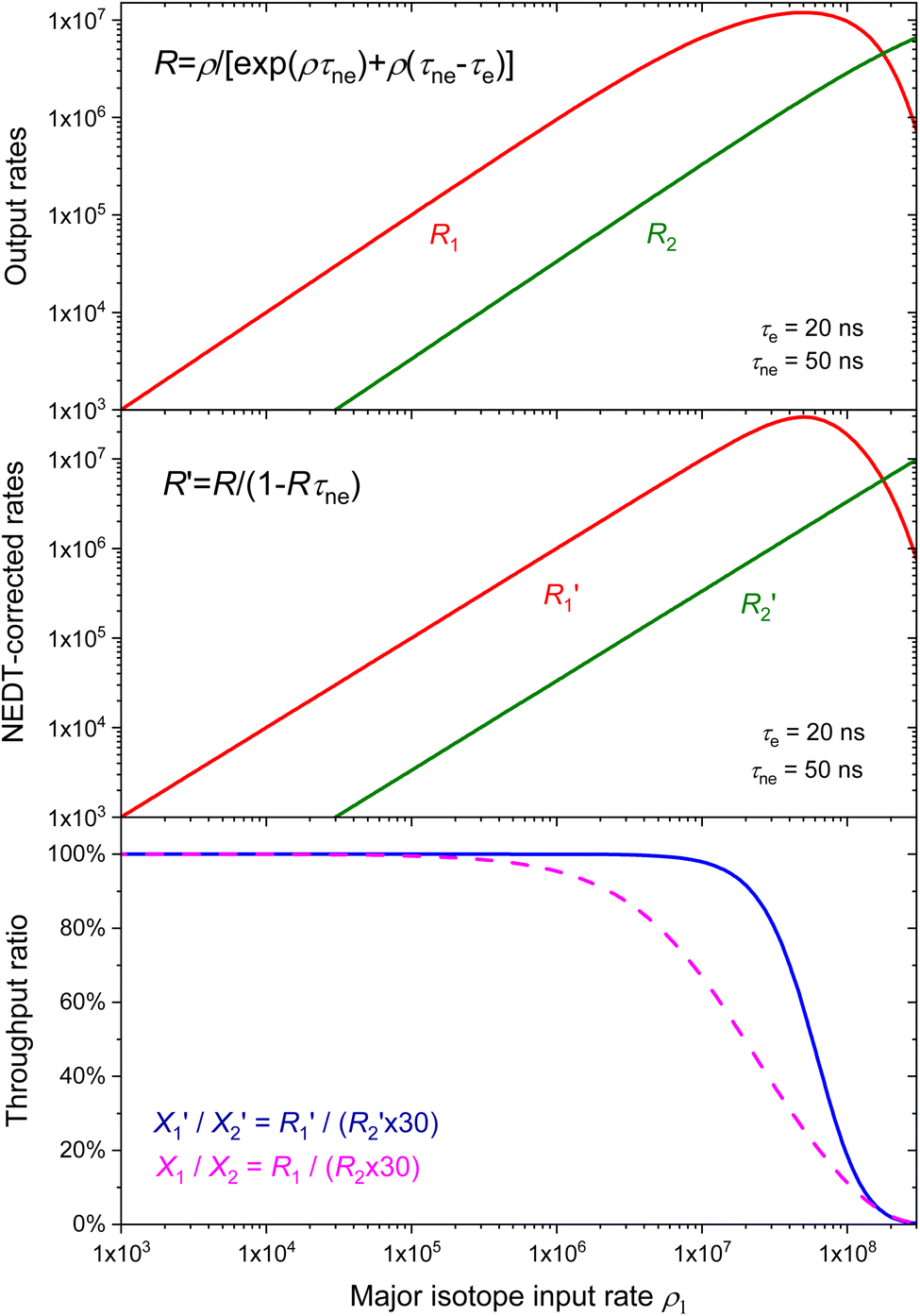Fig. 9 (Top) Output rate from an ion counter with τ_e = 20 ns and τ_ne = 50 ns for major and minor isotopes in a material with an atom ratio n₁/n₂ = 30, as a function of the major input rate. When both curves run in parallel, the mass spectrometry result is unbiased; (Middle) Same output rates after correction for NEDT using eqn (6). The linearity region has been extended by an order of magnitude; (Bottom) Throughput ratio for both isotopes, before and after NEDT correction. Deviation from unity indicates the non-linear working region of the mass spectrometer.

Fig. 10 The throughput ratio X₁/X₂ (before and after correction for NEDT) of the major and minor isotope as a function of the observed (non-corrected) count rate of the major isotope. There are two solutions, one for ρτ_e ≤ 1 and another for ρτ_e ≥ 1. At excessively high input rates, the experimenter may experience huge non-linearity effects.

Fig. 11 The throughput ratio X₁/X₂ (without NEDT correction) of the major isotope relative to minor isotopes, as a function of the observed (non-corrected) count rate of the major isotope. This ratio represents the bias observed in the measured atom ratios. The non-linearity effect increases with larger n₁/n₂ values.

Fig. 10 and 11 illustrate the non-linearity as a function of the output rate of the main isotope, which may be viewed as the experimenter's perspective. At high input rates (ρ₁τ_e ≈ 1), the user may observe quite excessive variations in the atomic ratio as a function of the output rate. Fig. 11 shows the throughput ratio for various atom ratios at typical output rates used in linearity tests. The graph reveals a rather flat region at low count rates, followed by a bend, and a sharp deviation from linearity. This pattern resembles experimental linearity plots published in literature, however the sign is opposite.^3,5

Experiment

Previous studies on ion counter linearity in mass spectrometry were generally limited to relatively low count rates (below 10⁻⁶ s⁻¹), where pulse pileup effects are minimal and difficult to measure accurately, but where other effects might cause apparent non-linearity, such as a high-frequency transient oscillations (“ringing”),⁴⁸ drift and aging effects,⁴⁹etc. Thus, linearity tests published in 2001 (ref. 3) and 2009 (ref. 5) show the opposite behaviour as expected from the throughput model. With increasing input rate, the output rate of the major isotope was higher than predicted from the NEDT model, resulting in seemingly lower isotopic abundances for the minor isotopes. One plausible explanation would be that excess counts were generated by afterpulses from multiple ions arriving at the detector in rapid succession. This can lead to amplifier-overload events, potentially causing a “ringing” effect in the electronic circuitry. The resulting electronic oscillations may generate spurious afterpulses that are erroneously counted as additional ions. These afterpulses would disproportionately affect the measurements of the most abundant isotope. Consequently, this would inflate the count rate for the major isotope relative to the minor isotopes, leading to an apparent decrease in the abundance of minor isotopes. This problem was eventually solved with the introduction of a new generation of SEMs with improved linearity via a lower operating voltage and modified last dynode electronics.^5,48

In 2016,⁷ static linearity tests were performed on a multi-collector inductively coupled plasma mass spectrometer (MC-ICP-MS) at the IAEA, using IRMM-072 reference material from the JRC. The results revealed that the dead-time effect aligned with that of a NEDT counter, and no additional count loss due to pileup was observed up to count rates of 8 10⁵ s⁻¹. While the observed dead time closely approximated the nominal value specified by the manufacturer, notable deviations up to about 3 ns were identified. Measurement of the dead time is therefore mandatory for accurate mass spectrometry. The authors posit that the dead time of any type of secondary electron multiplier detector is much shorter than the NEDT of τ_ne = 20–70 ns, possibly at the level of τ_e < 10 ns, and therefore can be disregarded as a source of count loss.

Within the framework of the throughput model presented in this work, the latter statement holds only partially true. Assuming an EDT-NEDT model with τ_ne = 20 ns and τ_e = 10 ns, the serial expansion of the throughput formula in eqn (5) can be further simplified to a first order approximation:

At an input rate of ρ = 10⁶ s⁻¹; the NEDT term is ρτ_ne = 0.02 and the EDT term is much smaller at just 0.00005. In this region, NEDT dominates and the pileup introduces only a minimal deviation of 0.005% to the count rate. Increasing the input rate by an order of magnitude to ρ = 10⁷ s⁻¹ leads to the respective terms of 0.2 for NEDT and 0.005 for EDT. At this rate, neglecting pileup introduces a significant error of 0.43% in X. This could be partially mitigated by adopting a slightly higher τ_ne value. At even higher count rates, accurate mass spectrometry results become unattainable within the NEDT model. For ρ = 10⁸ s⁻¹, the NEDT term is ρτ_ne = 2.0 and the sum of the pileup terms in eqn (5) amount up to 0.718, inducing 19% error on X.

In a recent study, Siegmund et al.⁵⁰ suggested an approach for investigating high intensity transient signals under controlled conditions by generating 200 μs ion beam pulses in MC-ICPMS with a liquid sample introduction to demonstrate the effect of intensity spikes that normally occur in laser ablation or nano-particle analysis. They performed a linearity test of secondary electron multipliers (SEM) subjected to a ²³³U/²³⁵U beam at input fluxes from ca. 10⁴ to about 3 × 10⁷ ions per second, and found that the investigated ion counters reveal some non-linearity beyond that caused solely by the dead time (whereas it was a valid approach for data acquired up to 2 × 10⁵ s⁻¹ ion count range). The diminishing response of the ion detection system at ion fluxes above 2 × 10⁶ s⁻¹ is compatible with additional count loss originating from pulse pile-up. In fact, the throughput curve up to 3 × 10⁷ s⁻¹ looks indeed as predicted in Fig. 3, and by applying the correction formula in eqn (12) they could fix the biased amount ratio. This is currently the most compelling direct evidence supporting the applicability of the model presented here to discrete ion counting in mass spectrometry. A more comprehensive experimental study is currently ongoing.⁵¹

For future tests, especially those involving transient signals, it is important to recognise a second, subtle form of non-linearity related to input rate variability. When the input rate varies significantly during measurement, an additional correction term must be included in the throughput formula to account for the non-proportionality between average input and output rates. This correction is proportional to the input rate variance and half the second derivative of the throughput function.⁵²

Conclusion

The presented throughput model predicts rate-related non-linearity in mass spectrometry when using a discrete ion counter. In current practice, count rates are corrected for count loss due to the imposed non-extended dead time, but not for the additional extending dead time generated by pileup of detector pulses. However, the NEDT model breaks down at extremely high count rates. Formulas have been provided for the true throughput rate (eqn (3)) in the counter, the inverse throughput to correct for count loss (eqn (6) and (12)–(14)), the resulting counting uncertainty (eqn (20)), the error propagation of the characteristic dead time and pulse width (eqn (21)), and the error made by incomplete dead-time correction when ignoring pileup (eqn (24)). As a result, this approach enables extending the linearity of the ion counter across the full range of input rates, thus eliminating rate-related bias in mass spectrometry.

Data availability

All data in Tables and graphs have been generated using the formulas presented in this paper.

Conflicts of interest

There are no conflicts of interest to declare.

Acknowledgements

Prof. Dr Oana-Alexandra Dumitru from the University of Florida is gratefully acknowledged for being a source of inspiration to accomplish this work.

References

1. N. S. Lloyd, J. Schwieters, M. S. A. Horstwood and R. R. Parrish, Particle detectors Used in Isotope Ratio Mass Spectrometry, with Applications in Geology, Environmental Science and Nuclear Forensics, in Handbook of Particle Detection and Imaging, ed. C. Grupen and I. Buvat, Springer-Verlag, Berlin Heidelberg, 2012.
2. A. Held and P. D. P. Taylor, A calculation method based on isotope ratios for the determination of dead time and its uncertainty in ICP-MS and application of the method to investigating some features of a continuous dynode multiplier, J. Anal. At. Spectrom., 1999, 14, 1075–1079.
3. S. Richter, S. A. Goldberg, P. B. Mason, A. J. Traina and J. B. Schwieters, Linearity tests for secondary electron multipliers used in isotope ratio mass spectrometry, Int. J. Mass Spectrom., 2001, 206, 105–127.
4. U. Nygren, H. Ramebäck, M. Berglund and D. C. Baxter, The importance of a correct dead time setting in isotope ratio mass spectrometry: Implementation of an electronically determined dead time to reduce measurement uncertainty, Int. J. Mass Spectrom., 2006, 257, 12–15.
5. S. Richter, A. Alonso, Y. Aregbe, R. Eykens, F. Kehoe, H. Kühn, N. Kivel, A. Verbruggen, R. Wellum and P. D. P. Taylor, A new series of uranium isotope reference materials for investigating the linearity of secondary electron multipliers in isotope mass spectrometry, Int. J. Mass Spectrom., 2009, 281, 115–125.
6. U. Nygren, H. Ramebäck, A. Vesterlund and M. Berglund, Consequences of and potential reasons for inadequate dead time measurements in isotope ratio mass spectrometry, Int. J. Mass Spectrom., 2011, 300, 21–25.
7. S. Richter, S. Konegger-Kappel, S. F. Boulyga, G. Stadelmann, A. Koepf and H. Siegmund, Linearity testing and dead-time determination for MC-ICP-MS ion counters using the IRMM-072 series of uranium isotope reference materials, J. Anal. At. Spectrom., 2016, 31, 1647–1657.
8. T. Hirata, S. Niki, S. Yamashita, H. Asanuma and H. Iwano, Uranium-lead isotopic analysis from transient signals using high-time resolution-multiple collector-ICP-MS (HTR-MC-ICP-MS), J. Anal. At. Spectrom., 2021, 36, 70–74.
9. I. Strenge and C. Engelhard, Single particle inductively coupled plasma mass spectrometry: investigating nonlinear response observed in pulse counting mode and extending the linear dynamic range by compensating for dead time related count losses on a microsecond timescale, J. Anal. At. Spectrom., 2020, 35, 84–99.
10. A. M. Duffin, E. D. Hoegg, R. I. Sumner, T. Cell, G. C. Eiden and L. S. Wood, Temporal analysis of ion arrival for particle quantification, J. Anal. At. Spectrom., 2021, 36, 133–141.
11. I. Strenge and C. Engelhard, Capabilities of fast data acquisition with microsecond time resolution in inductively coupled plasma mass spectrometry and identification of signal artifacts from millisecond dwell times during detection of single gold nanoparticles, J. Anal. At. Spectrom., 2016, 31, 135–144.
12. D. Mozhayeva and C. Engelhard, A critical review of single particle inductively coupled plasma mass spectrometry – A step towards an ideal method for nanomaterial characterization, J. Anal. At. Spectrom., 2020, 35, 1740–1783.
13. T. Hirata, S. Yamashita, M. Ishida and T. Suzuki, Analytical Capability of High-Time Resolution-Multiple Collector-Inductively Coupled Plasma-Mass Spectrometry for the Elemental and Isotopic Analysis of Metal Nanoparticles, Mass Spectrom. , 2020, 9, A0085.
14. S. Yamashita, M. Ishida, T. Suzuki, M. Nakazato and T. Hirata, Isotopic analysis of platinum from single nanoparticles using a high-time resolution multiple collector Inductively Coupled Plasma - Mass Spectroscopy, Spectrochim. Acta, Part B, 2020, 169, 105881.
15. S. Pommé, Radionuclide metrology: confidence in radioactivity measurements, J. Radioanal. Nucl. Chem., 2022, 331, 4771–4798.
16. S. Pommé, R. Fitzgerald and J. Keightley, Uncertainty of nuclear counting, Metrologia, 2015, 52, S3–S17.
17. International Commission on Radiation Units and Measurements (ICRU), Particle counting in radioactivity measurements, ICRU Report, Maryland, USA, 1994, vol. 52.
18. S. Pommé, Cascades of pile-up and dead time, Appl. Radiat. Isot., 2008, 66, 941–947.
19. S. Pommé, When the model doesn’t cover reality: examples from radionuclide metrology, Metrologia, 2016, 53, S55–S64.
20. J. A. Williamson, M. W. Kendall-Tobias, M. Buhl and M. Seibert, Statistical evaluation of dead time effects and pulse pileup in fast photon counting. Introduction of the sequential model, Anal. Chem., 1988, 60, 2198–2203.
21. R. Jakopič, K. Toth, J. Bauwens, R. Buják, C. Hennessy, F. Kehoe, U. Jacobsson, S. Richter and Y. Aregbe, 30 years of IRMM-1027 reference materials for fissile material accountancy and control: development, production and characterisation, J. Radioanal. Nucl. Chem., 2021, 330, 333–345.
22. S. Boulyga, S. Konegger-Kappel, S. Richter and L. Sangély, Mass spectrometric analysis for nuclear safeguards, J. Anal. At. Spectrom., 2015, 30, 1469–1489.
23. O. A. Dumitru, J. Austermann, V. J. Polyak, J. J. Fornós, Y. Asmerom, J. Ginés, A. Ginés and B. P. Onac, Constraints on global mean sea level during Pliocene warmth, Nature, 2019, 574, 233–236.
24. P. T. Spooner, T. Chen, L. F. Robinson and C. D. Coath, Rapid uranium-series age screening of carbonates by laser ablation mass spectrometry, Quat. Geochronol., 2016, 31, 28–39.
25. I. De Lotto, P. F. Manfredi and P. Principi, Counting statistics and dead-time losses, Energ. Nucl., 1964, 11, 599–611 ( Energ. Nucl. , 1964 , 11 , 557–564 ).
26. J. W. Müller, Sur l’arrangement en série de deux temps morts de types différents, Internal Report BIPM, Sèvres, France, BIPM-73/9, 1973.
27. J. W. Müller, Dead-time problems, Nucl. Instrum. Methods, 1973, 112, 47–57.
28. J. W. Müller, Stastiques de comptage, Internal Report BIPM, Sèvres, France, BIPM-82/13, 1982.
29. J. Libert, Détermination du taux de comptage en amont de deux temps morts classiques en série et de types différents, Nucl. Instrum. Methods Phys. Res., Sect. A, 1989, 274, 319–323.
30. S. Pommé, B. Denecke and J.-P. Alzetta, Influence of pileup rejection on nuclear counting, viewed from the time-domain perspective, Nucl. Instrum. Methods Phys. Res., Sect. A, 1999, 426, 564–582.
31. S. Pommé, Time-interval distributions and counting statistics with a non-paralysable spectrometer, Nucl. Instrum. Methods Phys. Res., Sect. A, 1999, 437, 481–489.
32. S. Pommé and G. Kennedy, Pulse loss and counting statistics with a digital spectrometer, Appl. Radiat. Isot., 2000, 52, 377–380.
33. S. Pommé and J. Uyttenhove, Statistical precision of high-rate spectrometry with a Wilkinson ADC, J. Radioanal. Nucl. Chem., 2001, 248, 263–266.
34. S. Pommé, Dead time, pile-up and counting statistics, in Applied Modeling and Computations in Nuclear Science, ACS Symposium Series, 2007, vol. 945, pp. 218–233.
35. S. Pommé and J. Keightley, Count rate estimation of a Poisson process - Unbiassed fit versus central moment analysis of time interval spectra. In: Applied Modeling and Computations in Nuclear Science, ACS Symp. Ser., 2007, 945, 316–334.
36. C. Michotte and M. Nonis, Experimental comparison of different dead-time correction techniques in single-channel counting experiments, Nucl. Instrum. Methods Phys. Res., Sect. A, 2008, 608, 163–168.
37. S. Cheng, B. Pierson, S. Pommé and M. Flaska, Time interval distributions of nuclear events in a digital spectrometer, Nucl. Instrum. Methods Phys. Res., Sect. A, 2024, 1063, 169218.
38. S. Pommé and K. Pelczar, A simplified approach to counting statistics with an imperfect pileup rejector, Nucl. Instrum. Methods Phys. Res., Sect. A, 2025, 1070, 170067.
39. S. Cheng, B. Pierson, S. Pommé, B. Archambault and M. Flaska, Time-interval distributions in a digital gamma multi-channel analyzer at extreme input rates, Nucl. Instrum. Methods Phys. Res., Sect. A, 2025, 1073, 170260.
40. R. Fitzgerald, Corrections for the combined effects of decay and dead time in live-timed counting of short-lived radionuclides, Appl. Radiat. Isot., 2016, 109, 335–340.
41. G. P. Westphal, Review of loss-free counting in nuclear spectroscopy, J. Radioanal. Nucl. Chem., 2008, 275, 677–685.
42. S. Pommé, J.-P. Alzetta, J. Uyttenhove, B. Denecke, G. Arana and P. Robouch, Accuracy and precision of loss-free counting in γ-ray spectrometry, Nucl. Instrum. Methods Phys. Res., Sect. A, 1999, 422, 388–394.
43. S. Pommé, How pileup rejection affects the precision of loss-free counting, Nucl. Instrum. Methods Phys. Res., Sect. A, 1999, 432, 456–470.
44. S. Pommé, Experimental test of the 'zero dead time' count-loss correction method on a digital gamma-ray spectrometer, Nucl. Instrum. Methods Phys. Res., Sect. A, 2001, 474, 245–252.
45. S. Pommé, A plausible mathematical interpretation of the 'variance' spectra obtained with the DSPECPLUS TM digital spectrometer, Nucl. Instrum. Methods Phys. Res., Sect. A, 2002, 482, 565–566.
46. S. Pommé, On the statistical control of 'loss-free counting' and 'zero dead time' spectrometry, J. Radioanal. Nucl. Chem., 2003, 257, 463–466.
47. J. Bartošek, J. Mašek, F. Adams and J. Hoste, The use of a pileup rejector in quantitative pulse spectrometry, Nucl. Instrum. Methods, 1972, 104, 221–223.
48. S. R. Noble, J. Schwieters, D. J. Condon, Q. G. Crowley, N. Quaas and R. R. Parish, TIMS Characterization of a New Generation Secondary Electron Multiplier, AGU Fall Meeting, 2006, session V11E-06.
49. P. M. L. Hedberg, P. Peres, F. Fernandes and L. Renaud, Multiple ion counting measurement strategies by SIMS– a case study from nuclear safeguards and forensics, J. Anal. At. Spectrom., 2015, 30, 2516–2524.
50. H. Siegmund, S. Konegger-Kappel and S. Boulyga, Analysis of ultra-fast transient signals by LA-MC-ICPMS – overcoming instrumental limitations, European Workshop on Laser Ablation, Ghent, Belgium, 2024.
51. H. Siegmund, S. Konegger-Kappel, S. Boulyga, M. Kilburn and S. Pommé, Recording High-Intensity Transient Signals with Secondary Electron Multipliers in MC-ICPMS: Dead-Time Correction and Non-linearity Effects, 2025, in preparation.
52. S. Pommé, Non-linearity correction for variable signal analysis in mass spectrometry using discrete ion counters, 2025, in preparation.

---