Unveiling the impact of ligand configurations and structural fluxionality on virtual screening of transition-metal complexes

Abstract

Computational exploration of chemical space is a powerful tool for designing organometallic homogeneous catalysts. While catalytic properties depend on ligand properties and spatial arrangement, the role of stereoisomerism in defining catalyst selectivity and reactivity has only been elucidated sporadically, leaving gaps in virtual screening workflows. This study investigates the necessity of exploring ligand configurations for virtual high-throughput (HT) screening of octahedral transition metal complexes. Using automated workflows, ligand configuration ensembles were generated for bisphosphine ligands with Ir(III), Ru(II), and Mn(I) metal centers. DFT calculations revealed distinct preferences for Ir(III) configurations, whereas Mn(I)- and Ru(II)-complexes displayed significant fluxionality, with multiple configurations within a 10 kJ mol⁻¹ energy range. Linear regression analyses showed that global descriptors, such as bite angle and HOMO–LUMO gap, are transferable across configurations and metal centers, while local steric descriptors lacked such transferability. Machine learning (ML) models successfully classified ligand configurations (balanced accuracy >0.8) but struggled to predict stability across metal centers, especially for Mn(I) and Ru(II). Thus, improved descriptors of the first coordination sphere to capture fluxionality and stability more effectively can improve ML models. Overall, this study underscores the limitations of ignoring stereoisomerism in virtual HT screening, which may lead to incomplete exploration of chemical space and underrepresentation of key catalyst features. Until dynamic digital representations are developed, exhaustive stereoisomerism exploration should be implemented for screening workflows.

---

1 Introduction

Homogeneous catalysis serves as the enabling technology for numerous organic chemical transformations.^1–3 The production of stereospecific compounds requires high precision, for which an important and versatile class of homogeneous catalysts consists of organometallic complexes with tunable ligands.^4,5 Due to the relatively well defined design space, for example, the denticity of ligands and oxidation states of metal centers, computational catalyst design may seem trivial. However, the nearly endless possibilities of metal–ligand combinations make exploration of the chemical space a challenge.^6–9 Fortunately, many methods have been developed that help navigate this multidimensional space. Commonly employed approaches involve virtual high-throughput (HT) screening,^10–15 generative models¹⁶ and combinatorial chemistry.^12,17,18 Virtual screening of the metal–ligand space has been enabled by several (semi-)automated workflows utilizing data-driven quantitative structure activity/selectivity relationships (QSAR/QSSR).^19–25 These methods often consist of a workflow comprising four fundamental components: structure generation, electronic structure calculation, descriptor extraction and finally statistical modeling to relate descriptors to catalyst behavior.^26,27

Generally, these workflows start with assumptions based on a specific reaction mechanism.¹³ Considering the flexibility of these ligands, one thus assumes that a preferred ligand arrangement is retained for all members of a given ligand family and/or metal centers. Conformational search aiming at identifying low-energy rotamers and isomeric structures is commonly carried out for this selected coordination polyhedron with the pre-defined ligand configuration, which is preserved at this stage.^28,29 Although the kinetic trans-/cis-effect is well known,³⁰ the role of stereoisomerism of the catalyst in defining selectivity and reactivity has only been elucidated sporadically.^31–33

The relationship between the stability and observed catalytic properties of a complex is challenging to comprehend and is usually not known a priori. Consider a scenario where a meta-stable configuration of a TM complex, existing at a low concentration in the reactive system, establishes a favorable reaction channel. This minor catalytic component would provide a major impact on the reaction rate and would therefore determine the nature and characteristics of the primary reaction product (Fig. 1).^34–40 As an example, two possible ligand arrangements are depicted in Fig. 1a and b. Although complexes with a different ligand configuration are in equilibrium, one meta-stable configuration may provide a reaction path with an energy barrier that is significantly higher than that of the other configuration. The overall ensemble of ligand configurations ultimately contributes to the observed catalytic properties. In the context of virtual HT screening, the conformational isomerism of the organic ligand backbone has been recognized by the community^27,41–43 and various structure generation tools such as AARON, Architector, Molsimplify, Molassembler and AQME, contain on-the-fly conformer generation solutions.^44–48 However, due to the initial selection of a configuration, the influence and contribution of the metastable configurations featuring varied coordination environments and ligand arrangements might be overlooked. Furthermore, this choice assumes that the preferred configuration does not change with relatively minor variations in the ligand structure and, often, even the nature of the metal center. Consequently, the question arises: can catalytic systems be fully accounted for when part of the chemical space is neglected due to initial human choices and intuition in structure generation?

Fig. 1 Selectivity control by minor configurations: schematic representation of the impact of a minor (a) and major (b) isomer of a TM complex on the reactivity and selectivity in chemical transformations.

To investigate this, we focused on TM-complexes that are relevant to homogeneous catalysis for hydrogenation reactions, where bidentate ligands are commonly employed to achieve high reactivity and enantioselectivity.^49–52 To ensure that the generated data is as bias-free and comprehensive as possible, we employed an automated workflow for construction, sorting and descriptor calculation of ensembles of ligand configurations for TM-complexes. We constructed ensembles containing different ligand configurations for 87 bidentate ligands connected to 3 different metal centers, namely Ir(III), Ru(II) and Mn(I), yielding a total of 908 octahedral TM-complexes. With these data, we set out to model the relations between stereoisomerism, stability, and descriptors.

The primary research question of this work is whether an exhaustive exploration of stereoisomerism is necessitated for virtual HT screening of octahedral TM-based catalyst complexes, given that the degree of configurational fluxionality of a complex is not fully known a priori. To answer this, we investigated whether specific ligand configurations of the TM-complexes proved to be more energetically favorable and whether this could be modeled using physical–chemical descriptors and machine learning (ML). The paper is organized as follows. Initially, stability trends of different ligand configurations were analyzed on the basis of results from Density Functional Theory (DFT) calculations. The results were analyzed by means of linear regressions to identify relevant descriptors across different ligand configurations and metal centers. The descriptors were then utilized to construct ML models capable of distinguishing different types of ligand configurations and predicting energetic preferences for specific metal–ligand combinations. Our results highlight the challenge of configurational fluxionality for the virtual screening of TM complexes and provide practical directions to address them.

2 Methods

2.1 Ligands and transition metal complexes

The investigated TM-complexes employed various bidentate ligands with isoelectronic Ir(III), Ru(II) and Mn(I) metal centers. The selected auxiliary ligands, next to the bidentate ligands, were hydrides and CO such that neutral TM-complexes were generated. Importantly, all complexes in this study were treated in their closed-shell singlet (i.e., diamagnetic) configurations. In particular, Mn(I) complexes with strong-field ligands such as CO are known to favor low-spin electronic configurations due to the large ligand field splitting they induce, consistent with their position on the spectrochemical series.^53,54 Acetonitrile served as a model substrate to ensure minor impact on the overall conformational freedom of the complexes. More specifically, we have explored the configurational freedom and physical–chemical properties of an extended catalyst dataset featuring 87 chiral bisphosphine (PP) ligands coordinated to neutral transition-metal complexes. To maintain charge neutrality, Ir(III), Ru(II), and Mn(I) centers were stabilized with different auxiliary ligands, resulting in PPIrH₃(CH₃CN), PPRuH₂(CO)(CH₃CN), and PPMnH(CO)₂(CH₃CN) complexes, respectively. The dataset was constructed without any a priori assumption of the preferred ligand arrangement or TM stereochemistry using a fully automated workflow for the generation of TM complexes.⁵⁵ Fig. 2a illustrates the studied ligand configurations for the Ir, Ru and Mn complexes. The 87 selected bidentate PP ligands belong to different ligand families, a subset of which is shown in Fig. 2b. The complete set of bidentate ligands is available in the ESI† (see Data availability statement).

Fig. 2 (a) List of possible ligand configurations for each metal center (b) a selection of representative studied bisphosphine bidentate ligand families and (c) a selection of geometric, steric and electronic descriptors used in this study.

2.2 Complex generation and sorting workflow

The general workflow for generating and sorting TM-complexes as employed in this study is visualized in Fig. 3. Structures for TM-complexes were generated using the in-house Open Bidentate Ligand Explorer (OBeLiX) workflow (see Data availability statement).²⁷ This workflow aims to aid computational exploration of the organometallic chemistry space through automated structure generation and descriptor calculation. OBeLiX utilizes the MACE python package for the automated generation of 3D structures and stereochemistry assessment of TM-complexes.^55,56 MACE is an open source python package, which allows bias-free generation of 3D TM-complexes starting from molecular SMILES strings⁵⁷ of ligands and metal centers. Furthermore, MACE generates all possible stereoisomers, explores conformations and filters out identical and “impossible” sterically hindered configurations for the given metal–ligand combination. In this study, 50 conformers were generated using the universal force field as implemented in the RDKit package through MACE.

Fig. 3 Workflow for generating & sorting TM-complex geometries from specified user input.

After generating the structures for the TM-complexes via MACE, the complexes were named according to the first donor atoms axially bonded to the metal center as illustrated in Fig. 2. These axial ligand configurations were identified using bite angles. The coordinate system of TM-complexes are defined with respect to the bidentate ligand, and hence the bidentate ligand is always present in the equatorial position. Therefore, the ligands in the axial position are the only non-bidentate ligand containing pair forming a bite angle of 180°. For ligands lacking C₂ symmetry, variations arising from asymmetric functionalization on the phosphine donor atoms were treated as distinct conformers within the same axial ligand configuration. After generating and sorting the TM-complexes, geometries were optimized at the DFT level of theory.

2.3 Density functional theory calculations

The generated geometries were further refined by DFT calculations using Gaussian 16 C.02 (ref. 58) software. For geometry optimizations, the PBE0 (ref. 59) exchange–correlation functional was used with Grimme's DFT-D3(BJ) dispersion corrections⁶⁰ and the def2-SVPP basis set.⁶¹ The selected combination of basis set and exchange correlation functional have previously been established to generate reasonable energies and structures for similar TM-based complexes.^49,62–65 Normal mode analysis was carried out to confirm that the optimized geometries correspond to local minima on the potential energy surface. For structures with imaginary frequencies, the PyQRC python package^66,67 was used to remove these imaginary frequencies and restart geometry optimizations. After geometry optimization, energies were refined with single point (SP) calculations at the PBE0-D3 level using the def2-TZVPP basis set.^61,68

Thermodynamic stabilities of ligand configurations were calculated by the difference in the DFT-based electronic energies with respect to a reference configuration. The H–N axial ligand pair structure is used as the reference, being the only common configuration present among studied metal centers. The difference in stability between the reference and alternative configurations is denoted as ΔE_ref.

In addition to screening the stability of the TM-complexes, a screening based on substrate binding energy was also conducted. Binding energies of the model substrate, acetonitrile, were computed as follows:

E_bind = E_DFT,complex − (E_{DFT,complex-nosub} + E_DFT,sub) (1)

In this equation, substrate binding energy is described by the DFT optimized energy differences between the complex, (E_DFT,complex) minus the sum of substrate-removed complex (E_{DFT,complex-nosub}) and the energy of non-bonded substrate (E_DFT,sub). More information about this screening approach can be found in ESI Sections S1 and S2.†

2.4 Descriptor calculation

The OBeLiX descriptor calculator²⁷ was employed to automate the extraction of chemical–physical properties and descriptors of DFT-optimized complexes. This tool determines electronic, steric and geometric descriptors using Morfeus⁶⁹ and cclib.⁷⁰ A graph-based method is employed to locate and label the bidentate donor atoms based on charges calculated by a xTB single-point calculation. Based on these charges, the donor atoms in the bidentate ligand are labeled as either ‘min’ or ‘max’. The structural and electronic descriptors were calculated on DFT-optimized structures. In total, 27 commonly used DFT-based descriptors were selected for the analysis (see descriptors overview in the ESI†).

2.5 Linear regression

These descriptors were utilized for linear regression to model relationships between descriptors across different ligand configurations and metal centers. The Scikit-learn Python package with default settings was used, hence the coefficient of determination was used as a scoring function for performance.

2.6 Machine learning

The calculated descriptors were also used in two ML modeling tasks: distinguishing different types of ligand configurations and predicting energetic preferences for specific metal–ligand combinations. The approaches leveraged a modified ML pipeline, adapted from our earlier work.⁴⁹ The first task was multi-class classification of configurations in which the TM-complexes were represented as a vector of descriptors and the target value was the axial pair of ligands, e.g. H–H and H–N for Ir-based complexes. This task was performed in two ways: (1) over the whole dataset containing all metal centers and ligand configurations or (2) divided per metal center. This enables highlighting of performance differences between TM-complexes and their respective metal centers. Additionally, the train/test split was done in two ways: (1) in-domain, in which the dataset was randomly divided into train- and test-set or (2) out-of-domain, in which a fixed set of 16 ligands and their configurations were kept out of the training set. This enables insights into the modeling performance on completely new ligands. In the second task, ML was employed for binary classification to model energetic preferences in ligand configurations. In this case the most stable configurations within a specific metal–ligand combination, would get a label 1, while the rest of the configurations for that combination would get a label 0. Again, this task was performed over either the whole dataset of all metal centers and ligand configurations or divided per metal center. The train/test split was also performed either in-domain or out-of-domain (vide supra).

The random forest (RF) and logistic regression (LR) algorithms were used. RF is an ensemble learning algorithm harnessing multiple decision trees and randomness to construct a predictive model, while logistic regression is a statistical method that models the probability of a binary outcome using a logistic function. In our study, all modeling tasks were attempted with both RF and logistic regression, with logistic regression serving as a simpler alternative to RF. The modeling tasks were evaluated with a balanced accuracy (BA) score which is a metric for evaluating classification models on imbalanced datasets. The score was calculated as follows:

Details about cross-validation, hyperparameter optimization and model initialization can be found in the ESI Section S3.†

3 Results and discussion

To explore the role of structural fluxionality in the in silico screening of catalyst complexes and to assess whether trends in the energetic landscape could be visually discerned or systematically predicted using machine learning (ML), the research was structured into four key steps: (1) a detailed analysis of the DFT-calculated energetic landscape of ligand configurations to identify trends and patterns across different metal centers, (2) statistical and linear regression analyses to examine the sensitivity of descriptors and their influence for combinations of specific configurations and metal centers, (3) ML-based classification to predict ligand configurations using these descriptors, and (4) ML-based classification to identify the most stable configuration for various ligand–metal center combinations.

3.1 Energetic preferences in ligand configuration

To investigate whether a specific configuration is generally more favorable compared to others, i.e. a global minimum on the Potential Energy Surface (PES), the relative stability of possible complex configurations is analyzed across our selection of bidentate bisphosphine ligands. The relative stability of alternative configurations with respect to the selected reference structure per metal center is presented in Fig. 4. At the top of each figure, the reference structure is depicted, with the alternative configurations shown at the bottom.

Fig. 4 Relative stability of ligand configurations, shown at the bottom of a graph, and a reference structure, shown at the top of a graph, for set of bidentate ligands for (a) Ir(III), (b) Ru(II) and (c) Mn(I) complexes.

The results for Ir(III) complexes (Fig. 4a) reveal that for most ligands the reference N–H axial ligand pair is more stable than the alternative H–H arrangement. In the case of Ru(II) (Fig. 4b), the presence of additional auxiliary ligands expands the configurational space, which now includes C–N, C–H and H–H as alternative axial ligand pairs next to the reference H–N. Upon assumption that hydrides are indistinguishable, Ir(III) complexes can only form two distinctive configurations, whereas four different configurations of the Ru complex can be formed. A significant variety in the data set is observed, as the complex configuration with the lowest stability often varies among the different bidentate ligands.

Similar to Ir(III), the H–H axial ligand configuration exhibits a positive ΔE_ref for the majority of bidentate ligands, signifying a lower stability compared to the reference H–N configuration. However, a notable difference from Ir(III) complexes is that alternative configurations exhibit higher stability for many systems. For instance, the C–N axial configuration commonly exhibits a negative ΔE_ref, indicating their higher stability than the H–N reference. Furthermore, our workflow identifies multiple Ru complexes with alternative configurations varying more than 50 kJ mol⁻¹ compared to the reference case. These outliers are the result of unfavorable conformations imposed by the specific ligand arrangement on the metal center. In particular, 6 ligands were identified as outlier for multiple metal centers (L86, L87, L119, L134 and L171), but no noteworthy trends were observed. Data on these outliers are contained in the data_analysis and descriptor_analysis directory in the ESI.†

A similar analysis for Mn(I) complexes (Fig. 4) reveals that the most stable preferred configuration varies between different bidentate ligands. Distinctive to Mn(I) complexes is the C–C configuration which shows a lower overall stability for most ligands. Nevertheless, as opposed to Ir(III) complexes, the reference H–N axial ligand configuration is not shown to be the most stable configuration in all cases. Instead, the C–H and C–N configurations are energetically more favorable.

Fig. 5 summarizes the axial ligand configurations along with the percentage of bidentate ligands for which those specific configurations are found to be the global minimum on the PES. For the Ir(III) complexes 92% of bidentate ligands show a clear global minimum in energy for the H–N configuration. The remaining 8% favor the single alternative H–H configuration. For Ru(II) complexes, the H–N axial configuration is also frequently identified as the global minimum, but this now only accounts for 50% of the bidentate ligands. Both the C–N and C–H axial ligand configurations emerge as the global minimum for a notable number of bidentate ligands, 31% and 18% respectively. The H–H axial ligand configuration is the global minimum for a single bidentate ligand. Unlike Ru(II) and Ir(III), related Mn(I) complexes do not display a pronounced majority of minima containing the H–N configuration. This geometry is preferred for only 26% of Mn(I) complexes, while the alternative C–H configuration is the global minimum for 45% of the bidentate ligands in this case. The C–N and C–C axial arrangement are preferred by 24% and 5% of the Mn(I) complexes respectively. These findings underscore that even though bidentate bisphosphine ligands are studied exclusively, no clear trend in the stability of a ligand configuration can be observed across the studied metal centers.

Fig. 5 Distribution of most stable ligand configuration over all possible ligand configurations for Mn(I), Ru(II) and Ir(III) complexes, alongside 87 bisphosphine (PP) bidentate ligands.

3.2 Transferability of descriptors to different ligand configurations and metal centers

Next, a statistical analysis of different physical–chemical descriptors was performed to identify relevant descriptors that are affected by changes in the configurations of various metal–ligand combinations. In total, a selection of 8 electronic, 4 geometric and 15 steric descriptors are considered in this study. Examples that will be discussed in more detail in this work are: the buried volume which comprises a measure of the steric occupation of a ligand, the NBO charges of the bidentate ligand's donor atoms and metal center in the TM-complex, the bite angle between metal center and bidentate ligand's donor atoms and finally the HOMO–LUMO gap. These descriptors are commonly utilized in studies of the reactivity and selectivity of homogeneous catalysts. In previous research, we have elucidated the relation between conformational flexibility and physical–chemical descriptors.⁷¹ We now focus on the transferability of descriptors between different configurations, metal centers and combinations thereof. Transferability in this context, thus, means that a descriptor can be reliably predicted from a selected configuration of a metal–ligand combination, from which it can be inferred which descriptors are sensitive to variations in stereoisomerism.

Linear regression models were constructed to predict specific descriptors of the complexes across different combinations of metals and ligand configurations. The models are scored using a coefficient of determination (R²) ranging from 0 to 1. Since there are 10 possible metal and ligand configuration combinations, the performance of (10 × 10) − 10 = 90 distinct linear models per descriptor is reported. Fig. 6 shows a heatmap for four selected descriptors and the resulting R² for the 100 models, the steric descriptors are depicted on the left and the electronic descriptors on the right. The top two descriptors in the figure represent local properties of the bidentate ligand, while the bottom two are more global. Each heatmap shows all possible ‘metal, configuration’ combinations on the x- and y-axes. Similar heatmaps for all calculated descriptors are provided in the ESI (Section S4†).

Fig. 6 Matrices for R² scores of linear models between specific descriptor from one set of bidentate ligands with a specific metal and ligand configuration to another set with a different combination of metal and ligand configuration. An example is shown for four selected descriptors that range in locality. An image for matrices of all calculated descriptors can be found in the ESI Section S4.†

Fig. 6 reveals a clear distinction in the transferability of the steric descriptors. The calculated physical–chemical descriptors differ in the level of locality that is captured, where a buried volume can be separated into quadrant- and octant-based contributions which offer a local view on the steric occupancy of a ligand, the bite angle remains a more global geometric measure. Although a local octant of the buried volume shows a low R² (R² < 0.5) for models across all metal and ligand configuration combinations, the bite angle shows a relatively high R² (R² > 0.7) across all metal and ligand configuration combinations. This is in line with the inherent low variance (33.5°) of the bite angle across the whole dataset. Similar observations are made and reported in the ESI Section S4† for the percentage buried volume with a radius of 3.5 at the metal center or ligand donor atoms.

For the electronic descriptors shown on the right in Fig. 6, the distinction in transferability is less pronounced. This is evidenced by the presence of red regions in the heatmap of the NBO charge, which deviates from the uniform blue observed in the local steric descriptors. The NBO charge at an atom describes the local electronic environment of the specified atom, while the HOMO–LUMO gap remains a global descriptor depicting the difference in energy of the frontier orbitals of the whole complex. The NBO charge at the ligand donor atom labeled ‘max’ shows varying modeling performance. Starting at the top left of the heatmap, the ‘Ir, H–H’ metal and configuration combination shows no transferability across any other combination. The ‘Ir H–N’ metal and configuration combination shows moderate R² (R² ≈ 0.6) for Ru(II)-based C–N and H–N configurations while a low R² is observed for all other combinations. On the bottom right, the Ru(II)-based configurations show a relatively moderate to high R² across other Ru(II)-based configurations. For Mn(I)-based configurations, the trend differs, as moderate to high R² values are observed only between the C–C, C–H, and C–N configurations. This highlights the sensitivity of certain descriptors to stereoisomerism and the nature of the metal center in the TM complex. In contrast, the HOMO–LUMO gap consistently exhibits high R² values (R² > 0.7) across all metal and ligand configuration combinations. Although the HOMO–LUMO gap itself seems transferable across metal and ligand configuration combinations, visualization of the frontier orbitals showed that the nature of the respective frontier orbitals may substantially differ with varied configurations. This analysis can be found in the ESI Section S5.†

3.3 ML modeling of ligand configurations

Given that certain descriptors are sensitive to changes in stereoisomerism and the nature of the metal center, the focus now shifts to the use of machine learning models to classify and predict the stability of ligand configurations based on these descriptors. Before applying this modeling approach, it is first necessary to assess the ability of machine learning to leverage the selected descriptors to distinguish between different ligand configurations. A comprehensive classifier was trained for either the whole dataset comprising all ligands and metals or metal-specific by dividing the dataset metal-wise. This leads to a five-class classification for the axial ligand pairs using either random forest or logistic regression algorithms.

The performance evaluation is shown in Fig. 7, where the x-axis depicts whether modeling was performed on the dataset comprising all metals or by metal-specific division. The BA on the test set for RF and LR are shown by a red and blue bar respectively. The modeling on the dataset containing all ligands, metals and ligand configurations reveals a gap in performance between the non-linear RF and the linear LR models. Where the RF models yielded a remarkable BA of 0.87–0.89, the LR models yielded a good BA of 0.73–0.79. Inspecting the performance of metal-specific models going towards the right in the figure, it can be observed that although all models perform good to excellent, a drop in performance is observed for Mn(I)-specific modeling. Nevertheless, these results suggest that the descriptors employed allow ML to effectively distinguish between different axial configurations. This holds true even for out-of-domain modeling cases where 16 ligands were kept out of the training set, simulating a case of applying the trained models to fully new ligands. The out-of-domain modeling results are contained in ESI Section S7.†

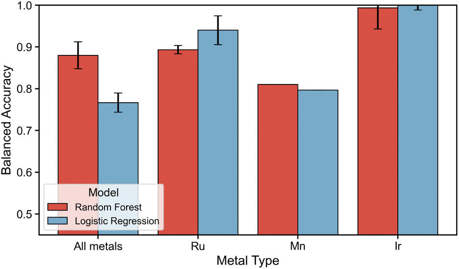Fig. 7 Performance metrics for the in-domain modeling of ligand configurations. The performance of RF and LR are displayed in a red and blue bar respectively. The y-axis denotes the balanced accuracy score and the x-axis specifies whether modeling is done on the dataset containing all metal centers and ligand configurations or on a metal-specific subset.

An examination of the feature importances (see ESI Section S6†) revealed that for modeling over all metal centers, descriptors such as the dipole moment, NBO charges on the metal or bidentate ligand donor atoms, and distances between the donor atoms and the metal center are of the highest importance. Thus, these importances reveal that the polarity of the complex (dipole moment) and the local electronic environment surrounding the metal and ligand donor atoms (all other mentioned descriptors) are informative enough to distinguish different ligand configurations for ML. This is in line with our findings on the transferability of descriptors, where those same descriptors are observed to exhibit a high sensitivity to changes in ligand configuration and metal center. However, it should be noted that an important difference is observed in the feature importances of Mn(I)-specific models. Where high importance is given in Ru(II)- and Ir(III)-specific models to the dipole moment and afterwards mainly descriptors of the local electronic environment surrounding the metal center, these seem of relatively lower importance in Mn(I)-specific models. Here, a higher importance is observed for more global descriptors such as the bite angle, cone angle and HOMO–LUMO gap. This observation points at a difference in which ML is able to distinguish ligand configurations of 3d TM-complexes compared to their 4d counterparts and is indicative of the gap in performance of Mn(I)-specific models compared to Ru(II)- and Ir(III)-specific models.

3.4 Thermodynamic accessibility of metastable configurations and ML modeling of energetic stability

Knowing that ML has the ability to distinguish different ligand configurations based on the given set of descriptors, we set out to model the stability of ligand configurations. However, the results in Fig. 4, reveal that multiple isomers of the same metal–ligand pair can exhibit similar stability. This finding suggests that, under the reaction conditions, multiple ligand configurations may contribute to the population of the coordination complex, thereby impacting the overall observed catalytic behavior. To quantitatively assess this factor, we have analyzed the proportion of systems for which multiple ligand configurations were obtained within an energy threshold of 10 kJ mol⁻¹ from the global minimum state. The choice of the 10 kJ mol⁻¹ threshold is based on the assumption that a catalyst population follows a Boltzmann average, resulting in at least 5%, and up to 50% of the total population to be in a metastable state under the reaction conditions commonly employed in homogeneous catalysis. For each ensemble of configurations, the number of configurations within a 10 kJ mol⁻¹ range of the lowest-energy isomer is obtained.

Fig. 8a reports the number of ligand configurations within the 10 kJ mol⁻¹ energy range from the most stable configuration for the Ir(III), Ru(II) and Mn(I) complexes, while the fraction of the respective complexes featuring multiple ligand configurations within this energy range is given in Fig. 8b. For the majority of Ir(III) complexes, only a single configuration is observed within the specified energy range. This finding is in line with the significant stability differences and small number of available ligand configurations. However, even in this case, 24% of Ir(III) complexes are expected to exhibit substantial structural isomerism, i.e. present multiple ligand configurations with stability difference <10 kJ mol⁻¹, under the reaction conditions. The fraction of such systems is much higher for Ru(II) and Mn(I) complexes, where multiple ligand configurations within 10 kJ mol⁻¹ stability range were found for 72% and 68% of the cases, respectively.

Fig. 8 (a) Number of ligand configurations within 10 kJ mol⁻¹ of the most stable ligand configuration for the researched bidentate ligands, and (b) the percentage of bidentate ligands for which multiple ligand configurations are found within the specified 10 kJ mol⁻¹ energy range.

To enable machine learning models to classify ligand configurations based on their relative stability, we treated all configurations within 10 kJ mol⁻¹ of the most stable structure as a single class. This threshold reflects a design choice based on the assumption that such configurations are thermally accessible and thus potentially relevant under catalytic conditions. Similar to the previous modeling approach, a binary classifier was trained either on the whole dataset comprising all ligands and metals or metal-specific by dividing the dataset metal-wise. This leads to a binary classification where the model has to predict whether a ligand configuration is within the stability range of 10 kJ mol⁻¹. Again, both the random forest and logistic regression algorithms were utilized.

Performance evaluation is shown in Fig. 9, where the x-axis depicts whether the modeling was performed on the dataset that includes all metals or by metal-specific division. The BA on the test set for RF and LR are again shown by a red and blue bar respectively. All results, except for Ir(III)-specific models, reveal a gap in performance between RF and LR models. Where the RF models on the dataset of all metal centers and ligand configurations yield a moderate BA of 0.69–0.74, the LR models yielded a worse BA of 0.60–0.68. Inspecting the performance of metal-specific models going towards the right in the figure, it can be observed that although all models perform moderately, again a drop in performance is observed for Mn(I)-specific modeling. Additionally, the performance of Ir(III)-specific models has a large range in BA of 0.21 for both RF and LR. Since only 24% of Ir(III) complexes are expected to exhibit substantial structural isomerism, the variation in performance depends on whether and how many, of these exceptions are present in the test set. These results suggest that utilizing these descriptors for modeling the stability of ligand configurations is only moderately possible with RF models. The modeling performance is exacerbated in the out-of-domain modeling approach, where a performance drop in the BA is observed for all RF models (see ESI Section S9†). The performance or LR models remained similar in the out-of-domain modeling. Nevertheless, in both RF and LR modelling approaches for all cases except Ir(III)-specific models, this performance points at a modeling ability that is only marginally better than random selection for predicting the stability of a fully unseen ligand.

Fig. 9 Performance metrics for the in-domain modeling of the stability of ligand configurations. The performance of RF and LR are displayed in a red and blue bar respectively. The y-axis denotes the balanced accuracy score and the x-axis specifies whether modeling is done on the dataset containing all metal centers and ligand configurations or on a metal-specific subset.

Given that modeling of the stability was only performing sufficiently for Ir(III)-specific models, the feature importances (see ESI Section S8†) of these models give an insight into which descriptors are strongly linked to stability. The high standard deviations in the feature importance of LR models for Ir(III) make interpretations non-trivial. Nevertheless, the feature importance of RF models reveal that the same descriptors that enabled the modeling of different ligand configurations, which capture the polarity of the complex and the local electronic environment surrounding the metal and ligand donor atoms, are now also of high importance. However, since these descriptors only moderately allow for in-domain modeling and do not allow the reliable out-of-domain modeling of the stability of configurations for Ru(II) and Mn(I), the universality of these descriptors can be questioned.

4 Conclusion

In this study, we investigated whether an exhaustive exploration of stereoisomerism is necessitated for virtual HT screening of octahedral TM-based catalyst complexes, since the degree of configurational fluxionality of a complex is not fully known a priori. Hence, ligand configurations of the TM-complexes were investigated for energetic preferences and the ability to model this using chemically intuitive physical–chemical descriptors and ML with an emphasis on explainability. This investigation was performed in four parts. Firstly, the preferences for certain ligand configurations in terms of stability was investigated. Secondly, simple linear regression models were employed to investigate sensitivity to changes in the metal center, ligand configuration or a combination thereof. Thirdly, it was investigated whether ML models could utilize these descriptors to distinguish different ligand configurations. Finally, the ability of ML to model global minima of DFT-based energy in ligand configurations was tested.

Using our automated workflows, ensembles of possible ligand configurations were generated for a library of bisphosphine bidentate ligands with Ir(III), Ru(II) and Mn(I) metal centers. For the study of stability-based preferences in ligand configuration, our findings based on DFT calculations revealed that Ir-complexes displayed a clear preference in ligand configuration, whereas Mn(I)- and Ru(II)-complexes lacked this preference. Thus, it can be concluded that it is incorrect to assume a particularly fixed ligand configuration as the most stable one across these metal centers.

Investigating the transferability of physical–chemical descriptors across ligand configurations and metal centers revealed that local steric descriptors such as the octant contribution of the buried volume are hardly transferable across metal centers or even ligand configurations with the same metal center. However, local electronic descriptors such as the NBO charge on donor atoms of the ligand exhibited transferability between varying ligand configurations and the same metal center. More global steric, electronic and geometric descriptors, such as the bite angle, HOMO–LUMO gap, indicated a high degree of transferability between all metal centers and ligand configurations. These findings emphasized that the exploration of stereoisomerism in virtual HT screening is of importance if local descriptors are of interest to the screening task at hand.

Since the descriptor set was sensitive to variations in ligand configurations, they could prove useful in modeling the energetic preference of ligand configurations. Hence, it was first established whether the descriptor set allowed ML to distinguish between ligand configurations. Based on our results, where a BA of >0.8 for RF models on the dataset containing all metal centers was achieved, it can be concluded that the employed descriptors and non-linear models allow for effective out-of-domain modeling where 16 ligands were kept out of the training set. In a case where descriptors of completely new bidentate ligands are given to the trained ML model, it is thus able to effectively predict its axial ligand configuration pair. However, metal-specific models underline challenges in the potential applications to 3d TM-complexes since a performance drop was observed for Mn(I)-specific models.

For a majority of Mn(I)- and Ru(II)-complexes, multiple ligand configurations were found within a 10 kJ mol⁻¹ energy range from the most favorable one, indicating that multiple ligand configurations may coexist under reaction conditions typically employed in homogeneous catalysis, all influencing catalyst properties. Although a single configuration is predominantly observed within this energy range for most Ir(III)-complexes, a significant portion (24%) is shown to still exhibit substantial structural isomerism. To model the stability of ligand configurations, all ligand configurations with a stability difference of lower than 10 kJ mol⁻¹ within an ensemble were thus treated as equal and indistinguishable. The modeling attempts proved to be only marginally better than random selection for predicting whether the configuration of a fully unseen ligand would fall within the 10 kJ mol⁻¹ stability range. Since these descriptors only moderately allow for in-domain modeling and do not allow the out-of-domain modeling of the stability of configurations for specific models of configurations with a Ru(II) and Mn(I) metal center, it is concluded that these descriptors are not universally applicable across metal centers to model the stability of ligand configurations. Since the feature importances of Ir(III)-specific models, where modeling was successful, indicate that the local environment of the metal center and ligand donor atoms hold the highest importance, there is a large potential for representations containing improved descriptors of the first coordination sphere surrounding the metal center.

Overall, our findings are significant for the virtual high-throughput screening of homogeneous catalysts, which remains heavily reliant on human decision making. Our results demonstrate that focusing on a single ligand configuration during this process may lead to insufficient coverage of the chemical space and an inadequate representation of key catalyst features, thereby limiting the predictive power of in silico catalyst screening campaigns. Furthermore, understanding the flexibility and fluxionality of novel metal–ligand combinations a priori is important for accurate statistical modeling, yet this information is often unavailable beforehand. The modeling approaches described in this study rely on descriptors of individual ligand configurations, creating a ‘chicken-and-egg’ problem: the flexibility and fluxionality are unknown a priori, yet without accounting for them, it remains unclear how comprehensively they should be explored in the digital representation of catalysts. This underscores the current absence of dynamic digital representations in screening workflows. Hence, screening campaigns should prioritize an exhaustive exploration of stereoisomerism when assessing properties sensitive to structural flexibility and fluxionality.

Data availability

The core machine learning pipeline used in this study is publicly accessible via the GitHub organization page of the ISE group at TU Delft: EPiCs-group ML Pipeline (https://github.com/EPiCs-group/obelix-ml-pipeline). Additionally, the Python package for the featurization of catalyst structures, OBeLiX, is also available through the same GitHub organization: EPiCs-group OBeLiX (https://github.com/EPiCs-group/obelix).

All ESI† and datasets used in this study are provided along with an extensive README via 4TU.ResearchData at https://doi.org/10.4121/216555e8-5f8b-48a0-b92d-9c08505ceacd.

• A list and visualization of ligands (‘ligand_list.pdf’).

• An Excel file categorizing and describing all descriptors (‘descriptors_overview.xlsx’).

• A directory containing the version of OBeLiX used, alongside Python scripts for structure generation and manipulation (‘code.zip’).

• A directory with DFT data, including xyz, log, and where applicable Gaussian .chk files (‘dft_data.zip’).

• A directory with Excel files of DFT results for each ligand configuration and a Jupyter notebook for stability analysis (‘data_analysis.zip’).

• A directory with Excel files containing all descriptors for all generated complexes (‘descriptor_data.zip’).

• A directory with descriptor, energy, and angle data for all studied complexes, alongside scripts and data for ML analysis (‘descriptor_analysis.zip’).

Author contributions

A. V. Kalikadien: conceptualization, methodology, software, validation, formal analysis, investigation, data curation, writing – original draft, writing – review & editing, visualization, project administration. N. J. van der Lem: methodology, software, validation, formal analysis, investigation, data curation, writing – original draft, writing – review & editing, visualization. C. Valsecchi: conceptualization, software, validation, formal analysis, investigation, writing – review & editing. L. Lefort: supervision, conceptualization, resources, funding acquisition, writing – review & editing. E. A. Pidko: supervision, conceptualization, resources, funding acquisition, writing – review & editing, project administration.

Conflicts of interest

There are no conflicts to declare.

Acknowledgements

The authors acknowledge the financial support provided by Janssen Pharmaceutica NV, a Johnson & Johnson company. The authors thank the NWO Domein Exacte en Natuurwetenschappen for the use of the national supercomputer, Snellius.

Notes and references

1. G. P. Chiusoli and P. M. Maitlis, Metal-Catalysis in Industrial Organic Processes, Royal Society of Chemistry, 2019.
2. N. End and K.-U. Schöning, Top. Curr. Chem., 2004, 241–271.
3. G. Duca, Springer Ser. Chem. Phys., 2012, 423–465.
4. J. N. Reek, B. de Bruin, S. Pullen, T. J. Mooibroek, A. M. Kluwer and X. Caumes, Chem. Rev., 2022, 122, 12308–12369.
5. T. Gensch, G. Dos Passos Gomes, P. Friederich, E. Peters, T. Gaudin, R. Pollice, K. Jorner, A. Nigam, M. Lindner-D'Addario, M. S. Sigman and A. Aspuru-Guzik, J. Am. Chem. Soc., 2022, 144, 1205–1217.
6. A. Nandy, C. Duan, M. G. Taylor, F. Liu, A. H. Steeves and H. J. Kulik, Chem. Rev., 2021, 121, 9927–10000.
7. C. Duan, A. J. Ladera, J. C.-L. Liu, M. G. Taylor, I. R. Ariyarathna and H. J. Kulik, J. Chem. Theory Comput., 2022, 18, 4836–4845.
8. H. Kneiding, R. Lukin, L. Lang, S. Reine, T. B. Pedersen, R. D. Bin and D. Balcells, Digital Discovery, 2023, 2, 618–633.
9. P. Friederich, G. dos Passos Gomes, R. D. Bin, A. Aspuru-Guzik and D. Balcells, Chem. Sci., 2020, 11, 4584–4601.
10. S. M. Senkan, Nature, 1998, 394, 350–353.
11. M. Renom-Carrasco and L. Lefort, Chem. Soc. Rev., 2018, 47, 5038–5060.
12. X. Liu, P. Zou, L. Song, B. Zang, B. Yao, W. Xu, F. Li, J. Schroers, J. Huo and J.-Q. Wang, ACS Catal., 2022, 12, 3789–3796.
13. S. Ahn, M. Hong, M. Sundararajan, D. H. Ess and M.-H. Baik, Chem. Rev., 2019, 119, 6509–6560.
14. M. Cordova, M. D. Wodrich, B. Meyer, B. Sawatlon and C. Corminboeuf, ACS Catal., 2020, 10, 7021–7031.
15. A. G. Maldonado and G. Rothenberg, Chem. Soc. Rev., 2010, 39, 1891–1902.
16. M. Strandgaard, T. Linjordet, H. Kneiding, A. L. Burnage, A. Nova, J. H. Jensen and D. Balcells, JACS Au, 2025, 5, 2294–2308.
17. M. T. Reetz, Angew. Chem., Int. Ed., 2001, 40, 284–310.
18. B. Jandeleit, D. J. Schaefer, T. S. Powers, H. W. Turner and W. H. Weinberg, Angew. Chem., Int. Ed., 1999, 38, 2494–2532.
19. P. C. J. Kamer, P. W. N. M. van Leeuwen and J. N. H. Reek, Acc. Chem. Res., 2001, 34, 895–904.
20. P. Dierkes and P. W. N. M. van Leeuwen, J. Chem. Soc., Dalton Trans., 1999, 1519–1530.
21. J. J. Dotson, L. van Dijk, J. C. Timmerman, S. Grosslight, R. C. Walroth, F. Gosselin, K. Püntener, K. A. Mack and M. S. Sigman, J. Am. Chem. Soc., 2023, 145, 110–121.
22. W. Matsuoka, Y. Harabuchi and S. Maeda, ACS Catal., 2022, 12, 3752–3766.
23. R. Laplaza, S. Gallarati and C. Corminboeuf, Chem.:Methods, 2022, 2, e202100107.
24. D. T. Ahneman, J. G. Estrada, S. Lin, S. D. Dreher and A. G. Doyle, Science, 2018, 360, 186–190.
25. J. P. Janet, L. Chan and H. J. Kulik, J. Phys. Chem. Lett., 2018, 9, 57.
26. M. Foscato and V. R. Jensen, ACS Catal., 2020, 10, 2354–2377.
27. A. V. Kalikadien, A. Mirza, A. N. Hossaini, A. Sreenithya and E. A. Pidko, ChemPlusChem, 2024, e202300702.
28. A. R. Rosales, J. Wahlers, E. Limé, R. E. Meadows, K. W. Leslie, R. Savin, F. Bell, E. Hansen, P. Helquist, R. H. Munday, O. Wiest and P.-O. Norrby, Nat. Catal., 2018, 2, 41–45.
29. P. Pracht, C. A. Bauer and S. Grimme, J. Comput. Chem., 2017, 38, 2618–2631.
30. G. B. Kauffman, J. Chem. Educ., 1977, 54, 86.
31. B. J. Coe and S. J. Glenwright, Coord. Chem. Rev., 2000, 203, 5–80.
32. S. Torker, R. K. M. Khan and A. H. Hoveyda, J. Am. Chem. Soc., 2014, 136, 3439–3455.
33. B. Bhaskararao and R. B. Sunoj, J. Am. Chem. Soc., 2015, 137, 15712–15722.
34. S. Kumari, A. N. Alexandrova and P. Sautet, J. Am. Chem. Soc., 2023, 145, 26350–26362.
35. Z. Zhang, B. Zandkarimi and A. N. Alexandrova, Acc. Chem. Res., 2020, 53, 447–458.
36. J. M. Brown and P. A. Chaloner, J. Chem. Soc., Chem. Commun., 1979, 613–615.
37. J. M. Brown and P. A. Chaloner, J. Chem. Soc., Chem. Commun., 1980, 344.
38. J. M. brown, P. A. chaloner, R. glaser and S. geresh, Tetrahedron, 1980, 36, 815–825.
39. A. S. Chan and J. Halpern, J. Am. Chem. Soc., 1980, 102, 838–840.
40. I. D. Gridnev and T. Imamoto, Chem. Commun., 2009, 7447–7464.
41. A. V. Brethomé, S. P. Fletcher and R. S. Paton, ACS Catal., 2019, 9, 2313–2323.
42. M. Burai Patrascu, J. Pottel, S. Pinus, M. Bezanson, P.-O. Norrby and N. Moitessier, Nat. Catal., 2020, 3, 574–584.
43. I. Harden, F. Neese and G. Bistoni, Chem. Sci., 2022, 13, 8848–8859.
44. V. M. Ingman, A. J. Schaefer, L. R. Andreola and S. E. Wheeler, WIREs Computational Molecular Science, 2021, 11, e1510.
45. M. G. Taylor, D. J. Burrill, J. Janssen, E. R. Batista, D. Perez and P. Yang, Nat. Commun., 2023, 14, 2786.
46. E. I. Ioannidis, T. Z. H. Gani and H. J. Kulik, J. Comput. Chem., 2016, 37, 2106–2117.
47. J. G. Sobez and M. Reiher, J. Chem. Inf. Model., 2020, 60, 3884–3900.
48. J. V. Alegre-Requena, S. Sowndarya S V, R. Pérez-Soto, T. M. Alturaifi and R. S. Paton, Wiley Interdiscip. Rev.:Comput. Mol. Sci., 2023, 13, e1663.
49. A. V. Kalikadien, C. Valsecchi, R. van Putten, T. Maes, M. Muuronen, N. Dyubankova, L. Lefort and E. A. Pidko, Chem. Sci., 2024, 15, 13618–13630.
50. J. Wen, F. Wang and X. Zhang, Chem. Soc. Rev., 2021, 50, 3211–3237.
51. J. Coetzee, D. L. Dodds, J. Klankermayer, S. Brosinski, W. Leitner, A. M. Slawin and D. J. Cole-Hamilton, Chem.–Eur. J., 2013, 19, 11039–11050.
52. S. A. Lawrence, Amines: Synthesis, Properties and Applications, Cambridge University Press, 2006.
53. A. L. Narro, H. D. Arman and Z. J. Tonzetich, Organometallics, 2019, 38, 1741–1749.
54. N. W. Kinzel, D. Demirbas, E. Bill, T. Weyhermüller, C. Werlé, N. Kaeffer and W. Leitner, Inorg. Chem., 2021, 60, 19062–19078.
55. I. Y. Chernyshov and E. A. Pidko, J. Chem. Theory Comput., 2024, 20, 2313–2320.
56. I. Chernyshov, MACE: MetAl Complexes Embedding, 2020, https://github.com/EPiCs-group/epic-mace.
57. D. Weininger, J. Chem. Inf. Model., 1988, 28, 31–36.
58. M. J. Frisch, G. W. Trucks, H. B. Schlegel, G. E. Scuseria, M. A. Robb, J. R. Cheeseman, G. Scalmani, V. Barone, G. A. Petersson, H. Nakatsuji, X. Li, M. Caricato, A. V. Marenich, J. Bloino, B. G. Janesko, R. Gomperts, B. Mennucci, H. P. Hratchian, J. V. Ortiz, A. F. Izmaylov, J. L. Sonnenberg, D. Williams-Young, F. Ding, F. Lipparini, F. Egidi, J. Goings, B. Peng, A. Petrone, T. Henderson, D. Ranasinghe, V. G. Zakrzewski, J. Gao, N. Rega, G. Zheng, W. Liang, M. Hada, M. Ehara, K. Toyota, R. Fukuda, J. Hasegawa, M. Ishida, T. Nakajima, Y. Honda, O. Kitao, H. Nakai, T. Vreven, K. Throssell, J. A. Montgomery Jr, J. E. Peralta, F. Ogliaro, M. J. Bearpark, J. J. Heyd, E. N. Brothers, K. N. Kudin, V. N. Staroverov, T. A. Keith, R. Kobayashi, J. Normand, K. Raghavachari, A. P. Rendell, J. C. Burant, S. S. Iyengar, J. Tomasi, M. Cossi, J. M. Millam, M. Klene, C. Adamo, R. Cammi, J. W. Ochterski, R. L. Martin, K. Morokuma, O. Farkas, J. B. Foresman and D. J. Fox, Gaussian 16 Revision C.02, Gaussian Inc., Wallingford CT, 2016.
59. C. Adamo and V. Barone, Chem. Phys., 1999, 110, 6158–6170.
60. E. Caldeweyher, S. Ehlert, A. Hansen, H. Neugebauer, S. Spicher, C. Bannwarth and S. Grimme, Chem. Phys., 2019, 150, 154122.
61. F. Weigend and R. Ahlrichs, Phys. Chem. Chem. Phys., 2005, 7, 3297.
62. P. J. Wilson, R. D. Amos and N. C. Handy, Phys. Chem. Chem. Phys., 2000, 2, 187–194.
63. Y. Minenkov, D. I. Sharapa and L. Cavallo, J. Chem. Theory Comput., 2018, 14, 3428–3439.
64. V. Sinha, J. J. Laan and E. A. Pidko, Phys. Chem. Chem. Phys., 2021, 23, 2557–2567.
65. A. V. Kalikadien, E. A. Pidko and V. Sinha, Digital Discovery, 2022, 1, 8–25.
66. M. A. Silva and J. M. Goodman, Tetrahedron Lett., 2005, 46, 2067–2069.
67. J. M. Goodman and M. A. Silva, Tetrahedron Lett., 2003, 44, 8233–8236.
68. F. Weigend, Phys. Chem. Chem. Phys., 2006, 8, 1057.
69. K. Jorner, Morfeus: Molecular Features for Machine Learning, 2022, https://github.com/digital-chemistry-laboratory/morfeus?tab=readme-ov-file.
70. N. M. O'Boyle, A. L. Tenderholt and K. M. Langner, J. Comput. Chem., 2008, 29, 839–845.
71. M. S. Baidun, A. V. Kalikadien, L. Lefort and E. A. Pidko, J. Phys. Chem. C, 2024, 128, 7987–7998.

---

Footnote

† Electronic supplementary information (ESI) available. See DOI: https://doi.org/10.1039/d5dd00093a

---