Predicting accurate binding energies and vibrational spectroscopic features of interstellar icy species. A quantum mechanical study

Abstract

In the coldest, densest regions of the interstellar medium (ISM), dust grains are covered by thick ice mantles dominated mainly by water. Although more than 300 species have been detected in the gas phase of the ISM by their rotational emission lines within the radio frequency range, only a few were found in interstellar ices, e.g. CO, CO₂, NH₃, CH₃OH, CH₄ and OCS, by means of infrared (IR) spectroscopy. Observations of ices require a background-illuminating source for absorption, constraining the available sight lines for investigation. Further challenges arise when comparing with laboratory spectra due to the influence of temperature, ice structure and the presence of other species. In the era of IR observations provided by the James Webb space telescope (JWST), it is crucial to provide reference spectral data confirming JWST's assigned features. For this purpose, this study addresses the adsorption of the aforementioned species on water ice surfaces and their IR features by means of quantum chemical computations grounded on the density functional theory (DFT) hybrid B3LYP-D3(BJ) functional, known to give reliable results for binding energy and vibrational frequency calculations, including IR spectra simulation. The calculated binding energies and IR spectral data are presented in the context of experimental spectra of ices and the new findings from the JWST, which have already proven to be insightful thanks to its unmatched sensitivity. We show that quantum chemistry is a powerful tool for accurate frequency calculations of ISM ice interfaces, providing unprecedented insights into their IR signatures.

---

1 Introduction

Stellar and planetary formation begins with the contraction and condensation of the molecular clouds belonging to the interstellar medium (ISM), which occurs mainly through perturbations of density of matter. The properties of the formed objects are related to the conditions, i.e., the composition, of the molecular cloud from which they were formed.¹ The ISM comprises mainly of gas, which constitutes 99% of the ISM, while the remaining 1% is found in a condensed form as submicron-sized dust grains,² consisting of a core of refractory material (silicates³ or carbonaceous⁴) covered in ice mantles of volatiles species, predominantly of H₂O but also other minor species like CO, CO₂, NH₃ and CH₃OH.^5,6

The chemical complexity of the ISM was first discovered more than 80 years ago with the detections of simple gas-phase diatomic molecules (CN, CH and CH⁺) through observations in the optical and ultraviolet wavelengths.^7,8 A few years later, the presence of ice mixtures on the grains as a result of gas condensation was proposed for the first time.⁹ The 3.0 μm (3300 cm⁻¹) line of sight was used in the search for ices, which was finally identified as absorption caused by solid water molecules, thus detecting the ices in the ISM.¹⁰ Further studies determined that ices in the ISM were mainly found in the coldest and densest regions of the molecular clouds (so-called prestellar cores, with T = 5–10 K, ρ = 10⁴–10⁵ cm⁻³ (ref. 11)), where there is little radiation permeating the clouds. The presence of ices enveloping the cores of interstellar grains was finally confirmed by comparing the 3.0 μm band with experimental spectra of water ices.¹²

It is thus well-established that the dust grains are covered with thick ice mantles, which are created by accretion of gas-phase volatile species on the grain surfaces and in situ grain-surface reactions, the products of which can later be desorbed to the gas-phase, hence augmenting the chemical complexity of the ISM.¹³ The stability of the icy species is ensured since the photolytic decomposition process is halted in the densest parts of the ISM because prestellar cores are shielded from external radiation by the “dense” environment surrounding them. Therefore, the species adsorbed on the grains are not destroyed, thus allowing the growth of ice layers on their surfaces.¹⁴

Adsorption, diffusion and desorption are physico-chemical phenomena occurring on the surfaces of grains governed by the temperature of the grains and the binding energies (BEs) of the adsorbed species on the grain surfaces. These values are input parameters in numerical astrochemical models, which are essential tools for understanding the stellar and planetary formation by modelling the conditions and the chemical composition of the ISM. For ice accretion and desorption, the BE reflects the strength of the interaction between the species and the ice surface, while for surface diffusion, in astrochemical models, the diffusion barrier is assumed to be a fraction of the BE, with its value depending on the specific species/ice interactions.¹⁵ Several studies, both experimental, e.g.,^16–20 and theoretical, e.g.,^21–26 have been conducted to assess the BEs of astrochemically relevant species. From the experimental side, the temperature programmed desorption (TPD) technique is usually used to estimate BEs. In these experiments, the species are first deposited on a substrate at a constant temperature and then warmed until desorption, allowing for a sequential capture and analysis by a mass spectrometer. The BE is determined through the application of the direct inversion method adopting the Polanyi–Wigner equation.²⁷ However, this method has some drawbacks: (i) the BEs obtained are dependent on the regimes (submonolayer, monolayer and multilayer) in which they are performed, in addition to the morphology and composition of the substrate, (ii) the parameter from which BEs are derived is the desorption enthalpy, which is equal to the BE only if there are no other activated processes, and (iii) it can only be applied in the case where the surface is constantly warmed and, therefore, it does not actually reproduce the colder regions of the ISM, in which molecules that freeze out do not have enough activation energy to probe several binding sites by diffusion.²⁰ Such obstacles can be alleviated by adopting quantum chemical computations to obtain accurate BEs, the quality of which depends on the used methodology, both the theory level of the quantum chemical methods and the atomistic models mimicking the surface.

As mentioned above, the composition of the ISM gas-phase content has been widely characterized by means of radio and far-IR spectroscopy through the study of the rotational and vibrational lines, with more than 300 species reported,²⁸ including complex organic molecules (COMs; C-bearing species that consist of at least 5 atoms).^29,30 In contrast, only a handful of species have been identified as icy components.²⁸ The observations of ices are mostly done by tracing the vibrational transitions in the mid-IR range. Bands targeted lay in the 3–16 μm (3300–600 cm⁻¹) or even up to 30 μm (300 cm⁻¹), which probe for stretching (3–6 μm or 3300–1600 cm⁻¹) and bending modes, or other, less energetic deformation modes (6–16 μm or 1600–600 cm⁻¹). Below 3 μm (3300 cm⁻¹) dust extinction weakens the signals of the overtones making the observations of ices in these wavelengths difficult.⁵ The main constraint of the observation of ISM ices is that they require optically thin lines of sight to permit the transmission of light through the source and a background illuminating source, i.e., a background star, a protostar, or an edge-on disk. In the recent years, thanks to the newly available sensitivity provided by the James Webb space telescope (JWST), darker parts of the ISM have become observable in the IR electromagnetic region.³¹

Water is undoubtedly the most abundant icy species, but other relatively abundant molecules detected on ices are CO, CO₂, NH₃, CH₄, OCS, and CH₃OH, the simplest COM.^5,32 All of the above mentioned species have been detected in a JWST survey of pristine ice clouds near a Class 0 protostar, Cha MMS1, towards two background stars: NIR38 and SSTSL2J110621.63-772354.1 (J110621).⁶ A few of them (i.e., CO, CO₂, NH₃, OCS) were also detected via JWST in a Class II protoplanetary disk HH 48 NE.³³ Although COMs are believed to be formed on the surfaces of grains and ices and later desorbed into the gas phase via thermal and/or non-thermal processes,^15,34 for years the only securely identified COM in the ices was methanol (CH₃OH). However, recently, several COMs such as HCOOH, CH₃CH₂OH, CH₃COOH, CH₃OCHO and CH₃NH₂ were detected in dense clouds using the JWST MIRI lens probing dark clouds around young stellar objects: IRAS23385+6053 star forming region and IRAS2A Class 0 protostar in the NGC 1331.³⁵

In the current JWST-based age of ice observations, it is crucial to provide reference data to back the collected spectral data. It is essential for accurate identification of the detected species, where spectral lines are often convoluted with other species.³⁶ Reference used in the recent publications about the JWST discoveries in the ISM were provided by the Leiden Ice database for astrochemistry (LIDA) of experimentally obtained IR spectra.^6,35,37 Moreover, there are other astronomical ice databases such as the Heidelberg-Jena-database of optical constants,³⁸ which provides sources of experimental spectral information. However, the experimental spectra of ices (water and adsorbate with a given proportion frozen out at very low temperatures in a terrestrial laboratory) are recorded in pressures greater by about 8 to 10 orders of magnitude than the real conditions in the ISM, which causes an uncertainty of the spectra. More issues can arise from temperature and ice structure, like the ice composition and structural state, which are not realistic enough when compared with the actual physical conditions of the ISM. Theoretical spectra simulation based on quantum chemical methods guarantees freedom from the above-mentioned limitations, with the added fact that the simulations can be obtained more swiftly than the experimental spectra.³⁹ To the best of our knowledge, no dedicated quantum chemical computations have been hitherto conducted to create such reference data for the JWST.

In different previous computational studies by some of us, the BEs of a set of relevant ISM species have been reported, in particular for O-, S-, and N-bearing species.^22,23,25 These studies showed that one species can have a diverse variety of BE values, which depend on the structure of the surface (amorphous or crystalline) and the available surface binding sites of the surface, this way giving rise to a BE range. In these previous studies, the quantum mechanical methodology was based on approximated methods; particularly the geometry optimizations were performed at the semiempirical HF-3c method,⁴⁰ while the energetics refined at the density functional theory (DFT) level. Although the BEs were demonstrated to be accurate enough, calculation of the vibrational frequencies and simulation of IR spectra at the HF-3c theory level was more critical, hampering the ability of these works to address IR features of the adsorption complexes.

The focus of this work is, therefore, to study the adsorption of the most abundant icy species, i.e., CO, CO₂, NH₃, CH₄, OCS and CH₃OH (see Fig. 1a) on an amorphous water ice surface model (see Fig. 1b) without resorting to approximated methods (namely, at a full DFT level) with the aim to simulate and reproduce the IR spectra features of these species on the water ice surface, which can be useful as a complementary tool to reference with observations and experimental databases. Additionally, accurate BEs at this level of accuracy is also provided, which are compared with previous works. In Section 2, the methodology used in this work is described; in Section 3.1, the sets of BEs calculated for the selected species are presented; in Section 3.2, the effect of the adsorption on the vibrational frequencies with respect to the gas-phase values is discussed; and in Section 3.3 the simulated IR spectra and their comparison with the JWST and experimental ice spectral features is discussed.

Fig. 1 (a) The icy (most abundant) species considered in this work: methanol (CH₃OH), ammonia (NH₃), methane (CH₄), carbon monoxide (CO), carbon dioxide (CO₂), and carbonyl sulfide (OCS). (b) Atomistic model for the surface of amorphous solid water (ASW) used in this work mimicking interstellar ices. The different surface binding sites (1–8) considered are also shown. The black line indicates the unit cell along the a direction. Color-coding: white, H atoms; brown, C atoms; red, O atoms; blue, N atoms; yellow, S atoms.

2 Methodology

2.1 Water ice model

The nature of the interstellar water ice is amorphous for most cases.⁴¹ Therefore, in order to represent the water ice realistically, a surface of amorphous solid water (ASW) was chosen for this study, modelled within a periodic approach. It was first developed by Ferrero et al.²² and used for BE calculations of small volatile and N- and S- bearing species.^22,23,25 The model was constructed by putting together three stable ice clusters that were previously treated through annealing.⁴² The large unit cell of the model, consisting of 60 water molecules (180 atoms) per unit cell, was adopted in a periodic system (unit cell parameters: |a| = 20.375, |b| = 10.021, and surface area = 199.117 Ų) allowing to represent the diverse binding sites of an ASW structure (see Fig. 1b).

2.2 Computational details

All simulations were performed using the CRYSTAL17 code,⁴³ an ab initio periodic calculation program. It allows the use of the Hartree–Fock or Kohn–Sham self-consistent field (SCF) approaches to solve the electronic Schrödinger equation for periodic systems, such as bulks, slabs, and nano-rods and polymers (with 3D, 2D, and 1D periodicity, respectively), as well as for non-periodic systems like molecules. CRYSTAL17 adopts localized Gaussian functions as the basis set, providing a consistent framework for treating different types of structures with high accuracy.

All calculations were performed using the DFT hybrid B3LYP functional,^44,45 which includes 20% of the exact exchange. Since, B3LYP lacks an explicit treatment of dispersion interactions, dispersive forces were included through the Grimme's a posteriori dispersion correction D3 within the Becke–Johnson (BJ) scheme.^46–48 The Ahlrichs triple-ζ valence basis set with polarization functions was employed for all calculations.⁴⁹ The parameters for geometry optimizations were the same as those adopted in Ferrero et al.²² We started from the HF-3c structures of the considered adsorbates taken from the reference work by Ferrero et al.,²² which are then reoptimized at the B3LYP-D3(BJ) theory level considering both the internal atomic positions and the cell parameters to reach a fully relaxed system needed for the correct frequency calculations. We recognize that for a thoroughly study of the binding of interstellar species on grain surfaces, a complete and unbiased sampling of all binding sites bringing to binding energy distributions would be advisable (as done by some of us^50–53). However, the goal of this work is to evaluate the potential of theoretical calculations as a reference tool for interpreting IR astronomical observations, rather than providing a description of the fine features of the spectra; therefore, we keep the same adsorption sites as those derived from Ferrero et al.²² aware that further more accurate sampling is needed and already planned in future work by our group.

Harmonic frequency calculations were performed for all considered adsorption complexes. In CRYSTAL17, this is calculated numerically at the Γ point by diagonalizing the mass-weighted Hessian matrix of the second-order energy derivatives with respect to the atomic displacements.^54,55 In this case, two displacements were considered along each Cartesian coordinate, with a displacement value of ±0.003 Å. The tolerance on the SCF energy was set to 10⁻¹¹ Hartree. The computational cost of these calculations was reduced by considering only a fragment of the system, which included the adsorbed species and one or two water molecules of the ice surface (depending on the species/surface interactions). It should be noted that although a molecular fragment is used to compute the Hessian matrix, the energy variation and the corresponding gradient associated to the nuclei displacements of the fragment include the contribution of the whole system. Therefore, all the electronic flux of charge are taken into account in the fragment calculation while the mechanical coupling with the rest of the structure on which the fragment is embedded are ignored. This means that the position of the frequencies and the IR intensities are only very slightly affected by this approach as the coupling with the external vibartional modes is very small. To ensure this point, moreover, we confirmed previously that excluding water molecules does not significantly affect the resulting vibrational spectra. From the computed frequencies, IR spectral lines of the adsorption complexes were obtained, the intensities of which were computed through a coupled-perturbed Hartree–Fock/Kohn–Sham approach.⁵⁶ More details on how we obtained the final IR-simulated spectra are provided in a later sub-section.

2.3 Binding energy calculation

The interaction energy between the adsorbed species and the slab surface was used to obtain the BEs. For an accurate BE determination in periodic calculations a posteriori corrections were added, which include the deformation energy of the surface and the adsorbate, the lateral interaction between the adsorbates of adjacent unit cells that result from the use of periodic boundary conditions, and the basis set superposition error (BSSE) arising from using truncated localized basis sets. The BSSE was corrected by implementing the CounterPoise (CP) method.^57,58 The final BSSE-corrected interaction energy ΔE^CP was calculated as

ΔE^CP = ΔE* − ΔE^BSSE + δE_S + ΔE_M + ΔE_L (1)

where ΔE* is the deformation-free interaction energy, ΔE^BSSE is the CP correction for the BSSE, δE_S is the slab deformation energy, ΔE_M is the adsorbate deformation energy and ΔE_L is the lateral interaction between adsorbates of adjacent unit cells. Explicit formulae of the energetic contributions shown in eqn (1) can be found in the ESI.† The CP-corrected binding energy, BE, is ΔE^CP with the opposite sign.

BE = −ΔE^CP (2)

Zero-point-energy (ZPE) corrections were calculated and applied to the BE, as

BE(0) = BE − ΔZPE (3)

where BE(0) is the binding energy including ZPE corrections and ΔZPE is the contribution of ZPE in BE(0). Details of the ZPE contributions are also shown in ESI.†

We would like to stress that, since the astrophysical/astrochemical community uses the energy units of Kelvin (K) for the BEs, in this work, the calculated BEs, BE(0)s and the related terms are provided in K. We note here that the conversion factor between kJ mol⁻¹ and K is 1 kJ mol⁻¹ = 120.274 K.

2.4 IR simulation procedure

Frequency calculations are burdened with a systematic error that is rooted in the DFT method and the harmonic approximation. This can be alleviated by applying a scaling factor, s, on the calculated frequency aswhere ν_exp and ν_comp refer to the experimental and computed frequencies in the gas phase. Experimental data was obtained from the Computational Chemistry Comparison and Benchmark Data Base founded by the National Institute of Standards and Technology (NIST).⁵⁹ Scaling factors were thus calculated and applied to each normal mode to partly make up for the lack of anharmonicity in the harmonic frequency calculations. More details about the computed scaling factors are given in ESI.†

In addition to the position and the intensity, the shape of an IR band is also a crucial property to be reproduced in spectra simulations. This can be achieved by broadening each computed line with a Gaussian or Lorentzian function centred at the computed frequency. In this case, for a low temperature IR spectrum, the Lorentzian function is the most adequate choice for most of the signals, due to the characteristic shapes of its slope and peak, and to the fact that the Gaussian broadening of the peaks associated with temperature can be omitted. The Lorentzian function L_i(ν) is defined as

where I_i is the computed intensity (as absorption coefficient) of the normal mode (corresponding to the ν_i) and Γ_i is the full width at half maximum (FWHM) of the peak.

The broadening of the O–H stretching modes of water and methanol and of the N–H stretching mode of ammonia, visible at around 2800–3700 cm⁻¹, were simulated using an empirical formula proposed by Huggins et al.⁶⁰ It is a correction on the FWHM of the peak, which is often broadened due to the X–H stretching (X = O, N, S, etc.) caused by the formation of hydrogen bonds (H-bonds). The formula, in cm⁻¹, is

Γ_i = 0.72Δ_i + 2.5 (6)

where Δ_i is the bathochromic shift of the stretching frequency of the solid state species with respect to the species in the gas-phase (expressed as: Δ_i = ν_gp − ν_i). For the remaining modes, namely, those without being involved in H-bonds, a FWHM has been fixed at Γ_i = 15 cm⁻¹, which is based on previously reported values.⁶¹

For each complex k, its broadened peaks L_i(ν), including bending and stretching modes of solid water and the adsorbate, were summed, thus generating the corresponding IR spectrum P_k(ν) for the complex.

Furthermore, a global spectrum for each species (containing the contributions of all the eight binding sites) was computed by an equal combination of all P_k(ν) spectra.

All spectra were normalized to the highest peak so that arbitrary units of intensity were used for the sake of easy comparison between spectra.

3 Results and discussion

3.1 Binding energies

Table 1 presents the calculated BE values on each binding site, their electronic and dispersion contributions (BE_el and BE_disp, respectively in which BE = BE_el + BE_disp), the corresponding BE(0) values, the BE average values of each species, and the relative error (see ESI† for more details) with respect to those computed at B3LYP-D3(BJ)//HF-3c by Ferrero et al.²²Fig. 2 presents the optimized structures of the most stable complex of each adsorbate species, while Fig. 3 represents a graphical comparison between the computed BE(0)s in this work and those computed in Ferrero et al.²²

Table 1 Computed binding energy values (BE) of the adsorption complexes on each binding site (PosX), their electronic and dispersion contribution (BE_el and BE_disp), the BE(0) values, the average value for each species, and the relative error (δ, in %) with respect to that computed by Ferrero et al.²² for the BE(0). The units are in Kelvin (K)

Species		Pos1	Pos2	Pos3	Pos4	Pos5	Pos6	Pos7	Pos8	Average	δ
NH3	BEel	5341	5732	4675	4290	5738	6317	3456	4830	5047
	BEdisp	1843	1504	1691	868	1660	2661	2459	1565	1781
	BE	7184	7236	6366	5157	7399	8978	5915	6395	6829	7%
	BE(0)	5937	6275	5231	4296	6025	7662	4660	5356	5680	4%
CH3OH	BEel	5415	4547	2998	3766	4084	2625	4510	2957	3863
	BEdisp	1778	1634	2326	1732	2274	2783	2433	1278	2030
	BE	7193	6182	5325	5498	6357	5408	6943	4235	5893	9%
	BE(0)	6175	5527	4678	4617	5349	4570	5935	3469	5040	9%
CH4	BEel	−292	−12	−103	−768	−243	−763	−423	−292	−362
	BEdisp	1462	1128	830	2126	2058	2244	1584	1462	1612
	BE	1170	1117	727	1358	1815	1480	1161	1170	1250	19%
	BE(0)	1090	755	410	1067	1361	1098	824	790	924	38%
OCS	BEel	−544	263	−1010	−740	577	−51	−467	−199	−271
	BEdisp	3542	2860	3079	3998	3337	3497	2945	2307	3196
	BE	2999	3123	2070	3258	3914	3446	2478	2108	2924	8%
	BE(0)	2334	2502	1566	2721	3222	2848	1947	1524	2333	2%
CO2	BEel	1483	801	1195	383	−373	1328	−1	−232	573
	BEdisp	1595	1827	2686	2682	2897	2305	2272	2254	2315
	BE	3078	2628	3880	3065	2524	3633	2271	2022	2888	9%
	BE(0)	2275	1877	3135	2376	1834	2818	1595	1320	2154	4%
CO	BEel	68	176	400	−232	−474	439	580	317	159
	BEdisp	2218	1089	2138	1616	1913	1749	1301	1483	1688
	BE	2286	1265	2538	1384	1439	2188	1881	1801	1848	9%
	BE(0)	1876	1040	2256	1177	1244	1930	1526	1430	1560	8%

---

Fig. 2 B3LYP-D3(BJ)-optimized geometries of the most stable adsorption complex for each molecule. Selected bond lengths (in Å) are also shown. Colour-coding: white, H atoms; brown, C atoms; red, O atoms; blue, N atoms; yellow, S atoms.

Fig. 3 Plot of the computed BE(0) values (in K) obtained by Ferrero et al.²² (crosses) and in this work (dots). Each range include the corresponding average value (diamonds).

The analysis of the structures and of the computed BE(0) ranges suggests three groups of molecules: (i) molecules presenting H-bond donor and acceptor groups (CH₃OH, NH₃), which are those forming the most stable adsorption complexes, with BE(0) > 3500 K (hereafter referred to as Hb-DA); (ii) molecules presenting H-bond acceptor groups only (CO₂, CO, OCS), which form adsorption complexes of intermediate stability, with 3500 K > BE(0) > 1500 K (hereafter referred to as Hb-A); and (iii) species whose interaction with the surface is through only dispersive forces without presenting H-bonds (CH₄), which forms weakly bound adsorption complexes with BE(0) < 1500 K (hereafter referred to as no-Hb). For this last group, the dispersion contribution makes up the entirety of the interaction. That is, on all the positions, the BE_el is negative (see Table 1), meaning that, if dispersion was not considered, these species would not be bound to the surface. The same effect can be noted for the Hb-A group but not for all the complexes.

In general, there is a good agreement between our results and those computed in the regime B3LYP-D3(BJ)//HF-3c presented in Ferrero et al.,²² although it should be noted that here we consider more binding sites than Ferrero et al.²² for CH₄, CO, CO₂ and OCS, which can influence the computed BE ranges and average values. The strongest discrepancy is exhibited by CH₄ (with a relative error of 19% for the non-ZPE corrected values and 38% for the ZPE corrected values, see Table 1). Careful analysis indicates that the discrepancy between the BE(0) values is mostly due to how the ZPE corrections are introduced in the BE calculations. In Ferrero's procedure, a scaling factor of 0.854 (derived from preliminary calculations) was applied, while in this work the actual ZPE corrections were calculated. From the data obtained in this work, a scaling factor for the ZPE correction for CH₄ was computed by fitting a linear function

BE(0) = a·BE (9)

where a is the scaling factor. The obtained result was a = 0.746 ± 0.03, which is lower than the one provided by Ferrero et al.²² (0.854). Similar fact has also been observed for the rest of the molecules, with different degrees of (dis)agreements, (the details of the fits available in the ESI†). The differences in the scaling factors show that the ZPE correction cannot be safely introduced by a general scaling factor, but rather with a scaling factor that has been calculated for that specific species.

There are also some deviations between the BE ranges and their averages for CH₃OH and CO. In the case of CH₃OH (Hb-DA group), the BE range obtained in this work is smaller and the average value lower than that of Ferrero et al.²² This is because the Ferrero's data set presents one case with an actual high BE(0) value, far from the rest of the computed BE(0)s. For this “BE(0)-discrepant” system, the optimized geometry of the complex is different in the two works, even though the initial position on the ice is the same (Pos6 here, and Case8 in Ferrero et al.²²). In the Ferrero's optimized geometry, methanol forms three H-bonds with the surface, while in this work we only identified a structure forming two H-bonds, affecting the BE values. This may indicate that, for this single case, different geometries emerge when optimized at HF-3c or B3LYP-D3(BJ), affecting the corresponding BEs. For the CO case (Hb-A group), the opposite happens: the BE range obtained in this work is wider and slightly higher than that of Ferrero et al.,²² which can be partially explained by the fact that Ferrero et al.²² considered less binding sites. Moreover, similarly to the case of methanol, the different methodology to optimize the structures can influence the outcome, particularly for the HF-3c method, which is not accurate enough when dealing with the electronic structure of CO/water systems.⁶² In conclusion, the present data can be considered as an improved set of BEs with respect that from Ferrero et al.²² due to the better level of theory and treatment of the ZPE contribution.

3.2 Effect of the adsorption on the frequencies

Each adsorbed species suffers from perturbations in the frequency vibration values compared to the free adsorbate as a function of the kind and strength of the interaction. This is here analysed by comparing the frequencies of the isolated molecules with those upon adsorption (here for the most stable complexes, structures shown in Fig. 2), as reported in Table 2, whose last column shows the shift between the set of frequencies. We define the shift as

Δν = ν_ads − ν_gp (10)

where ν_ads and ν_gp are the vibrational frequencies for the species when adsorbed and in the gas phase, respectively.

Table 2 Comparison of the gas-phase frequencies (ν_gp) and frequencies of the adsorbed species (ν_ads) and their shifts (Δν = ν_ads − ν_gp). Units are in cm⁻¹

Species	Mode	ν gp	ν ads	Δν
a Denotes modes that are coupled with each other, i.e. the O–H mode with the CH3 deformation modes.
CH3OH	C–O stretch.	1033	1031	−2
	CH3 rock.	1060	1057	−3
	CH3 rock.	1165	1138	−27
	O–H bend.^a	1345	1467	+122
	CH3 def.^a	1455	1470	+15
	CH3 def.^a	1477	1473	−4
	CH3 def.^a	1477	1488	+11
	CH3 stretch.	2844	2865	+21
	CH3 stretch.	2960	2995	+35
	CH3 stretch.	3000	3000	0
	OH stretch.	3681	3384	−297
NH3	NH3 sym. bend.	950	1084	+134
	NH3 asym. bend.	1627	1639	+12
	N–H sym. stretch.	3337	3341	+4
	N–H asym. stretch.	3444	3423	−21
CO	C–O stretch.	2143	2150	+7
OCS	C–O stretch.	2062	2051	−11
CO2	C–O stretch.	2349	2350	+1
CH4	CH4 bend.	1306	1316	+10
	CH4 stretch.	3019	3013	−6

---

For CH₃OH, most signals are almost unperturbed, except for the OH stretching mode, which shows a strong bathochromic shift (from 3600–3700 cm⁻¹ in the gas-phase to 3300–3400 cm⁻¹ in the adsorbed complex) caused by the H-bond between the methanol OH group and the icy surface that weakens the former. In contrast, the O–H bending mode undergoes a hypsochromic shift, as an effect of two factors: (i) it is constrained by the H-bond with the water ice surface, thus the vibration requiring more energy to move, (ii) it has coupled with the CH₃ deformation modes, which does not occur for methanol in the gas-phase.

For NH₃, the peaks associated with the N–H symmetric and antisymmetric stretchings are slightly bathochromic-shifted due to the H-bonding with the water ice surface, like in the methanol case but weaker. The largest deviation is noted near the fingerprint region, around 1000 cm⁻¹, where the N–H symmetric deformation (inversion motion) mode exhibits a significant hypsochromic shift, about 134 cm⁻¹, because the deformation becomes more energetic when the NH₃ is engaged in the H-bond interactions with the water ice.

For the rest of the species (CO, CO₂, OCS, CH₄), presenting weaker interactions with the ASW, the largest deviation is exhibited by the C–O stretching mode of CO and OCS. In CO, a blue-shift is observed, in agreement with the CO/ASW H bond interaction through the C end, which infers a depopulation of the CO antibonding molecular orbital, this way increasing the CO chemical bond strength (decreases CO bond distance with respect to the gas-phase case, 1.124 vs. 1.126) and thus blue shifting this mode. For the OCS the opposite happens, a red-shift is observed due to the weakening if the C–O bond upon interaction (1.157 vs. 1.155). Finally, for CO₂ and CH₄, negligible or very small perturbations with respect to the gas-phase values are observed, essentially because the interaction is based on dispersion. As there is no efficient vibrational coupling (like in H-bonded complexes), the frequencies shifts are less appreciable.

3.3 IR spectra simulations

Two types of IR simulated spectrum plots are presented for each studied species: the plot considering only the most stable adsorption complex, and a cumulative spectra plot considering all the adsorption complexes. These two approaches were chosen for the following reasons. On one side, the single-case simulated spectra provides a clearer picture of the IR spectra, using the most stable adsorption complex as the most probable case considering energetic aspects. However, on the other side, in the very cold conditions of the dense molecular clouds, where these systems are found, the molecules freeze out at the place where they land or form on the ice since they are not capable to diffuse to probe for the most energetically feasible binding site. Therefore, the cumulative plot is also adopted providing information about the spectra when all binding sites are taken into consideration. In the simulated spectra, two bands can be assigned to the ever-present water coming from the ASW ice: that arising from the O–H stretching mode, which is the wide peak visible at 2700–3700 cm⁻¹, and that arising from the O–H bending mode around 1550 cm⁻¹. The rest of the bands are due to specific normal modes of the adsorbed species. Here, the theoretical spectra and single IR bands are compared to both the JWST spectra and the experimental spectra of the adsorbate/water mixtures recorded at very low temperature.

3.3.1 NH₃ and CH₃OH. The simulated spectra for NH₃ and CH₃OH are shown in Fig. 4. The top panels show the single-case spectrum corresponding to the most stable adsorption complexes, while the bottom panels show the cumulative spectra plots. Table 3 reports the comparison of the band positions of the simulated spectra with those from observational an experimental measurements.

Fig. 4 Left panels: Simulated IR spectra for NH₃ corresponding to the most stable case (top) and to the cumulative plot (bottom), including the detected signal by JWST (dotted line). Central panels: Simulated IR spectra for CH₃OH corresponding to the most stable case (top) and to the cumulative plot (bottom), including the detected signal by JWST (dotted lines). Bottom-right panel: Zoom-in of the cumulative spectrum plot calculated for CH₃OH (yellow curve) from 1700 cm⁻¹ to 1200 cm⁻¹, along with the position of the CH₃ deformation mode detected by the JWST (black dotted line). For these panels, the frequency unit is cm⁻¹ and wavelength (see top axis) unit is μm, while the intensity was recalculated to reverse optical depth using 1/τ = log₁₀(e)/ε, where 1/τ is the reverse optical depth and ε is absorbance. Top-right panel: JWST zoomed spectra of the NIR38 (top) and the J110621 (bottom) sources (black curve), along with fitted spectra using the ENIIGMA tool developed by Rocha et al.³⁷ (green curves) and the fitted spectra by McClure et al.⁶ from experimental IR measurements of ice mixtures (remaining colors). The wavelength unit is μm, to convert to wavenumber: X cm⁻¹ = 10⁴/Y μm, the intensity is reverse optical depth.

Table 3 Comparison of the vibrational modes of the most stable adsorption complexes with those observed by JWST and measured experimentally for adsorbate/ice mixtures at low temperature. The difference between the calculated frequencies and the JWST observational or experimental are reported (Δν_obs = ν_calc − ν_obs or Δν_exp = ν_calc − ν_exp, respectively) together with the experimental temperatures T_exp. For multiple frequencies of one mode, the mean value is considered for the Δν values. The frequencies are in cm⁻¹ and temperatures in K

Case	Normal modes	ν calc	ν obs	Δνobs	ν exp	Δνexp	T exp
a Moore et al.^63 b Hagen et al.^64 c Rocha et al.^37 d Palumbo et al.^65 e Mulas et al.^66 f Denotes modes that are coupled with each other.
NH3 Pos6	NH3 sym. bend. (inversion)	1084.0	1110	−16	1110	−16	9^a
	NH3 asym. bend.	1636.5; 1640.6	—	—	1630	+9
	N–H sym. stretch.	3297.4	—	—	3250 (broad)	+47
	N–H asym. stretch.	3385.6; 3423.4	—	—	—	—
CH3OH Pos1	C–O stretch.	1031.8	1025	+7	1027	+5	10^b
	CH3 rock.	1122.9; 1138.9	1131	0	1126	+5
	O–H bend.^f	1467.7	—	—	1426	+42
	CH3 def.^f	1470.6; 1473.8; 1488.2	1459	+16	1426; 1460	+32
	CH stretch.	2865.1; 2995.2; 3000.4	2890–3012	−3	2828; 2957	+61
	O–H stretch.	3384.4	3249	+135	3265	+119
CO Pos3	C–O stretch.	2149.8	2140	+10	2139	+11	10^c
OCS Pos5	C–O stretch.	2051.1	2040	+11	2048	+3	10^d
CO2 Pos3	C–O stretch.	2349.8	2340	+10	2330	+20	10^c
CH4 Pos5	CH4 bend.	1307.7; 1318.1; 1321.2	1300	+16	1298	+18	10^e
	CH4 stretch.	3010.1; 3012.2; 3015.3	3012	+1	3009	+4

---

The most important IR peak for the identification of NH₃ is in the region of lower frequencies, around 1000–1100 cm⁻¹, corresponding to the symmetric bending (inversion motion) mode. The detection of ammonia by the JWST was justified by identifying only this peak. In the simulated spectra, both the single-case and the cumulative, the signal of that mode is not that of the highest intensity, which is the N–H antisymmetric stretching mode around 3300–3440 cm⁻¹. The juxtaposition of peak positions presented in Table 3 shows that the inversion motion mode is slightly red-shifted compared to both the observed and the experimental data. Careful analysis shows that it is in between the experimental value from the pure amorphous NH₃ ice (1060 cm⁻¹) and the mixed ice value (1110 cm⁻¹).⁶³ The mean value of these two experimental values is 1085 cm⁻¹, which is in agreement with the computed frequency (1084 cm⁻¹). For the observation, the difference between the calculated value can be due to the low resolution of the registered spectra, as the signal is also obscured by those coming from the silicates. Moreover, the identification of the observational peak could be biased towards the experimental values since the detections are confirmed through a fitting procedure that only includes experimental data. Interestingly, the cumulative spectrum shows that the inversion motion bending mode appears at two frequencies (both also red-shifted with respect to the experimental data) at around 1080 and 1030 cm⁻¹, which can also explain the observed broadening of this peak in the JWST spectrum.

The most intense NH₃ IR band (the N–H antisymmetric stretching mode) was not detected in the JWST, as it was probably overlapped by bands from water ice stretching modes. In our simulated spectra, both the symmetric and antisymmetric stretchings were characterized. Experimentally, only one broad stretching mode was detected, which better matches the symmetric stretching mode of the simulated spectra. The antisymmetric bending mode was found around 1640 cm⁻¹ in the simulated spectra and around 1630 cm⁻¹ in the experimental spectra, while it was not detected by the JWST. Lack of detection of this mode in the observed spectra is probably due to peak overlapping with the broadened water bending mode around 1550 cm⁻¹ obscuring the view in this region.

Methanol is the only interstellar COM considered in this study. Its more complex structure generates various vibrational signatures and, consistently, more than one vibrational mode was detected by the JWST, the spectra of which are also shown in Fig. 4 (top right panel).

Within the lower frequency range (1200–1000 cm⁻¹), both the C–O stretching and the CH₃ rocking modes were detected by the JWST. In the both single-case and cumulative spectra plots, the simulated peak positions match very well the observed ones (see Table 3). Moreover, in the cumulative plot of the simulated spectra, each of the peaks corresponding to these modes differ in their position in the spectra because of the different adsorption ways of methanol on the binding site, which in the JWST spectrum results in a broadened peak.

The O–H bending mode was not detected by the JWST, while in the experimental spectrum it falls at around 1426 cm⁻¹. In the simulated spectrum for the most stable adsorption complex, this mode combines with the deformation modes of CH₃, implying a coupling between the O–H bending and the CH₃ deformation modes. In Table 3, the lowest frequency of the coupled modes was reported as the O–H bending mode. The coupling of the modes could explain why the O–H bending mode could have been undetected in the observational spectra, since it is induced by the adsorption on the ice and can shift the frequency and influence the intensity of the coupled mode. In the cumulative simulated spectrum, the O–H mode either appears at a range of frequencies where it overlaps with the CH₃ deformation mode or it is coupled with it. The closeness of these peaks is also shown in the bottom right panel of Fig. 4, which is a zoom-in on that region of the cumulative spectrum.

The top right part of Fig. 4 shows the observational spectra (black curves) from the NIR38 and J110621 sources between 5.5–8.0 μm (1205–1800 cm⁻¹) along with the fitted spectra using the ENIIGMA tool (green curve) and the experimental spectra using different ice mixtures (other colors).⁶ The observational peak around 6.8 μm (1470 cm⁻¹) was assigned to the CH₃ deformation mode, which is absent in the ENIIGMA fitted curves, such that the assignment was placed on the basis of the experimental spectra for H₂O : CH₃OH (10 : 0.8) ice mixture at 10 K (orange curves) and CO : CH₃OH (4 : 1) ice mixture at 15 K (pink curves), which present low intensity curves. Moreover, in McClure et al.,⁶ the broadening of this 6.8 μm (1470 cm⁻¹) peak in the JWST spectra is explained as the contribution from the CH₃ deformations coming from other COMs such as ethanol (CH₃CH₂OH), acetone (CH₃COCH₃) and acetaldehyde (CH₃CHO). These species were detected by JWST observations of young protostars thanks to a higher resolution spectra of the mid-IR taken with the MRS MIRI lens of the JWST.³⁵ In the cumulative simulated spectra, the three peaks to the right of the JWST detected frequency (around 1410, 1375 and 1325 cm⁻¹) come from the OH bending modes, while the broad peak to the left (around 1490 cm⁻¹) comes from the CH₃ deformation modes. All these peaks could coalesce into one wide peak as seen in the JWST spectra. Indeed, observational detections were mainly done by identifying the CH₃ deformations. However, in the simulated spectra, the OH bending mode (here for methanol) also falls into that region, which could overlap with the CH₃ deformation. Moreover, in the single-case IR spectrum, the CH₃ deformation is assigned to three different frequencies (see Table 3, the average being around 1475.1 cm⁻¹, which is in good agreement with the experimental data and the observed frequency (1470 cm⁻¹ = 6.8 μm)).

The C–H stretching mode was detected by JWST with some overtone contributions of different modes. The detection was possible despite of the overlap with the broad band coming from the OH stretching modes from the water ice. In the simulated spectra, these peaks are detectable through the broad peak coming from the water ice and there is a good agreement between the computed, measured and observed frequencies.

The final characteristic frequency is the OH stretching mode, detected by the JWST at 3249 cm⁻¹. In the single-case simulated spectrum, it is barely visible through the peak from the water ice, while for the cumulative spectrum it is almost entirely obscured by the water ice features. In this case, this peak is strongly affected by the here-applied strategy to simulate the band broadening, which blends in with the OH stretching modes of the water ice. In the JWST observed spectra, the OH stretching mode of methanol is also quite obscured by the broad peak of the water ice. The comparison of the peak positions presented in Table 3 reveals that the simulated frequency is more than 100 cm⁻¹ higher than the observed and the experimental data. This can be caused by the lack of anharmonicity, probably not fully accounted for in the adsorption complex. That is, the application of a scaling factor alleviates the omission of anharmonicity but this was performed only for the gas-phase molecules. Accordingly, anharmonic effects arising from the actual molecule–surface interactions are not accounted for, and hence probably the disagreement in frequencies involving direct interactions with the surface.

3.3.2 CO, CO₂ and OCS. In the case of the Hb-A group (CO, CO₂ and OCS) the main vibrational spectral feature is the C–O stretching mode. Its position in the spectrum is the sole source of information based on which these species can be detected and distinguished one from another. This vibrational mode is not obscured by other signals and in the cases of CO and CO₂ it is usually strong, while for the OCS the signal can be weaker due to its lower abundance in the interstellar ices.⁶⁷ The calculated, the JWST, and the experimental frequencies are reported in Table 3, while the simulated spectra are shown in Fig. 5. Fine details of the shift for the CO molecule have been described in Zamirri et al.,⁶⁸ in which CO was also considered embedded within the water ice matrix rather than at the surface only of the grain as in the present work.

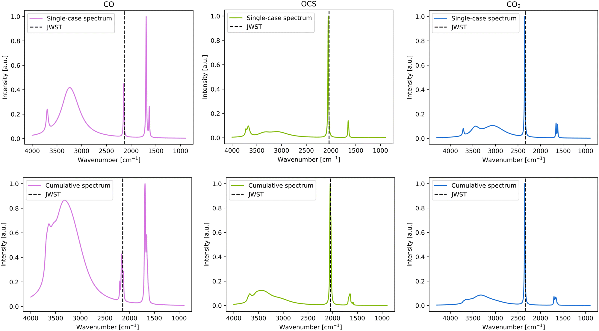Fig. 5 Left panels: Simulated IR spectra for CO corresponding to the most stable case (top) and to the cumulative plot (bottom), including the detected signal by JWST (dotted line). Central panels: Simulated IR spectra for OCS corresponding to the most stable case (top) and to the cumulative plot (bottom), including the detected signal by JWST (dotted lines). Right panels: Simulated IR spectra for CO₂ corresponding to the most stable case (top) and to the cumulative plot (bottom), including the detected signal by JWST (dotted line). The frequency unit is cm⁻¹, while the intensity is in arbitrary unit.

For CO, the single-case simulated adsorption presents the frequency at 2149 cm⁻¹, which is in good agreement with the JWST observations and the experimental measurements (2140 cm⁻¹ and 2139 cm⁻¹, respectively, see Table 3 and Fig. 5). In the cumulative plot, the band is somewhat broadened and ranges from 2120–2200 cm⁻¹, still it is consistent with the JWST observations (see Fig. 5). Such a broadening is caused by the different strength interactions (represented by the different BE values, and hence different perturbations) for each CO position on the surface, influencing the values of the individual peak positions, which are reflected in the cumulative plot.

For the CO₂ case, there is little to no difference in the C–O stretching peak between the single-case and the cumulative plots (see Fig. 5), which is indicative that this peak is almost unperturbed due to interaction with the water ice surface because adsorption results with similar frequency values in any of the binding sites. Comparison with the JWST spectra is fair (the computed value being 10 cm⁻¹ higher than the observational one), while comparison with experiments reveals that the computed frequency is overestimated by 20 cm⁻¹ with respect to the CO₂/ice cold mixture.

For OCS, the C–O stretching frequency is the lowest of all-detected bands of the considered species, at 2040 cm⁻¹. Like in the case of CO₂, neither in the single-case nor in the cumulative spectra, the band is broad, also indicating that this frequency is not affected whether adsorbed on one site or another. Moreover, both species have similar BE ranges, which can be considered broad (see Section 3.1), which is inversely proportional with the broadening of the IR peak. The computed frequencies of OCS are highly consistent with the experimental adsorbate/water ice mixture (a discrepancy of only 3 cm⁻¹), while it is overestimated by 11 cm⁻¹ with respect to the JWST one (see Table 3).

3.3.3 CH₄. For CH₄, the most weakly bound species to the amorphous water ice surface, its characteristic peaks (CH₄ bending and stretching modes) are visible in both simulated plots (see Fig. 6), which is particularly important for the stretching mode, as observationally it is overlapped by the broad O–H stretching mode of the dominant water ice components (especially the J110621 recorded spectrum⁶).

Fig. 6 Simulated IR spectra for CH₄ corresponding to the most stable case (top) and to the cumulative plot (bottom), including the detected signal by JWST (dotted lines). Frequency unit is cm⁻¹, while the intensity is in arbitrary unit.

Both peaks are slightly broadened in the cumulative spectra, and the computed frequencies are in very good agreement with the JWST observed and experimental values, particularly for the stretching mode, which exhibits discrepancies as small as 0.5 and 3.5 cm⁻¹, respectively (see Table 3).

4 Conclusions

This work provides a set of calculated binding energies, BE(0)s, for the most abundant molecules present in the interstellar ices besides H₂O (i.e., CO, CO₂, NH₃, CH₄, OCS and CH₃OH), which have been computed with the DFT B3LYP-D3(BJ) functional method on a periodic model surface mimicking an amorphous water ice. The new BE(0)s have been compared with earlier results,²² and used to assess the relative stability among the adsorption complexes. Moreover, IR spectral features of all the selected species on the water ice model have been computed and compared with the JWST results and with the experimental spectra recorded at very low T for adsorbate/ice mixtures.

Species considered in this work have been classified based on their H-bonding features with the ice as species that can act as H-bond donor and acceptors (Hb-DA: NH₃ and CH₃OH, with BE(0) > 3500 K), as H-bond acceptors (Hb-A: CO, CO₂ and OCS, with 3500 K > BE(0) > 1500 K), and not forming H-bonds (no-Hb: CH₄, with BE(0) < 1500 K), which interact with the surface mainly through dispersion forces. The comparison of the BE(0)s obtained in this work shows good agreement between previous computational works, as small discrepancies have been rationalized based on the better level of quantum chemical theory adopted here, B3LYP-D3(BJ), with respect to the one adopted in the previous work (DFT//HF-3c). It leads to a conclusion that the employed methodologies give an accurate description of the adsorption complexes and corresponding BE(0)s.

The effect of the adsorption of the species on the ice on their IR spectral features is shown. We included for all the cases the frequencies that come from the ice grain together with those specific to the adsorbates. In this way, we accounted for two aspects: (i) a direct comparability with both terrestrial lab adsorbate/ice mixture spectra, and (ii) the JWST spectra recorded for the real interstellar grains. Furthermore, we also discussed the role of the broad modes of ice as a plausible reason obscuring the components of the spectrum due to the overlap with the adsorbate vibrations. For that purpose, the most stable adsorption cases have been used to portrait the IR spectral features of each species as simulated spectra plots, along with a cumulative plot inclusive of the contributions coming from all the cases for each species. The comparison of the simulated spectral features with the experimental ice shows fair agreement for most cases. The best agreement is for CH₄ due to the very weak perturbation suffered by the vibrational frequency caused by the weak BE. For methanol, the OH stretching frequency value suffers from the lack of anharmonicity, which may easily move the frequency toward lower values, by about 100 cm⁻¹.⁶⁹ Simulated spectra are consistent with the absorption bands detected by the JWST as well as with the experimental ice spectra found in astrochemical databases. Moreover, when looking at our modelled frequencies for the adsorbed species, we are generally underestimating the shift suffered by the frequency of the adsorbates compared to both JWST and the laboratory mixture ice cold experiments. We suggest this as due to the nature of our model, in which the adsorption occurs only at the ice surface. In the real systems, the adsorbate can be embedded entirely in the ice matrix, a fact which may perturb the adsorbate vibrational modes more deeply than when adsorbed at the ice surface. Future work by our group will explore the role of the ice matrix on the fine aspects of the infrared spectra.

With this work, we show that quantum chemical simulations can be a useful tool for spectral analysis of IR signatures of the interstellar icy species. In some instances, it can provide more details about the observed spectral lines than experimental data and could be considered as another aid for the resolving the spectra and identification of the overlapped spectral lines.

Data availability

The data supporting this article have been included as part of the ESI.† Structures of the atomistic models are available at https://zenodo.org/records/15017748.

Conflicts of interest

There are no conflicts to declare.

Acknowledgements

This project has received funding from the European Union's Horizon 2020 research and innovation program from the European Research Council (ERC) for the project “Quantum Chemistry on Interstellar Grains” (QUANTUMGRAIN), grant agreement no 865657. MICIN (projects PID2021-126427NB-I00 and CNS2023-144902) is also acknowledged. The Italian Space Agency for co-funding the Life in Space Project (ASI N. 2019-3-U.O), the Italian MUR (PRIN 2020, Astrochemistry beyond the second period elements, Prot. 2020AFB3FX) are also acknowledged for financial support. Support from the Project CH4.0 under the MUR program “Dipartimenti di Eccellenza 2023-2027” (CUP: D13C22003520001) is also acknowledged. The authors thankfully acknowledge the supercomputational facilities provided by CSUC. A. R. gratefully acknowledges support through 2023 ICREA Award.

References

1. E. A. Bergin, G. A. Blake, F. Ciesla, M. M. Hirschmann and J. Li, Proc. Natl. Acad. Sci. U. S. A., 2015, 112, 8965–8970.
2. K. M. Ferrière, Rev. Mod. Phys., 2001, 73, 1031–1066.
3. T. Henning, Annu. Rev. Astron. Astrophys., 2010, 48, 21–46.
4. A. G. G. M. Tielens, Annu. Rev. Astron. Astrophys., 2008, 46, 289–337.
5. A. A. Boogert, P. A. Gerakines and D. C. Whittet, Annu. Rev. Astron. Astrophys., 2015, 53, 541–581.
6. M. K. McClure, W. R. M. Rocha, K. M. Pontoppidan, N. Crouzet, L. E. U. Chu, E. Dartois, T. Lamberts, J. A. Noble, Y. J. Pendleton, G. Perotti, D. Qasim, M. G. Rachid, Z. L. Smith, F. Sun, T. L. Beck, A. C. A. Boogert, W. A. Brown, P. Caselli, S. B. Charnley, H. M. Cuppen, H. Dickinson, M. N. Drozdovskaya, E. Egami, J. Erkal, H. Fraser, R. T. Garrod, D. Harsono, S. Ioppolo, I. Jiménez-Serra, M. Jin, J. K. Jørgensen, L. E. Kristensen, D. C. Lis, M. R. S. McCoustra, B. A. McGuire, G. J. Melnick, K. I. Öberg, M. E. Palumbo, T. Shimonishi, J. A. Sturm, E. F. van Dishoeck and H. Linnartz, Nat. Astron., 2023, 431–443.
7. A. McKellar, Publ. Astron. Soc. Pac., 1940, 52, 187.
8. A. E. Douglas and G. Herzberg, Can. J. Res., 1942, 20a, 71–82.
9. H. C. van de Hulst, Rech. Astron. Obs. Utrecht, 1946, 11, 2.i-2.
10. F. C. Gillett and W. J. Forrest, Astrophys. J., 1973, 179, 483.
11. S. Yamamoto, Introduction to astrochemistry, Springer, Tokyo, Japan, 1st edn, 2017.
12. A. Leger, S. Gauthier, D. Defourneau and D. Rouan, Astron. Astrophys., 1983, 117, 164–169.
13. S. I. H. Linnartz and G. Fedoseev, Int. Rev. Phys. Chem., 2015, 34, 205–237.
14. L. J. Allamandola, M. P. Bernstein, S. A. Sandford and R. L. Walker, Composition and Origin of Cometary Materials, Springer Netherlands, Dordrecht, 1999, pp. 219–232.
15. C. Ceccarelli, Faraday Discuss., 2023, 245, 11–51.
16. J. A. Noble, P. Theule, F. Mispelaer, F. Duvernay, G. Danger, E. Congiu, F. Dulieu and T. Chiavassa, Astron. Astrophys., 2012, 543, A5.
17. F. Dulieu, E. Congiu, J. Noble, S. Baouche, H. Chaabouni, A. Moudens, M. Minissale and S. Cazaux, Sci. Rep., 2013, 3, 1338.
18. J. He, K. Acharyya and G. Vidali, Astrophys. J., 2016, 825, 89.
19. H. Chaabouni, S. Diana, T. Nguyen and F. Dulieu, Astron. Astrophys., 2018, 612, A47.
20. M. Minissale, Y. Aikawa, E. Bergin, M. Bertin, W. A. Brown, S. Cazaux, S. B. Charnley, A. Coutens, H. M. Cuppen, V. Guzman, H. Linnartz, M. R. McCoustra, A. Rimola, J. G. Schrauwen, C. Toubin, P. Ugliengo, N. Watanabe, V. Wakelam and F. Dulieu, ACS Earth Space Chem., 2022, 6, 597–630.
21. V. Wakelam, J. C. Loison, R. Mereau and M. Ruaud, Mol. Astrophys., 2017, 6, 22–35.
22. S. Ferrero, L. Zamirri, C. Ceccarelli, A. Witzel, A. Rimola and P. Ugliengo, Astrophys. J., 2020, 904, 11.
23. J. Perrero, J. Enrique-Romero, S. Ferrero, C. Ceccarelli, L. Podio, C. Codella, A. Rimola and P. Ugliengo, Astrophys. J., 2022, 938, 158.
24. G. M. Bovolenta, S. Vogt-Geisse, S. Bovino and T. Grassi, Astrophys. J., Suppl. Ser., 2022, 262, 17.
25. B. Martínez-Bachs, S. Ferrero, C. Ceccarelli, P. Ugliengo and A. Rimola, Astrophys. J., 2024, 969, 63.
26. V. Bariosco, S. Pantaleone, C. Ceccarelli, A. Rimola, N. Balucani, M. Corno and P. Ugliengo, Mon. Not. R. Astron. Soc., 2024, 531, 1371–1384.
27. Z. Dohnálek, G. A. Kimmel, S. A. Joyce, P. Ayotte, R. S. Smith and B. D. Kay, J. Phys. Chem. B, 2001, 105, 3747–3751.
28. B. A. McGuire, Astrophys. J., Suppl. Ser., 2022, 259, 30.
29. E. Herbst and E. F. van Dishoeck, Ann. Rev. Astron. Astrophys., 2009, 47, 427–480.
30. C. Ceccarelli, P. Caselli, F. Fontani, R. Neri, A. López-Sepulcre, C. Codella, S. Feng, I. Jiménez-Serra, B. Lefloch, J. E. Pineda, C. Vastel, F. Alves, R. Bachiller, N. Balucani, E. Bianchi, L. Bizzocchi, S. Bottinelli, E. Caux, A. Chacón-Tanarro, R. Choudhury, A. Coutens, F. Dulieu, C. Favre, P. Hily-Blant, J. Holdship, C. Kahane, A. Jaber Al-Edhari, J. Laas, J. Ospina, Y. Oya, L. Podio, A. Pon, A. Punanova, D. Quenard, A. Rimola, N. Sakai, I. R. Sims, S. Spezzano, V. Taquet, L. Testi, P. Theulé, P. Ugliengo, A. I. Vasyunin, S. Viti, L. Wiesenfeld and S. Yamamoto, Astrophys. J., 2017, 850, 176.
31. J. P. Gardner, J. C. Mather, R. Abbott, J. S. Abell, M. Abernathy, F. E. Abney, J. G. Abraham, R. Abraham, Y. M. Abul-Huda, S. Acton and C. K. Adams, Publ. Astron. Soc. Pac., 2023, 135, 068001.
32. K. I. Öberg, A. C. Boogert, K. M. Pontoppidan, S. V. D. Broek, E. F. V. Dishoeck, S. Bottinelli, G. A. Blake and N. J. Evans, Astrophys. J., 2011, 740, 109.
33. J. A. Sturm, M. K. McClure, T. L. Beck, D. Harsono, J. B. Bergner, E. Dartois, A. C. Boogert, J. E. Chiar, M. A. Cordiner, M. N. Drozdovskaya, S. Ioppolo, C. J. Law, H. Linnartz, D. C. Lis, G. J. Melnick, B. A. McGuire, J. A. Noble, K. I. Oberg, M. E. Palumbo, Y. J. Pendleton, G. Perotti, K. M. Pontoppidan, D. Qasim, W. R. Rocha, H. Terada, R. G. Urso and E. F. V. Dishoeck, Astron. Astrophys., 2023, 679, A138.
34. K. I. Öberg, Chem. Rev., 2016, 116, 9631–9663.
35. W. R. Rocha, E. F. V. Dishoeck, M. E. Ressler, M. L. V. Gelder, K. Slavicinska, N. G. Brunken, H. Linnartz, T. P. Ray, H. Beuther, A. C. O. Garatti, V. Geers, P. J. Kavanagh, P. D. Klaassen, K. Justtanont, Y. Chen, L. Francis, C. Gieser, G. Perotti, Ł. Tychoniec, M. Barsony, L. Majumdar, V. J. L. Gouellec, L. E. Chu, B. W. Lew, T. Henning and G. Wright, Astron. Astrophys., 2024, 683, A124.
36. H. Linnartz, J. B. Bossa, J. Bouwman, H. M. Cuppen, S. H. Cuylle, E. F. V. Dishoeck, E. C. Fayolle, G. Fedoseev, G. W. Fuchs, S. Ioppolo, K. Isokoski, T. Lamberts, K. I. Oberg, C. Romanzin, E. Tenenbaum and J. Zhen, Proc. Int. Astron. Union, 2011, 7, 390–404.
37. W. R. Rocha, M. G. Rachid, B. Olsthoorn, E. F. V. Dishoeck, M. K. McClure and H. Linnartz, Astron. Astrophys., 2022, 668, A63.
38. HEJDOC, Heidelberg-Jena-Database of Optical Constants, https://www2.mpia-hd.mpg.de/HJPDOC/content.php, 2025.
39. R. C. Fortenberry, Int. J. Quantum Chem., 2017, 117, 81–91.
40. R. Sure and S. Grimme, J. Comput. Chem., 2013, 34, 1672–1685.
41. W. Hagen, A. G. G. Tielens and J. M. Greenberg, Chem. Phys., 1981, 56, 367–379.
42. T. Shimonishi, N. Nakatani, K. Furuya and T. Hama, Astrophys. J., 2018, 855, 27.
43. R. Dovesi, A. Erba, R. Orlando, C. M. Zicovich-Wilson, B. Civalleri, L. Maschio, M. Rérat, S. Casassa, J. Baima, S. Salustro and B. Kirtman, Wiley Interdiscip. Rev.: Comput. Mol. Sci., 2018, 8, e1360.
44. C. Lee, W. Yang and R. G. Parr, Phys. Rev. B: Condens. Matter Mater. Phys., 1988, 37, 785–789.
45. A. D. Becke, J. Chem. Phys., 1993, 98, 1372–1377.
46. S. Grimme, J. Antony, S. Ehrlich and H. Krieg, J. Chem. Phys., 2010, 132, 154104.
47. S. Grimme, S. Ehrlich and L. Goerigk, J. Comput. Chem., 2011, 32, 1456–1465.
48. S. Grimme, A. Hansen, J. G. Brandenburg and C. Bannwarth, Chem. Rev., 2016, 116, 5105–5154.
49. A. Schäfer, H. Horn and R. Ahlrichs, J. Chem. Phys., 1992, 97, 2571–2577.
50. A. Germain, L. Tinacci, S. Pantaleone, C. Ceccarelli and P. Ugliengo, ACS Earth Space Chem., 2022, 6, 1286–1298.
51. L. Tinacci, A. Germain, S. Pantaleone, C. Ceccarelli, N. Balucani and P. Ugliengo, Astrophys. J., 2023, 951, 32.
52. E. Mates-Torres and A. Rimola, J. Appl. Crystallogr., 2024, 57, 503–508.
53. V. Bariosco, L. Tinacci, S. Pantaleone, C. Ceccarelli, A. Rimola and P. Ugliengo, Mon. Not. R. Astron. Soc., 2025, 539, 82–94.
54. F. Pascale, C. M. Zicovich-Wilson, F. López Gejo, B. Civalleri, R. Orlando and R. Dovesi, J. Comput. Chem., 2004, 25, 888–897.
55. C. M. Zicovich-Wilson, F. Pascale, C. Roetti, V. R. Saunders, R. Orlando and R. Dovesi, J. Comput. Chem., 2004, 25, 1873–1881.
56. M. Ferrero, M. Rérat, R. Orlando and R. Dovesi, J. Chem. Phys., 2008, 128, 014110.
57. S. Boys and F. Bernardi, Mol. Phys., 1970, 19, 553–566.
58. E. R. Davidson and D. Feller, Chem. Rev., 1986, 86, 681–696.
59. R. D. Johnson, NIST Computational Chemistry Comparison and Benchmark Database NIST Standard Reference Database Number 101, 2022.
60. B. M. C. Huggins, G. C. Pimentel, R. C. Lord, B. Nolin and H. D. Stidham, J. Am. Chem. Soc., 1956, 6, 265–266.
61. N. Bancone, R. Santalucia, S. Pantaleone, P. Ugliengo, L. Mino, A. Rimola and M. Corno, J. Phys. Chem. C, 2024, 128, 15171–15178.
62. J. Perrero, P. Ugliengo, C. Ceccarelli and A. Rimola, Mon. Not. R. Astron. Soc., 2023, 525, 2654–2667.
63. M. Moore, R. Ferrante, R. Hudson and J. Stone, Icarus, 2007, 190, 260–273.
64. W. Hagen, A. G. G. M. Tielens and J. M. Greenberg, Astron. Astrophys., Suppl. Ser., 1983, 51, 389–416.
65. M. Palumbo, A. G. G. M. Tielens and A. T. Tokunaga, Astrophys. J., 1995, 449, 674–680.
66. G. Mulas, G. A. Baratta, M. E. Palumbo and G. Strazzulla, Profile of CH 4 IR bands in ice mixtures, 1998.
67. A. C. A. Boogert, K. Brewer, A. Brittain and K. S. Emerson, Astrophys. J., 2022, 941, 32.
68. L. Zamirri, S. Casassa, A. Rimola, M. Segado-Centellas, C. Ceccarelli and P. Ugliengo, Mon. Not. R. Astron. Soc., 2018, 480, 1427–1444.
69. P. Ugliengo, F. Pascale, M. Mérawa, P. Labéguerie, S. Tosoni and R. Dovesi, J. Phys. Chem. B, 2004, 108, 13632–13637.

---

Footnote

† Electronic supplementary information (ESI) available. See DOI: https://doi.org/10.1039/d5cp01151e

---