
 Open Access Article
 This Open Access Article is licensed under a Creative Commons Attribution-Non Commercial 3.0 Unported Licence
Incoherent tunneling surface diffusion
E. E.
Torres-Miyares
 *ab and
S.
Miret-Artés
b
*ab and
S.
Miret-Artés
b
aFundación Humanismo y Ciencia, Guzmán el Bueno 66, 28015 Madrid, Spain. E-mail: elena.torres@iff.csic.es
bInstituto de Física Fundamental, Consejo Superior de Investigaciones Científicas, Serrano 123, 28006 Madrid, Spain. E-mail: s.miret@iff.csic.es
First published on 26th June 2025
Abstract
In this work, incoherent tunneling surface diffusion is analyzed by means of the stochastic wave function (SWF) method within the Lindblad formalism. Previous calculations based on the transition state theory (TST) were unable to provide reasonable values of friction coefficients for the diffusion motion of H and D adsorbates on a Pt(111) surface. Thermal activation and tunneling regimes were covered by varying the surface temperature, approaching the so-called cross-over temperature. Numerical results for the total hopping/tunneling rates are fairly good when compared to the experimental values by assuming a simple cosine corrugation function. No fitting has been carried out and estimated values of the physical parameters (friction coefficients, well and barrier frequencies and barrier height), extracted from the thermal activation regime, are used. Finally, survival probabilities on the different wells are also reported.
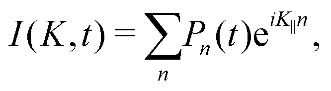
Incoherent tunneling surface diffussion is a theoretical challenge. In 2010, the Cambridge group analyzed the diffusion motion of H and D adsorbates on a Pt(111) surface by means of the spin-echo He (HeSE) scattering experimental technique.1 In the so-called diffusive time regime (when time is much greater than the inverse of the friction), it is generally assumed that the so-called intermediate scattering function (ISF) can be fitted by an exponential function of time according to
| I(K, t) = Be−α(K)t + C, | (1) |
The corresponding measurements indicated that quantum effects are significant at low temperatures. The range of temperatures used went from 250 K up to 80 K, covering thermal activation and tunneling regimes. The crossover temperature was estimated to be 66 K for H and 63 K for D. Furthermore, the diffusion motion seems to correspond to nearest neighbor hopping for a coverage of 0.1 ML, along the [11![[2 with combining macron]](https://www.rsc.org/images/entities/char_0032_0304.gif) ] direction. Following this CE model, deviations from nearest neighbor random jumps for H and D between fcc hollow sites were reported to be minimal. Diffusion dynamics was also claimed to take place in the moderate-to-high friction regime. The quantum TST of dissipative tunneling for temperatures above the crossover covering tunneling and thermal activation should be applied. From this theory and by assuming a parabolic barrier, one should easily extract information on the corresponding physical parameters. Finally, despite a very good fitting to the experimental jumping/tunneling rates versus the inverse of the surface temperature, the friction values reported were unreasonable large (of the order of 1000 ps−1) and, therefore, the energy barrier can not be the same to the one we have used here. Another attempt to obtain friction values was based on path integrals for a periodic potential.3 The values reported were too small (of the order of a few ps−1) but no information on barriers and frequencies was provided.4 In both cases, the authors obtained very good fittings but with big numerical discrepancies, showing that good fittings are not enough.
] direction. Following this CE model, deviations from nearest neighbor random jumps for H and D between fcc hollow sites were reported to be minimal. Diffusion dynamics was also claimed to take place in the moderate-to-high friction regime. The quantum TST of dissipative tunneling for temperatures above the crossover covering tunneling and thermal activation should be applied. From this theory and by assuming a parabolic barrier, one should easily extract information on the corresponding physical parameters. Finally, despite a very good fitting to the experimental jumping/tunneling rates versus the inverse of the surface temperature, the friction values reported were unreasonable large (of the order of 1000 ps−1) and, therefore, the energy barrier can not be the same to the one we have used here. Another attempt to obtain friction values was based on path integrals for a periodic potential.3 The values reported were too small (of the order of a few ps−1) but no information on barriers and frequencies was provided.4 In both cases, the authors obtained very good fittings but with big numerical discrepancies, showing that good fittings are not enough.
The tunneling rates were calculated from closed expressions using Kramers' theory.5 It is generally assumed that tunneling proceeds via a parabolic barrier.6 Within the extended TST, the tunneling rate can be expressed as
 | (2) |
 defined in ref. 1. The factor N is an integer describing the number of equal directions for escape from a given well and is determined by the direction of observation and the geometry of the surface. For a triangular surface structure as the Pt(111), there are three equal directions for escape. However, for the [11] direction, N = 2 and not N = 3 as used in ref. 1 since one surface site is dark along that direction.9 The Wolynes factor Ξ is the parabolic barrier based ratio of the quantum partition function at the barrier to that of the well6
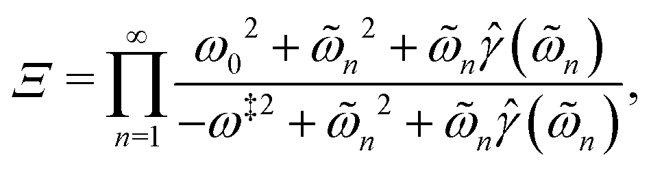 | (3) |
![[small omega, Greek, tilde]](https://www.rsc.org/images/entities/i_char_e10f.gif) n = 2πn/ħβ, and
n = 2πn/ħβ, and ![[small gamma, Greek, circumflex]](https://www.rsc.org/images/entities/i_char_e0b2.gif) (s), the Laplace transform of the time dependent friction. In the classical limit, all the Matsubara frequencies go to infinity and Ξ → 1 and one recovers the classical Kramers' limit for the rate. This fact could be used to extract, in this case, some good estimates of the physical parameters mentioned above. In the classical limit, the Wolynes factor plays a minor role and therefore one could extract an estimated value for the barrier height from two surface temperatures in the linear region of the experimental Arrhenius plot according to eqn (2). Thus, this value is V‡ = 72 meV for H and D versus to 83 meV.1 By assuming a parabolic barrier, we have chosen ħω0 = ħω‡ = 30 meV, where this value is issued from HREELS measurements10 for H (the corresponding frequency for D is given by
(s), the Laplace transform of the time dependent friction. In the classical limit, all the Matsubara frequencies go to infinity and Ξ → 1 and one recovers the classical Kramers' limit for the rate. This fact could be used to extract, in this case, some good estimates of the physical parameters mentioned above. In the classical limit, the Wolynes factor plays a minor role and therefore one could extract an estimated value for the barrier height from two surface temperatures in the linear region of the experimental Arrhenius plot according to eqn (2). Thus, this value is V‡ = 72 meV for H and D versus to 83 meV.1 By assuming a parabolic barrier, we have chosen ħω0 = ħω‡ = 30 meV, where this value is issued from HREELS measurements10 for H (the corresponding frequency for D is given by 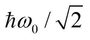 due to the relation between masses). Thus, only the friction coefficient is left (if Ohmic friction is also assumed). From the same equation, estimated values for friction are 140 ps−1 and 70 ps−1 for H and D, respectively; values which seem to be much more reasonable than those previously published1,4 and could explain, in a certain sense, why first neighbor sites are prominent in this diffusion.
Very often, parabolic barriers are not good enough and anharmonic effects are needed in order to extract reliable fitting physical parameters. Moreover, in the vicinity of the crossover temperature, some divergences are found in the theory; the Wolynes factor diverges at the crossover temperature defined as ħβcλ‡ = 2π, where βc = 1/kTc, k and Tc being the Boltzmann constant and the crossover temperature, respectively. This divergence has been recently removed using the uniform semiclassical energy-dependent transmission coefficient. The resulting one-dimensional theory11 has been generalized to dissipative systems12 and may be used to analyze the experimental data. The uniform Wolynes factor is clearly responsible for the change of slope around the crossover surface temperature. However, the bending of the straight line experienced by the tunneling rates around Tc is a real open problem. One of the critical problems in the standard and extended theory used comes from a fundamental assumption. In order to provide closed formulas, and considering Ohmic friction, one has to assume the separable motion between the so-called unstable normal mode and the stable modes along the reaction or symmetry coordinate; in other words, their coupling should be very weak. This assumption could not take place or be in the limit of applicability of the theory in ref. 1. This makes far from trivial the theoretical treatment in order to reach workable expressions for carrying out a fitting procedure. Therefore, in general, several problems should be stressed for this purpose. First, one is faced to fit at the same time at least 4 parameters (friction coefficient, barrier height, well and barrier frequencies and, sometimes, anharmonic corrections to a parabolic barrier). The dimensionality of the space of parameters is thus too high; the fitting procedure is carried out in a global way, not sequential. Second, the different conditions that the theory demands in order to be applicable to reach closed expressions have to be added as constraints; in particular, as mentioned before, if the motion between the stable and unstable modes can be assumed separable. And, third, even if the divergence of the Wolynes factor has been recently removed, it is not clear that a better theory is coming soon; several conditions and/or constraints have also to be fulfilled in the fitting process. In the meantime, one way to skip such difficulties is, in our opinion, the procedure we use in this work. Our starting point is thus different and based on the so-called SWF method.13–15
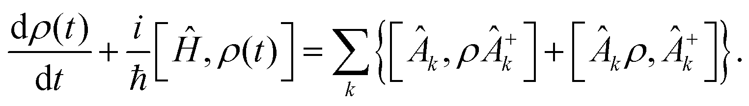
The ISF, I(K, t), is related to the probability density ρ(R, t) through a space Fourier transforms as follows13–15
 | (4) |
 | (5) |
A single Lindblad operator Âk is used, given by a linear combination of the position operator ![[x with combining circumflex]](https://www.rsc.org/images/entities/i_char_0078_0302.gif) and the momentum operator
and the momentum operator ![[p with combining circumflex]](https://www.rsc.org/images/entities/i_char_0070_0302.gif) . In the coordinate representation, this equation leads to an Î to stochastic differential equation which is solved for a high number of stochastic wave functions or realizations. The ISF can then be obtained through an average over stochastic realizations
. In the coordinate representation, this equation leads to an Î to stochastic differential equation which is solved for a high number of stochastic wave functions or realizations. The ISF can then be obtained through an average over stochastic realizations
| I(K, t) = 〈e−iK·(0)eiK·(t)〉. | (6) |
A potential with a single Fourier component is assumed: V(x) = V0![[thin space (1/6-em)]](https://www.rsc.org/images/entities/char_2009.gif) cos(2πx/a), with an energy barrier V‡ = 2V0 and a lattice length of a = 2.77 Å for the Pt(111) surface. The numerical code is parallelized and the number of realizations Nr = 100000 is chosen to reach the numerical stability for the mean value expressed in eqn (6). The numerical simulations are run up to 40 ps with a time step of 0.05 ps, by starting with an initial Gaussian wave packet centered at x = 0, with a width of 0.79 Å and momentum distributed according to the Maxwell–Boltzmann distribution
cos(2πx/a), with an energy barrier V‡ = 2V0 and a lattice length of a = 2.77 Å for the Pt(111) surface. The numerical code is parallelized and the number of realizations Nr = 100000 is chosen to reach the numerical stability for the mean value expressed in eqn (6). The numerical simulations are run up to 40 ps with a time step of 0.05 ps, by starting with an initial Gaussian wave packet centered at x = 0, with a width of 0.79 Å and momentum distributed according to the Maxwell–Boltzmann distribution  . A one-dimensional space within the interval [−4.2, 4.2] Å is used with Ns = 4096 points, resulting in a space step of Δx = 0.002 Å. At long times, t ≫ γ−1, the ISF is expected to decay as eqn (1) and this allows us to extract the dephasing rate for each value of K. The cut-off time for fitting the tail of the ISF to an exponential function of time is chosen to be 8.2 ps, following the same procedure as in the experimental case; that is, when a certain region of stability of the dephasing rate is observed, which has also to be of the order of the experimental rate value.
Within the CE jump model, if a simple Bravais lattice is assumed as well as instantaneous jumps between different sites, and only transitions between first neighbors are going to be allowed (the diffusion dynamics is assumed to be one-dimensional on a periodic substrate), a Pauli master equation can be written in terms of probabilities as4
| Ṗn(t) = Γ+n−1P(t)n−1 + Γ−n+1P(t)n+1 − (Γ+n + Γ−n)Pn(t), | (7) |
| Pn(t) = In(Γt)e−Γt, | (8) |
 | (9) |
![[thin space (1/6-em)]](https://www.rsc.org/images/entities/i_char_2009.gif) cos(β), β being the angle formed by the direction of observation and diffusion symmetry direction (in our case, β = π/6 for the two symmetry directions allowed by K). The ISF can also be recast as
cos(β), β being the angle formed by the direction of observation and diffusion symmetry direction (in our case, β = π/6 for the two symmetry directions allowed by K). The ISF can also be recast as | (10) |
 | (11) |
This analytical expression is quite different from the one used in ref. 4, as they arise from different theoretical frameworks.
In Fig. 1, Arrhenius-like plots of the temperature dependence of the tunneling/hopping rates issued from the experimental results1 for H (red circles) and D (red triangles) diffusion and momentum transfer of K = 0.86 Å−1 are plotted. Numerical simulations are also included coming from the SWF method (NS blue points). The experimental total hopping rates have been supposed to have three directions of diffusion but, according to the direction of observation chosen, only two are possible.9 Thus, these ones have been multiplied by a factor 2/3 in order to take into account that in this case N = 2. As can be seen, the agreement is fairly good for all surface temperatures; in particular, at low temperatures close to the cross-over one. The hopping rates for D are consistently smaller than those for H across the entire temperature range, indicating a clear mass effect. For H diffusion, if one assumes that the Arrhenius classical law is due to thermal activation only, one then could compare the corresponding hopping rate to the experimental/numerical one at different surface temperatures. Thus, for 214 K, hops by thermal activation dominate 100–90%; for 80 K, only hops by tunneling predominates, around 90%; and for 121 K, hops for thermal activation and tunneling are around 30% and 70%, respectively.
 | ||
| Fig. 1 Arrhenius-like plots of the temperature dependence of the tunneling rate issued from the experimental results shown in ref. 1 for H diffusion (red circles) and D (red triangles) diffusion at a momentum transfer of K= 0.86 Å−1. Numerical simulations (NS blue points) using a energy barrier of V = 72 meV and a friction coefficient of 140 ps−1 for H (blue square) and 70 ps−1 for D (blue star) are also plotted and issued from the SWF method (assuming the same friction, barrier height, and vibrational frequencies across all temperatures). | ||
Finally, another useful information which can be extracted from the experimental results for the total hopping/tunneling rates is the probability to stay in a given surface site (survival probability). This information has not been given so far in this context. From eqn (8), this probability as a function of time is easily calculated once the tunneling/hopping rates are known. In Fig. 2, the time dependence of the probability of staying at the zero, P0(t) (blue curve), first, P1(t) (black curve), and second, P2(t) (red curve), well are plotted for H adsorbates on a Pt(111) surface at three different temperatures, covering the classical and quantum regimes: 214 K, 121 K and 80 K. These calculations are carried out using the experimental tunneling rates shown in Fig. 1. As clearly seen in this figure, at 214 K and 121 K, P0(t) and P1(t) suddenly start with a maximum probability and decreasing with time very rapidly due to the thermal activation (classical regime). Pn(t) functions could also be seen as survival probabilities to remain in a given well. Obviously, P2(t) displays the same pattern but with a smaller maximum value. The third temperature displays a different time behavior since we are in the quantum regime. Here it is supposed that tunneling plays a major role and the sudden increase at very short times is not longer observed. Furthermore, the decreasing of P1(t) and P2(t) with time is not so rapid because the tunneling diffusion takes time since Γ is small. The asymptotic values observed for the survival probabilities indicate us that at a sufficiently long time these probabilities are nearly constant where thermal equilibrium is already reached. At these long times hopping/transition dynamics could repopulate surface sites such as 0, 1, 2, etc.
 | ||
| Fig. 2 Time dependence of the probability of staying (survival probabilities) at the initial well P0(t) (blue curve), the first P1(t) (black curve), and the second P2(t) (red curves) well from eqn (8) for H adsorbates on a Pt(111) surface is plotted at three different temperatures: 214 K, 121 K and 80 K. These calculations are carried out using the corresponding experimental hopping/tunneling rates obtained for a momentum transfer of K = 0.86 Å−1 along the [11] direction and a coverage of 0.1 ML. | ||
Along this work, we have focused on a theoretical challenge, the incoherent tunneling diffusion. The choice of H and D diffusion by a Pt(111) surface in order to illustrate this transition is by no means arbitrary. Unreasonable friction values were reported as well as the standard and extended TST for this case is now questionable. The SWF method within the Lindblad formalism is able to provide reasonable results for the tunneling/hopping rates as a function of the inverse of surface temperature by assuming a simple cosine corrugation function. Physical parameters for friction, well and barrier frequencies as well as barrier height are estimated from the diffusion dynamics at high surface temperatures. Clearly, this numerical method is not convenient at all for a fitting procedure but, waiting for a better analytical theory within the TST formalism, it has shown to be a very good alternative, apart from being an exact theory within the Markovian approach. Obviously, ab initio calculations need to be done for a better description of this tunneling diffusion. ref. 16 should be a good starting point. For other systems, with a different adsorbate or surface symmetry, may require going beyond a 1D model, and the hopping rates cannot be captured by a simple scaling factor. Furthermore, it is also very illustrative to show survival probabilities for different wells which decay exponentially with time, exp(−Γt).
Author contributions
All authors have contributed equally to this work.Conflicts of interest
There are no conflicts to declare.Data availability
All data supporting the findings of this study are included within the article.Acknowledgements
E. E. T.-M. would like to thank Fundación Humanismo y Ciencia for financial support. E. E. T.-M. and S. M.-A. acknowledge support of a grant from the Ministry of Science, Innovation and Universities with Ref. PID2023-149406NB-I00. Prof. Eli Pollak is acknowledged for very useful and illuminating discussions in this open problem. We would like to thank an anonymous referee for very helpful comments.References
- A. Jardine, E. Lee, D. Ward, G. Alexandrowicz, H. Hedgeland, W. Allison, J. Ellis and E. Pollak, Phys. Rev. Lett., 2010, 105, 136101 CrossRef CAS PubMed.
- C. T. Chudley and R. J. Elliott, Proc. Phys. Soc., 1961, 77, 353 CrossRef.
- U. Weiss and H. Grabert, Phys. Lett. A, 1985, 108, 63–67 CrossRef.
- A. Sanz, R. Martínez-Casado and S. Miret-Artés, Surf. Sci., 2013, 617, 229–232 CrossRef CAS.
- E. Pollak and S. Miret-Artés, Chem. Phys. Chem., 2023, 24, e202300272 CrossRef CAS PubMed.
- P. G. Wolynes, Phys. Rev. Lett., 1981, 47, 968 CrossRef CAS.
- H. A. Kramers, Physica, 1940, 7, 284–304 CrossRef CAS.
- R. F. Grote and J. T. Hynes, J. Chem. Phys., 1980, 73, 2715–2732 CrossRef CAS.
- A. Graham, A. Menzel and J. Toennies, J. Chem. Phys., 1999, 111, 1676–1685 CrossRef CAS.
- S. Bădesu, P. Salo, T. Ala-Nissila, S. Ying, K. Jacobi, Y. Wang, K. Bedürftig and G. Ertl, Phys. Rev. Lett., 2002, 88, 136101 CrossRef PubMed.
- S. Upadhyayula and E. Pollak, J. Phys. Chem. Lett., 2023, 14, 9892–9899 CrossRef CAS PubMed.
- E. Pollak, Phys. Rev. A, 2024, 109, 022242 CrossRef CAS.
- E. E. Torres-Miyares, G. Rojas-Lorenzo, J. Rubayo-Soneira and S. Miret-Artés, Mathematics, 2021, 9, 362 CrossRef.
- E. E. Torres-Miyares, G. Rojas-Lorenzo, J. Rubayo-Soneira and S. Miret-Artés, Phys. Chem. Chem. Phys., 2022, 24, 15871–15890 RSC.
- E. E. Torres-Miyares, D. Ward, G. Rojas-Lorenzo, J. Rubayo-Soneira, W. Allison and S. Miret-Artés, Phys. Chem. Chem. Phys., 2023, 25, 6225–6231 RSC.
- C. Bi and Y. Yang, J. Phys. Chem. C, 2021, 125, 464–480 CrossRef CAS.
| This journal is © the Owner Societies 2025 |