
 Open Access Article
 This Open Access Article is licensed under a
 Creative Commons Attribution 3.0 Unported Licence
Relaxation dynamics of aniline in methanol: the photoionization channel†
Raúl
Montero
 ab,
Iker
Lamas
a,
Marta
Fernández-Fernández
a,
Andrew W.
Prentice
c,
Dave
Townsend
cd,
Martin J.
Paterson
c and
Asier
Longarte
*a
ab,
Iker
Lamas
a,
Marta
Fernández-Fernández
a,
Andrew W.
Prentice
c,
Dave
Townsend
cd,
Martin J.
Paterson
c and
Asier
Longarte
*a
aDepartamento de Química Física, Universidad del País Vasco (UPV/EHU), Apart. 644, 48080 Bilbao, Spain. E-mail: asier.longarte@ehu.eus
bSGIker Laser Facility, Universidad del País Vasco (UPV/EHU), Leioa, Spain
cInstitute of Chemical Sciences, Heriot-Watt University, Edinburgh EH14 4AS, UK
dInstitute of Photonics & Quantum Sciences, Heriot-Watt University, Edinburgh EH14 4AS, UK
First published on 3rd July 2025
Abstract
The relaxation of aniline after excitation at 267 and 200 nm (4.6 and 6.2 eV) in methanol solutions has been explored by fs time-resolved experiments and the observations interpreted using ab initio calculations on the excited states of aniline–methanol clusters. In contrast to what has been reported under aqueous solvation, excitation at 267 nm does not induce ionization of the molecule and only a photophysical relaxation route is operative. The computational results allow us to rationalize this observation in terms of the different nature that the Rydberg transition, responsible for the electron ejection, presents in analogous N–H⋯O structures seen in methanol and water clusters. On the other hand, ionization of aniline via the direct ejection of an electron into the solvent is identified in methanol following 200 nm excitation, a mechanism analogous to that found in water at this energy.
Introduction
The processes triggered by the excitation of aromatic molecules substituted by amino groups in the ultraviolet (UV) and visible range have a vast importance in chemistry. In particular, they are valuable models to understand the photochemistry of more complex, closely related molecules with vital biological functions such as the adenine or guanine nucleobases.1–3 Accordingly, the photochemical and photophysical properties of aniline, the most simple and prototypical compound among the aromatic amines, has attracted the interest of chemists since early times.4,5The solvated aniline molecule exhibits an intricate behavior when its lowest electronic absorption band is photoexcited, which extends from 310 to 260 nm (4.0 to 4.8 eV) and corresponds to a ππ* transition from the ground to the S1 state (also labeled as Lb in Platt's nomenclature).6–8 Depending on the solvent and the specific excitation wavelength, a lifetime from 0.93 to 4.34 ns has been measured for this state.9 In addition to fluorescence, the relaxation is known to occur through a combination of intersystem crossing (ISC) and internal conversion (IC). While the former dominates in polar solvents giving rise to long-lived triplet states, the latter is the preferred channel in water.10 In parallel to this photophysical route, however, additional deactivation channels, which mainly involve the appearance of solvated electrons (1) and anilino radicals (2) have been described in aqueous4,10–12 and non-polar media,4,10,13 respectively.
| Ph-NH2 → Ph-NH2+ + e− | (1) |
| Ph-NH2 → Ph-NH˙ + H˙ | (2) |
The aniline behavior can be framed more generally in terms of the single-photon UV excitation and subsequent photoionization of aromatic molecules near the onset of their electronic absorptions – something discovered in aqueous media long ago.14,15 Considering the importance of reactions that generate charged species under solvated conditions at relatively low excitation energies, numerous works have targeted the characterization of this relaxation channel, specially, for tryptophane and indole derivatives.16–23 More recently, the photoionization mechanism of simple chromophores, as indole24–26 and phenol,27,28 has been investigated directly in water solutions using time-resolved methods based on fs laser pulses. The interpretation of the collected observations has been guided by the detailed knowledge provided by calculations about the influence of the solvent on electronic structure of the isolated molecules, in the micro-solvation environment of molecular clusters,29–31 and also directly in the aqueous medium.32,33
Focusing back on the aniline case, its photoionization in aqueous medium has been described at excitation energies as low as 308 nm (4.0 eV) in experiments with nanosecond laser pulse durations. At this level of temporal resolution, the formation of the cation and the solvated electron is observed to occur synchronously to the appearance of the S1 excited state, with a yield of ∼0.18.10 Recent experiments conducted on the fs time-scale when exciting aniline in water at 267 nm have allowed us to identify, within the experimental cross-correlation (CC) time, the formation of a charge transfer (CT) character state, together with the characteristic S1 ππ* excitation.34 Mainly grounded on the predictions of calculations for similar chromophores with O–H and N–H bonds interacting with water molecules,29–32,35–37 we proposed that this CT state would be the dark π3s/σ* excitation that has been identified in the relaxation dynamics of the isolated molecule.38–40 This state would be populated at short times, below the resolution of the experiment, from the prepared S1 ππ*. While the latter is responsible for the photophysical relaxation pathway, the former leads to the autoionization of the molecule, yielding fully solvated electrons and cations with a 0.5 ns lifetime. On the other hand, the presence of the aniline radical was not detected in the temporal observation window of the experiment (2 ns). Although deprotonation of the aniline radical cation should occur (according to the pKa = 6–7), this process (3) may take place on longer time-scales (μs).24
| Ph-NH2+ → Ph-NH˙ + H+ | (3) |
Building on the knowledge gained by these recent studies of the excited state dynamics of aqueous aniline,34 herein we present femtosecond (fs) time-resolved data obtained in the polar protic environment of methanol, covering the interval from the very early times after photoexcitation to the nanosecond domain. The ability of this solvent to hold solvated electrons is well known.41,42 Additionally, the methanol molecule is able to establish the same type of H-bond interactions with the amino group43,44 as those supported in water. This can promote the formation of the πσ* CT state that has been proposed to mediate the ionization of the molecule at low excitation energies in water.34 Contrary to the water case, however, the recorded measurements do not show any sign of the formation of this state. Furthermore, the appearance of electrons in the medium is not detected for excitation energies up to ∼6.2 eV (∼200 nm), well above the onset of the electronic absorption and the value (4.0 eV)10 measured in water. In order to rationalize the observed behavior, and in particular, the remarkable differences when compared to the aqueous medium, the electronic structure of An(Meth)1 has been calculated by ab initio methods. From the theoretically guided interpretation of the experimental observations, we obtain a detailed picture of the relaxation dynamics of this simple chromophore in solution, particularly regarding the ionization channel.
Experimental and computational methods
Experimental
Transient absorption (TA) measurements were carried out on 25 mM solutions of aniline (98%, Aldrich) in methanol (Merk 99.9%) using a bespoke spectrometer setup that was developed in-house. Complementary experiments on more concentrated solutions, up to 50 mM, were also conducted to rule out concentration effects in the observations (not shown). Samples were interrogated in a 250 μm thick flow cell. The solution was pumped from a sample reservoir by a magnetic coupling pump at flow speeds around 150 cm3 min−1. The absence of any interference from the cuvette windows was assured.Ultrashort laser pulses were generated in an oscillator-regenerative amplifier laser system (Coherent, Mantis-Legend) that provides a 1 kHz train of 35 fs pulses at 800 nm. The third or fourth (267 and 200 nm) harmonics were used as pump pulses in the TA experiments. These pulses (1 μJ energy and a nominal initial duration of 50 fs) were stretched up to 250 fs (700 fs for pump–repump experiments) by propagation through 10 mm of water (and an additional prism stretcher for pump–repump measurements), before being focused down to a spot of 250 μm diameter (full width at half maximum). This stretching minimized the contribution of solvated electrons (<5% at 720 nm) generated in the solvent by two-photon absorption, without compromising the aniline signal. Intensity-dependent measurements showed linear behavior over the range of pulse energies used (Fig. S1, ESI†). A white light continuum (WLC) probe was produced by focusing ∼1 μJ of the 800 nm fundamental beam onto a 2 mm CaF2 plate using an f = 100 mm fused silica lens. The plate was mounted on a linear translation stage to periodically refresh the exposed area. Typically, the WLC probe spectrum covered the 360–750 nm region.
The pump repetition rate was modulated at half the frequency of the probe by a mechanical chopper. The relative polarization of the pump and probe beams was set at magic angle configuration (54.7°) by a Berek's waveplate, eliminating any time-dependent variation in absorption due to molecular axis alignment effects. The pump–probe delay (Δt2) was controlled by a linear translation stage (Thorlabs ODL220-FS) that permits a maximum delay of ∼2.5 ns, after a second pass through the delay line. The WLC probe transmitted through the sample was focused by an f = 100 mm lens onto an optical fiber coupled to a spectrometer (Avaspec ULS2048XL). A fraction (40%) of the WLC beam was directly coupled to a second channel of the spectrometer by means of an f = 120 mm lens. This provided a reference beam measurement that significantly improved the experimental signal-to-noise ratio. Data collection and processing were carried out using bespoke LabVIEW codes. Roughly, an average of 3 × 10⁴ laser shots were required to reach sensitivity on the order of 0.1 mΔOD.
In pump–repump–probe experiments, a repump beam at 800 nm or 545 nm is introduced at a delay (Δt1) after the 267 nm pump. After being focused by an f = 500 mm parabolic mirror, this repump beam travels collinearly with the pump through the sample, and the repetition rate is modulated at half the frequency of the pump and probe pulses. The WLC probe interacts with the sample at a delay Δt2 with respect to the repump pulse, which is scanned by the delay line described above. As a result of this, the time-dependent registered signal reflects the differential probe intensity between the pump–repump and the pump alone experiments.
Data analysis
In order to analyze the TA data, the spectra were initially aligned to correct for the chirp of the broadband probe pulse by using the coherent artifact signal (CAS)45 originating from the solvent as a zero delay time reference. Then, the scattering and spontaneous emission contributions were eliminated from the baseline by subtracting a spectrum collected at negative time delays.The TA transients at the different excitation/probe wavelengths (λ) were modelled by the convolution function:
 | (4) |
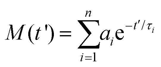 | (5) |
This modeling provides, for each considered wavelength, a collection of lifetimes (τi) and their amplitudes (ai), which are the starting point to conduct a global analysis. Essentially, the weighted average of this collection results in a single set of lifetimes that is employed to fit the transients at all probe wavelengths. The derived amplitudes ai(λ) are represented in the DAS (decay associated spectra) plot in Fig. 3.
Computational
EOM-CCSD calculations were performed with MOLPRO version 2022.3,46–48 CAM-B3LYP calculations with Gaussian1649 version A.03 and XMS-CASPT2 with MOLCAS50 version 23.06. The geometries were obtained at the CAM-B3LYP level of theory and validated to be minimum energy stationary points via computation of the geometrical Hessian matrix. The 6-311++G** basis set was used in all calculations. In the XMS-CASPT2 calculations an 8 electron 9 orbital active (8e,9o) space was used in conjunction with an ionization potential electron affinity (IPEA) shift of 0.25 a.u. Additionally, an imaginary shift of 0.20 a.u. was used to help avoid weakly intruding states.Results
Calculations
The first two vertical excitation energies (VEEs) for the most stable structures of the aniline(H2O)1 and aniline(CH3OH)1 clusters have been compared at different levels of theory: EOM-CCSD, CAM-B3LYP and XMS-CASPT2(8e,9o) (see Table S1, ESI†). For clarity, only the EOM-CCSD data has been provided in Table 1, while CAM-B3LYP and XMS-CASPT2(8e,9o) values are found in Table S1 (ESI†). Note that we show the CASSCF orbitals in the manuscript as they are cleaner for illustrative purposes than the EOM-CCSD ones. The two geometries calculated (Fig. 1) correspond to the solvent molecule interacting with the amino nitrogen (N⋯H–O) in isomer 1 (1-aniline), or the hydrogen (N–H⋯O) in isomer 2 (2-aniline), where the former is found to be the lowest energy arrangement of the two, with an energy separation of less than one tenth of an eV at the CCSD level of theory. For both solvents, the calculated S1 and S2 states exhibit either localized ππ* or πRydberg character. The Rydberg character is predominantly of s-type character. The ππ* or πRydberg character of the transition is indicated for each case (see Table 1).| Structure | S1 | S2 | S2–S1 [eV] | ||
|---|---|---|---|---|---|
| VEE [eV] (nm) | Character | VEE [eV] (nm) | Character | ||
| 1-aniline(H2O)1 | 5.17 (240) | ππ* | 5.39 (230) | πRydberg | 0.22 |
| 2-aniline(H2O)1 | 4.73 (262) | ππ* | 4.80 (258) | πRydberg | 0.07 |
| Aniline(H2O)2 | 4.93 (251) | ππ* | 5.36 (231) | πRydberg | 0.43 |
| Aniline(H2O)3 | 4.89 (254) | ππ* | 5.24 (237) | πRydberg | 0.35 |
| 1-aniline(CH3OH)1 | 4.92 (252) | ππ* | 5.37 (231) | πRydberg | 0.45 |
| 2-aniline(CH3OH)1 | 4.75 (261) | ππ* | 4.90 (253) | πRydberg | 0.15 |
| 1-aniline(CH3OH)2 | 4.90 (253) | ππ* | 5.35 (232) | πRydberg | 0.45 |
| 2-aniline(CH3OH)2 | 4.70 (264) | ππ* | 4.87 (255) | πRydberg | 0.17 |
| aniline(CH3OH)3 | 4.87 (255) | ππ* | 5.39 (230) | πRydberg | 0.52 |
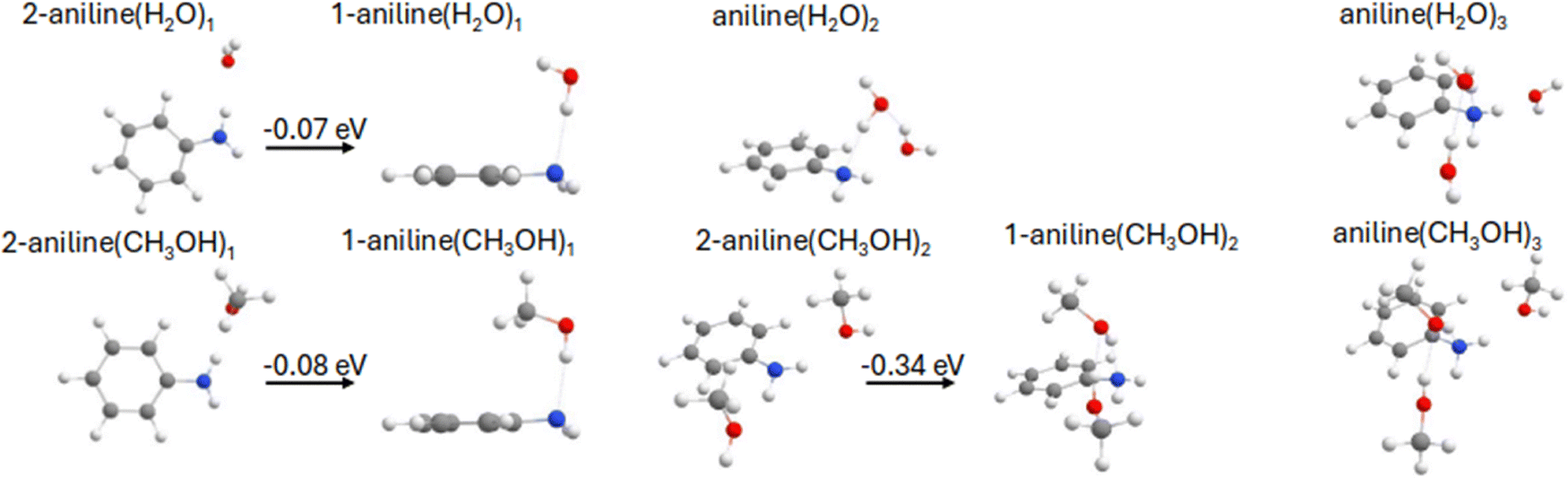 | ||
| Fig. 1 Geometries of various aniline–water and -methanol clusters computed using CAM-B3LYP. Where applicable, the energy difference between relevant conformations is also provided at the CCSD level of theory. | ||
For 1-aniline(H2O)1, the VEE of the S1 state is predicted to be 5.17 eV (240 nm) and of ππ* character while the VEE of S2 is 0.22 eV higher-lying (5.39 eV, 230 nm) and of πRydberg character. For 2-aniline(H2O)1, the ordering of the states is analogous to 1-aniline(H2O)1, however, the VEEs are drastically lowered to 4.73 and 4.80 eV, respectively. In 2-aniline(H2O)1, the energy separation of the S1 and S2 states is much lower at 0.07 eV compared to 0.22 eV observed in 1-aniline(H2O)1. XMS-CASPT2(8e,9o) agrees with the ordering of the ππ* and πRydberg states for both conformations. When using CAM-B3LYP, however, the ordering of the states inverts in 2-aniline(H2O)1, with the Rydberg state lower in energy.
For 1-aniline(CH3OH)1, the VEE of the S1 state is predicted to be 4.92 eV, which is 0.25 eV lower than the water counterpart. Once again, this state is of ππ* character with the πRydberg* state located at 5.37 eV. For 2-aniline(CH3OH)1, the VEE of the S1 and S2 states are 4.75 and 4.90 eV, respectively. For methanol, both XMS-CASPT2(8e,9o) and CAM-B3LYP agree with the EOM-CCSD ordering. As mentioned above, the Rydberg transition is of s-type character for all complexes and for small isovalues encapsulates the entire complex (see Fig. 2). Increasing the isovalue allows us to determine where most of the electron density resides. For 2-aniline(H2O)1, the majority of the density sits around the solvent molecule indicating a clear CT type transition. For 2-aniline(CH3OH)1, this is not the case as the electron density predominantly encapsulates the aniline. In contrast to the 2-aniline complexes, for 1-aniline most of the electron density is located around the amine moiety for both solvents, the VEEs of these complexes differ by only 0.02 eV.
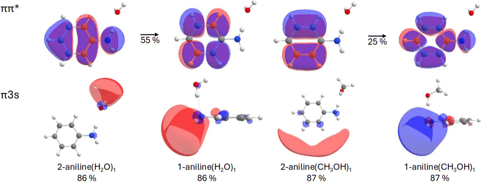 | ||
| Fig. 2 The important CASSCF orbitals for various aniline–water and -methanol clusters. For the ππ* transition, we show orbitals for the 2-aniline(H2O)1 complex only, but similar orbitals and transition character, the latter given as percentage, were found for the 3 other complexes. An isovalue of 0.02 hartree per bohr3 was used in all molecular orbital density plots. | ||
The inclusion of another solvent molecule into the system was also explored. For both water and methanol, a minimum was located which involved one solvent molecule interacting with the amino nitrogen (N⋯H–O) and the other solvent molecule interacting with the hydrogen (N–H⋯O), in addition to the interaction between the solvent molecules. For methanol we refer to this confirmation as 1-aniline(CH3OH)2 as another minimum was located for which both solvent molecules interact with the amino nitrogen on opposite sides (2-aniline(CH3OH)2), but this was found to be 0.34 eV higher in energy. For aniline–(H2O)2, only a single conformation was found, with the VEE of the S1 being 4.93 eV and of ππ* character. This is 0.24 eV below the equivalent state in 1-aniline(H2O)1 but 0.20 eV above 2-aniline(H2O)1. The VEE of the πRydberg state is relatively unchanged when compared to 1-aniline(H2O)1. For 1-aniline(CH3OH)2, which is the lower energy conformation, the VEE of S1 and S2 is 4.90 and 5.35 eV, respectively. This is very similar to the water counterpart. The inclusion of a third solvent molecule, thus fully saturating the hydrogen bonding network around the NH2 group, has little effect on the VEE of S1 for both solvents, which is also true for the VEE of S2 in aniline. The VEE of the S2 state in aniline(H2O)3, was lowered by 0.12 eV (5.36 eV) when compared to aniline(H2O)2.
Pump–probe TA experiments
Fig. 3 shows the TA data corresponding to the 267 and 200 nm excitations of aniline in methanol in the left- and right-hand columns, respectively. Based on previous measurements of aniline in other solvents,10,34 the spectra recorded at short times after the 267 nm excitation can be attributed to the excited state absorption (ESA) of the S1 ππ* state, with a maximum at 557 nm. This bright state relaxes along a photophysical pathway that includes ISC, with a lifetime of ∼3.0 ns,9,51 giving rise to a triplet state absorption (TSA) that is perceptible in our data as the band emerging at ∼415 nm in the longer time-scales. Consequently, the spectra recorded at the limit of the observation window (Fig. 3a1; 2 ns) are composed of the decaying ESA and the growing TSA. The lifetimes derived (Fig. 3b1) and their distributions across the WLC probe spectrum (Fig. 3c1) support this interpretation. While two small-amplitude functions with associated DAS lifetimes in the picosecond domain account for the solvent response and vibrational dynamics in the S1 state (τ1 = 0.7 ps and τ2 = 7.5 ps), relaxation is dominated by the ns decay of the ESA band, τ3 = 3.1 ns. Finally, the extremely long-lived τ1 > 10 ns component reproduces the background that matches the long-living TSA.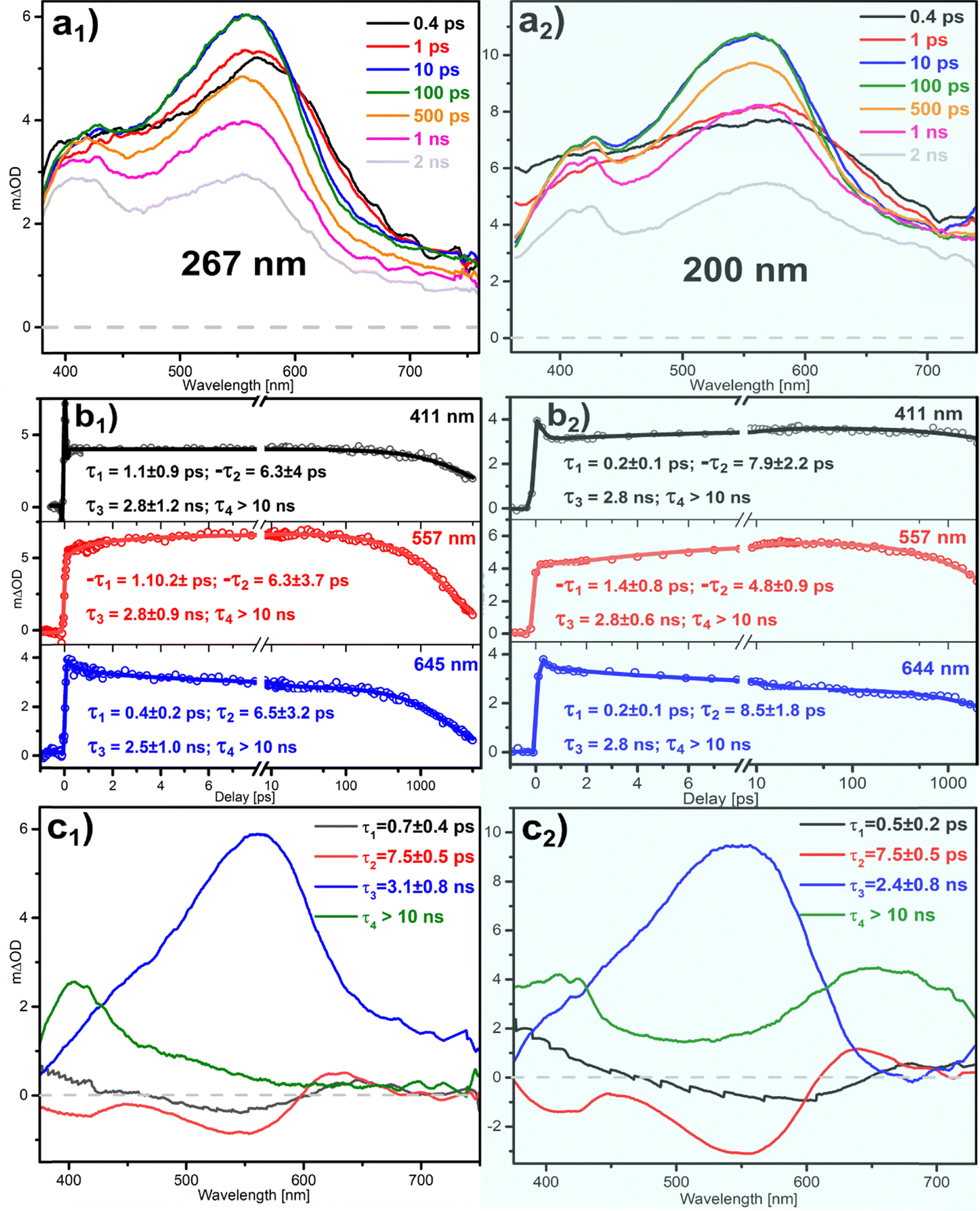 | ||
| Fig. 3 TA measurements of aniline in methanol exciting at 267 (left) and 200 nm (right). (ai) TA spectra recorded at selected pump–probe delays. (bi) Transients corresponding to the temporal evolution of the absorption at the indicated wavelengths. The lifetimes not including error bars were kept fixed in the fitting. (ci) DAS showing the distribution across the spectrum of the indicated temporal constants. These are obtained by averaging the constants derived from transients at selected individual probe wavelengths. | ||
Although the data for the 200 nm excitation can be reproduced by almost the exact same set of numerical time constants described above for the 267 nm case, the measurements show the presence of additional species in the spectra that indicate different relaxation channels. First, with respect to the 267 nm measurements, the series of spectra in Fig. 3a2 exhibit an enhanced absorption on the red side, around 700 nm. Second, a more structured band peaking at ∼415 nm develops after a few picoseconds and remains almost unchanged until the longest delays. These two features are clearly perceptible in the long τ4 component of the DAS, which reproduces the absorption spectra of aniline cations and solvated electrons.10,34 Therefore, the 200 nm excitation, in addition to preparing the ππ* excited state of the molecule reproduced by the τ3 = 2.4 ns component, induces the ionization of the molecule, as the presence of the cations and electrons in the long-time scale proves.
Pump–repump–probe experiments
To gain further insights, particularly into the ionization channel, pump–repump–probe experiments were conducted by using 550 (Fig. 4a) and 800 nm (Fig. S2, ESI†) repump pulses at a delay of 20 ps after the 267 nm pump. In both cases, the pump–repump spectra collected a few ps after the 267 nm excitation are characterized by a negative absorption caused by the bleach of the S1 ππ* state. Overlapping with this band, a positive contribution on both edges of the spectrum that corresponds to the absorption of cations and ejected electrons is also perceptible. The bleach band recovers in a few ps, and only the features assigned to the ionization persist in the long term. These results evidence that the absorption of the repump pulse at both wavelengths used induces the ionization of the initially prepared S1 ππ* state. The magnitude of the signal is, however, much higher in the case of the 550 nm repump, as at this wavelength the absorption of the S1 state is at a maximum. | ||
| Fig. 4 (a) Pump (267 nm)–repump (550 nm)–probe spectra collected for aniline in methanol at fixed pump–repump delay (Δt1 = 20 ps) and at the indicated repump–probe delays (Δt2). (b) Transient corresponding to the evolution of the pump–repump–probe signal as a function of the pump–probe delay (Δt2) at the 586 nm probe wavelength. The dots correspond to the experimental data and the solid lines are the obtained multiexponential fits. | ||
Fig. 4b shows the transients derived from the spectra at the 586 nm probe wavelength. At this wavelength, the S1 ππ* state, and the pre- and fully solvated electrons absorb. Essentially, the signals are composed of a negative portion (bleach of the S1 state) that recovers with a few ps lifetime, followed by the positive ionization signal, which partially decays in hundreds of picoseconds to form the final long-lasting absorption of the solvated electrons. This decay can be assigned to cation-electron recombination processes that occur after the evolution from the pre- to fully-solvated electrons.52–55 In the 800 nm repump experiments (Fig. S2, ESI†), the small absorption signal obtained precludes us from obtaining meaningful temporal constants, however, the spectral features agree with the 550 repump experiments. The recombination decay is less perceptible for the experiments with the 800 nm repump, due to the smaller amount of charged species produced in this instance, but the overall behavior is analogous to the 550 nm repump case.
Discussion
267 nm excitation
Fig. 5 shows the different species remaining in the methanol solution in the long-time limit following 267 and 200 nm excitation and permits identification of their characteristic absorption spectra. These agree with previous observations on the absorptions of aniline triplet states, cations and electrons formed in water.10 While the long-term absorption at 267 nm (red trace) corresponds to triplet states of the aniline molecule, the pump(267 nm)–repump(800 nm) experiment (blue trace) yields, exclusively, the absorptions of the charged species. The sum of both traces, after scaling by an appropriate factor (green trace), matches the absorption spectra obtained at 200 nm (black trace). Therefore, contrary to what is observed in water and in methanol at 200 nm, the excitation of aniline in methanol at 267 nm does not induce ionization of the molecule. Furthermore, differently to the 200 nm case, the TA spectra collected right after the excitation (Fig. 3a1 black trace) can be assigned exclusively to the absorption of the aniline S1 ππ* state. The evolution of the system is characterized by the temporal constants of Fig. 3b1 and c1, where τ1 and τ2 account for the solvent response and vibrational cooling on the excited state, respectively, and τ3 reflects the relaxation of the S1 ππ* state. Although the form of the τ3 DAS (Fig. 3c1) seems to reproduce the absorption of this state, it must be noted that it should also describe the absorption of the forming triplet state. The positive amplitude of the lifetime across the spectrum indicates that the decaying process dominates. Finally, the distribution of the background τ4 matches the absorption of the long-living triplet states, which are the only absorbing species found in the medium in the long-time limit.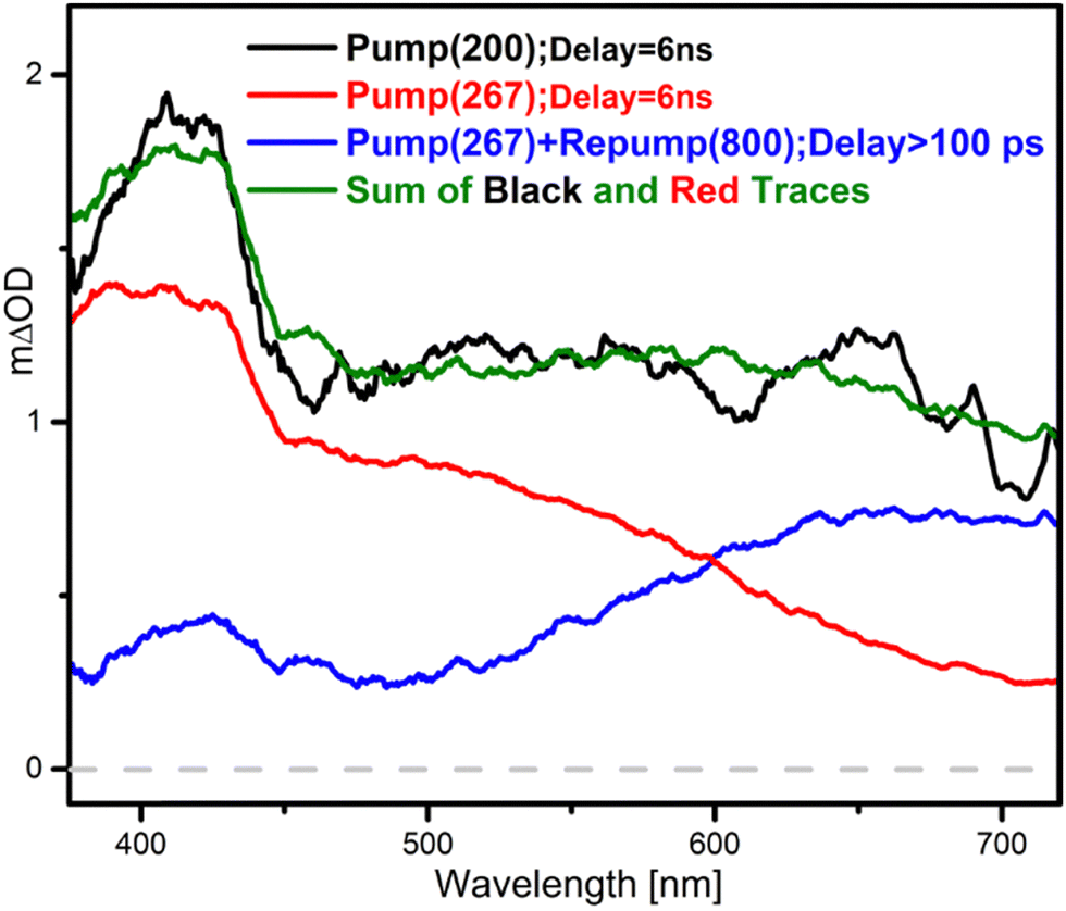 | ||
| Fig. 5 Interpretation of the absorption spectrum obtained for aniline in methanol at long pump–probe delays, after 200 nm excitation (black trace), as the scaled sum (green trace) of the contributions corresponding to aniline cations and solvated electrons (blue trace) and neutral aniline in triplet states (red trace). The former corresponds to a pump(267 nm)–repump(800 nm) experiment, while the latter is a long delay spectrum from the 267 nm pump TA experiment. See text for details. | ||
From these data we can conclude that no charged species, nor precursors of them, are formed within the experimental time-resolution (∼250 fs) during the relaxation process following 267 nm absorption. The pump–repump experiments carried out by re-exciting the initially prepared excited state with 550 or 800 nm pulses after 20 ps confirm this. Of note here is the observation that, after re-pumping at Δτ1 = 20 ps with both 550 and 800 nm, the bleach band obtained shortly after the re-excitation matches the absorption of the S1 ππ* state (Fig. 4a and Fig. S2, ESI†). This indicates that following 267 nm excitation, the only absorbing state – even at the red end of the probe spectrum – is S1 ππ*. This is in clear contrast to what we observed previously in water at the same pump wavelength.34
In order to rationalize this observation, we must consider the influence of the solvent on the IP of the solute molecule, which is a very complex question. A first aspect to contemplate is the different polarity that both solvents present. In the work by West et al.56 the photoelectron spectrum of aniline in water and methanol jets is compared. Although methanol is less polar than water, the first ionization bands are centered at alike positions in both solvents, ∼7.5 eV (IPv) and seem to extend toward comparable lower energies, ∼6.0 eV, which points to a similar effect of the solvent on the formation of electrons in the conduction band of solution. However, to understand the absence in methanol solutions of the ionization channel found in water, it is important to consider the ionization mechanism at low energies, below the solvent conduction band, which requires a microscopic view of the solute–solvent interaction. In the case of aniline34 and other aromatic molecules26,32,33 the photoionization at energies as low as ∼4.5 eV, well below the water conduction band,16,57,58 has been proposed to be mediated by the formation of a CT state or cation-electron contact ion-pair.24 The absorption signature and the dynamics (from hundreds ps to ns) have been characterized for this precursor state in the case of aniline and indole in water.26,34 This CT state has been theoretically described as a πσ* in nature, where the σ* orbital presents Rydberg character and is located on the solvent molecules that interact with the N–H group of the molecule.29,31,32 Although this state is optically dark at 267 nm, it could be indirectly populated by coupling to the lowest ππ* excitation in aniline. In fact, Kumar et al.26 have found for indole water solutions that after its formation, the ion-contact pair remains in equilibrium with the ππ* (La) state.
Contrary to the water case, the observations we have collected for aniline in methanol do not show any sign of ionization. Assuming the above-described mechanism, the lack of ionization could be ascribed to the inaccessibility of the CT character πσ* state. In fact, in contrast to water, the pump–repump–probe experiments in methanol do not show the formation of this state. In order to shed some light on this different behavior, we can compare the calculations described above for the aniline(H2O)n and aniline(CH3OH)n clusters. The first idea we can extract from this set of data is that the clusters with more than one solvent molecule do not essentially change the picture derived from the mono-solvated species, and accordingly, we will focus mainly on the latter. For both solvents, the same two structures are found: with the solvent interacting with the nitrogen, N⋯H–O (1-aniline), or the hydrogen, N–H⋯O (2-aniline). Although the former is slightly more stable, the latter preferentially stabilizes the S2 πRydberg state. The most significant difference between the two solvents, however, is the character of this S2 πRydberg state. For the water cluster with the N–H⋯O interaction, the stabilized πRydberg dominant state shows a CT character, involving the solvent molecule (Fig. 2). Contrarily, in the analogous methanol geometry the S2 πRydberg state does not exhibit CT character, as it mostly involves the aromatic ring of the aniline molecule. This result leads us lead us to suggest that the effect of the specific N–H⋯O interaction on the electronic structure can be behind the different behavior, regarding the photoionization channel, found between water and methanol. It is important to remark here the limitations of a model based on the interaction with a single solvent molecule, which ignores other interactions between aniline and water, and the bulk effect of the solvent. Therefore, although for a related system as aqueous indole, it has been shown that the N–H⋯O interaction by itself can account for the specific solvent effect,59 further theoretical modelling, in particular, by methods able to consider the effect of additional solvent–solute interactions would be required to test the validity of these ideas.
200 nm excitation
As shown in Fig. 3a2–c2, excitation at 200 nm clearly yields solvated cations and electrons in addition to the long-living triplet states of the neutral molecule. It is important to note that although we cannot quantify the relative quantum yields, the small absorption signal measured at long delays (Fig. 3a2–c2) and the large cross section of the solvated electron absorption,41,60,61 lead us to conclude that the ionization yield is fairly small. As already mentioned above, the numerical time constants retrieved from the TA spectra modelling are very similar to those obtained at 267 nm. This seems to indicate that none of them are related with the ionization process. In methanol, the absorption at 200 nm (∼6.2 eV) excites the aniline molecule via the S0(π)-31ππ* transition, which carries a high oscillator strength.62–64 There are, however, no time-resolved observations regarding the relaxation of this 31ππ* state,40,64,65 as it presumably undergoes internal conversion to the lower S1 ππ* state in tens of fs (i.e. well within the pump–probe correlation time). Hence, the prompt spectrum in Fig. 3a2 (black trace) likely corresponds to the absorption of a vibrationally hot S1 state that will evolve towards the ESA band observed at 267 nm with the τ1 and τ2 lifetimes. As discussed earlier, these reflect the solvent response and vibrational cooling, respectively. As the DAS in Fig. 3c2 shows, the ESA band characterized by the 2.4 ns S1 ππ* absorption extends across most of the probed spectrum. On the blue and red edges, however, the observed signal remains almost constant between the earliest pump–probe time delays and the final measurement after 2 ns. These regions correspond to the cation and electron bands, since they seem to be formed immediately after the 200 nm excitation and do not appear to exhibit any lifetime associated with their formation. Remarkably, the electron absorption on the red portion does not show the characteristic dynamics observed in water excited at 267 nm, pointing to a different ionization route.The pump–repump data can provide some additional insights regarding the ionization channel. The combined absorption of the 267 nm pump and 800 nm repump yields a total excitation energy of 6.2 eV, which as with the case of 200 nm photons (also 6.2 eV) would prepare the 31ππ* state. On the other hand, with the 550 nm repump, the 6.9 eV total pump + re-pump excitation must lead to the next 41ππ* excitation, for which an even larger oscillator strength is predicted.63 The pump–repump spectra are very similar at both repump wavelengths. Immediately after the re-excitation, they show the bleach of the S1 ππ* state recovering in few ps. This is a clear sign any higher lying ππ* states that are accessed undergo internal conversion back to the S1 state after this time. As already mentioned above, the internal conversion to the lower S1 ππ* state is presumed to occur in a few tens of fs. Hence, the observed recovery of the bleach must account for the subsequent cooling of the formed S1 ππ* state. This is the same process observed in the regular (i.e. no repump) TA experiments at 200 nm, and accordingly, the derived τ1 and τ2 lifetimes are very similar. Furthermore, in agreement with the TA data, the positive contributions of the electrons and geminate partner cations are also perceptible in the prompt bleach band, meaning that they are formed simultaneously or immediately (below our temporal resolution) after populating the 31ππ*/41ππ* excited state of the neutral aniline. At this energy, the formation of the latter is therefore likely to occur in parallel with the direct ionization of the molecule. A similar mechanism has been proposed for the ionization observed for indole in water at 200 nm.26 The pump–repump transients (Fig. 4b) at the electron absorption band (586 nm), show a distinctive decay in hundreds of ps that can be assigned to recombination with the counterpart cations.34 The recombination processes are distinctive of the formation of solvated electrons from the pre-solvated or trapped electrons and have been observed at similar rates in the ionization of water and methanol at energies below and above the bottom edge of the solvent conduction band.52–55
Conclusions
A combination of transient absorption spectroscopy experiments, conducted with fs resolution, and complementary excited state calculations provide a comprehensive view of the relaxation channels of aniline in methanol following UV absorption. After excitation at 267 nm, the observed dynamics in methanol, can be fully interpreted in terms of the formation of a bright ππ* state and the subsequent relaxation following a photophysical pathway that leads, in the probed observation window, to the formation of triplet states with a ∼3.0 ns lifetime. Very remarkably, the spectra observed at long delays reveal no indication of charged species remaining in the solution, while the transient data show no hint of the formation of a CT state precursor of the ion. This result contrasts with the observations collected for aniline in aqueous medium. There, the photoionization of the molecule through a precursor CT state formed in parallel or shortly after the excitation along the bright ππ* excitation has been shown.34Based on the conducted excited state calculations on aniline(H2O)1 and aniline(CH3OH)1 clusters, we suggest that the absence of this ionization mechanism in methanol could be attributed to the different nature that the lowest Rydberg character πσ* state exhibits. In the case the of water, as a consequence of the N–H⋯O interaction, the σ* is localized on the solvent molecule – as seen in our calculations on the 2-aniline(H2O)1 cluster. This is not the case, however, for the computed equivalent state in the analogous 2-aniline(CH3OH)1 cluster, which being localized on the aromatic ring, does not exhibit the CT character required to mediate the ionization process. The picture extracted from this very simplistic model should be contrasted with the results from more detailed descriptions of the solute–solvent systems.
On the other hand, the experiments carried out using 200 nm excitation show the presence of cations and electrons in the methanol solution. The time-dependent data indicate that ionization occurs immediately after the excitation (i.e. below the temporal resolution of the present measurements), and the formation of the fully solvated electrons is mediated by the characteristic recombination process. Consequently, as has been reported in the aqueous medium at the same energy, the ionization occurs through a conventional mechanism where the electron is ejected directly into the solvent.
Conflicts of interest
There are no conflicts to declare.Data availability
Data for this article, including experimental data corresponding to Fig. 3, 4, 5 and Fig. S1 (ESI†) are available at Science Data Bank at https://www.scidb.cn/en/s/2U3iUv (provisional).Acknowledgements
The experimental work was funded by the Spanish MICINN through the grant: PID2021-127918NB-I00 and the Basque Government (IT1491-22). I.L. thanks the UPV/EHU and the Basque Government for his pre- and postdoctoral fellowships. Technical and human support provided by SGIker (UPV/EHU, MICINN, GV/EJ, ESF) is also gratefully acknowledged. MJP and DT thank the Engineering and Physical Sciences Research Council (EPSRC) for grants EP/P001459, EP/R030448, EP/V006746, and EP/T021675. AWP and MJP also gratefully acknowledge the Leverhulme Trust through research project grant RPG-2020-208.References
- T. Schultz, E. Samoylova, W. Radloff, I. V. Hertel, A. L. Sobolewski and W. Domcke, Science, 2004, 306, 1765–1768, DOI:10.1126/science.1104038.
- S. D. Camillis, J. Miles, G. Alexander, O. Ghafur, I. D. Williams, D. Townsend and J. B. Greenwood, Phys. Chem. Chem. Phys., 2015, 17, 23643–23650, 10.1039/C5CP03806E.
- R. Improta, F. Santoro and L. Blancafort, Chem. Rev., 2016, 116, 3540–3593, DOI:10.1021/acs.chemrev.5b00444.
- E. J. Land and G. Porter, Trans. Faraday Soc., 1963, 59, 2027–2037, 10.1039/TF9635902027.
- J. Yang, PATAI'S Chemistry of Functional Groups, John Wiley & Sons, Ltd, 2009 Search PubMed.
- S. Suzuki and T. Fujii, Bull. Chem. Soc. Jpn., 1975, 48, 835–840, DOI:10.1246/bcsj.48.835.
- T. Ebata, C. Minejima and N. Mikami, J. Phys. Chem. A, 2002, 106, 11070–11074, DOI:10.1021/jp021457t.
- B. N. Rajasekhar, A. Veeraiah, K. Sunanda and B. N. Jagatap, J. Chem. Phys., 2013, 139, 064303, DOI:10.1063/1.4817206.
- S. Tobita, K. Ida and S. Shiobara, Res. Chem. Intermed., 2001, 27, 205–218, DOI:10.1163/156856701745087.
- F. Saito, S. Tobita and H. Shizuka, J. Chem. Soc., Faraday Trans., 1996, 92, 4177–4185, 10.1039/FT9969204177.
- F. Saito, S. Tobita and H. Shizuka, J. Photochem. Photobiol., A, 1997, 106, 119–126, DOI:10.1016/S1010-6030(97)00048-8.
- Y. Matsumura, K. Iida and H. Sato, Chem. Phys. Lett., 2013, 584, 103–107, DOI:10.1016/j.cplett.2013.08.081.
- T. Ogawa, T. Ogawa and K. Nakashima, J. Phys. Chem. A, 1998, 102, 10608–10613, DOI:10.1021/jp982220t.
- L. I. Grossweiner, G. W. Swenson and E. F. Zwicker, Science, 1963, 141, 805–806, DOI:10.1126/science.141.3583.805.
- H. Joschek and L. I. Grossweiner, J. Am. Chem. Soc., 1966, 88, 3261–3268, DOI:10.1021/ja00966a017.
- D. Grand, A. Bernas and E. Amouyal, Chem. Phys., 1979, 44, 73–79, DOI:10.1016/0301-0104(79)80064-6.
- R. J. Robbins, G. R. Fleming, G. S. Beddard, G. W. Robinson, P. J. Thistlethwaite and G. J. Woolfe, J. Am. Chem. Soc., 1980, 102, 6271–6279, DOI:10.1021/ja00540a016.
- J. Zechner, G. Köhler, N. Getoff, I. Tatischeff and R. Klein, Photochem. Photobiol., 1981, 34, 163–168, DOI:10.1111/j.1751-1097.1981.tb08980.x.
- E. Amouyal, A. Bernas, D. Grand and J. Mialocq, Faraday Discuss. Chem. Soc., 1982, 74, 147–159, 10.1039/DC9827400147.
- J. C. Mialocq, E. Amouyal, A. Bernas and D. Grand, J. Phys. Chem., 1982, 86, 3173–3177, DOI:10.1021/j100213a022.
- Y. Hirata, N. Murata, Y. Tanioka and N. Mataga, J. Phys. Chem., 1989, 93, 4527–4530, DOI:10.1021/j100348a027.
- P. S. Sherin, O. A. Snytnikova and Y. P. Tsentalovich, Chem. Phys. Lett., 2004, 391, 44–49, DOI:10.1016/j.cplett.2004.04.068.
- P. S. Sherin, O. A. Snytnikova, Y. P. Tsentalovich and R. Z. Sagdeev, J. Chem. Phys., 2006, 125, 144511, DOI:10.1063/1.2348868.
- J. Peon, G. C. Hess, J. L. Pecourt, T. Yuzawa and B. Kohler, J. Phys. Chem. A, 1999, 103, 2460–2466, DOI:10.1021/jp9840782.
- G. Kumar, A. Roy, R. S. McMullen, S. Kutagulla and S. E. Bradforth, Faraday Discuss., 2018, 212, 359–381, 10.1039/C8FD00123E.
- G. Kumar, M. Kellogg, S. Dey, T. A. A. Oliver and S. E. Bradforth, J. Phys. Chem. B, 2024, 128, 4158–4170, DOI:10.1021/acs.jpcb.4c01223.
- T. A. A. Oliver, Y. Zhang, A. Roy, M. N. R. Ashfold and S. E. Bradforth, J. Phys. Chem. Lett., 2015, 6, 4159–4164, DOI:10.1021/acs.jpclett.5b01861.
- J. W. Riley, B. Wang, J. L. Woodhouse, M. Assmann, G. A. Worth and H. H. Fielding, J. Phys. Chem. Lett., 2018, 9, 678–682, DOI:10.1021/acs.jpclett.7b03310.
- A. L. Sobolewski and W. Domcke, Chem. Phys. Lett., 2000, 329, 130–137, DOI:10.1016/S0009-2614(00)00983-0.
- A. L. Sobolewski and W. Domcke, J. Phys. Chem. A, 2001, 105, 9275–9283, DOI:10.1021/jp011260l.
- A. L. Sobolewski, W. Domcke, C. Dedonder-Lardeux and C. Jouvet, Phys. Chem. Chem. Phys., 2002, 4, 1093–1100 RSC.
- M. Wohlgemuth, V. Bonacic-Koutecký and R. Mitric, J. Chem. Phys., 2011, 135, 054105, DOI:10.1063/1.3622563.
- I. Sandler, J. J. Nogueira and L. González, Phys. Chem. Chem. Phys., 2019, 21, 14261–14269, 10.1039/C8CP06656F.
- I. Lamas, J. González, A. Longarte and R. Montero, J. Chem. Phys., 2023, 158, 191102, DOI:10.1063/5.0147503.
- A. L. Sobolewski and W. Domcke, Chem. Phys. Lett., 2000, 321, 479–484, DOI:10.1016/S0009-2614(00)00404-8.
- A. Kumar, M. Kołaskia and K. S. S. Kim, J. Chem. Phys., 2008, 128, 034304, DOI:10.1063/1.2822276.
- I. Frank and K. Damianos, Chem. Phys., 2008, 343, 347–352, DOI:10.1016/j.chemphys.2007.08.029.
- R. Spesyvtsev, O. M. Kirkby and H. H. Fielding, Faraday Discuss., 2012, 157, 165–179, 10.1039/C2FD20076G.
- R. Spesyvtsev, O. M. Kirkby, M. Vacher and H. H. Fielding, Phys. Chem. Chem. Phys., 2012, 14, 9942–9947, 10.1039/C2CP41785E.
- J. O. F. Thompson, L. Saalbach, S. W. Crane, M. J. Paterson and D. Townsend, J. Chem. Phys., 2015, 142, 114309, DOI:10.1063/1.4914330.
- E. J. Hart and J. W. Boag, J. Am. Chem. Soc., 1962, 84, 4090–4095, DOI:10.1021/ja00880a025.
- R. E. Larsen, W. J. Glover and B. J. Schwartz, Science, 2010, 329, 65–69, DOI:10.1126/science.1189588.
- Y. Hu and E. R. Bernstein, J. Phys. Chem. A, 2009, 113, 639–643, DOI:10.1021/jp807049e.
- T. Watanabe and K. Ohashi, Comput. Theor. Chem., 2022, 1215, 113850, DOI:10.1016/j.comptc.2022.113850.
- B. Dietzek, T. Pascher, V. Sundström and A. Yartsev, Laser Phys. Lett., 2007, 4, 38 CrossRef.
- T. Korona and H. Werner, J. Chem. Phys., 2003, 118, 3006–3019, DOI:10.1063/1.1537718.
- H. Werner, P. J. Knowles, G. Knizia, F. R. Manby and M. Schütz, WIREs Comput. Mol. Sci., 2012, 2, 242–253, DOI:10.1002/wcms.82.
- H. Werner, P. J. Knowles, F. R. Manby, J. A. Black, K. Doll, A. Heßelmann, D. Kats, A. Köhn, T. Korona, D. A. Kreplin, Q. Ma, T. F. Miller, I. I. I. A. Mitrushchenkov, K. A. Peterson, I. Polyak, G. Rauhut and M. Sibaev, J. Chem. Phys., 2020, 152, 144107, DOI:10.1063/5.0005081.
- M. Frisch, G. W. Trucks and H. B. Schlegel, et al., Gaussian16 Rev. A.03, Gaussian Inc., Wallingford, CT, 2016 Search PubMed.
- G. Karlström, R. Lindh, P. Malmqvist, B. O. Roos, U. Ryde, V. Veryazov, P. Widmark, M. Cossi, B. Schimmelpfennig, P. Neogrady and L. Seijo, Comput. Mater. Sci., 2003, 28, 222–239, DOI:10.1016/S0927-0256(03)00109-5.
- G. Köhler, J. Photochem., 1987, 38, 217–238, DOI:10.1016/0047-2670(87)87019-3.
- R. A. Crowell and D. M. Bartels, J. Phys. Chem., 1996, 100, 17940–17949, DOI:10.1021/jp9610978.
- L. Turi, P. Holpár and E. Keszei, J. Phys. Chem. A, 1997, 101, 5469–5476, DOI:10.1021/jp970174b.
- V. H. Vilchiz, X. Chen, J. A. Kloepfer and S. E. Bradforth, Radiat. Phys. Chem., 2005, 72, 159–167, DOI:10.1016/j.radphyschem.2004.06.013.
- M. H. Elkins, H. L. Williams and D. M. Neumark, J. Chem. Phys., 2015, 142, 234501, DOI:10.1063/1.4922441.
- C. W. West, J. Nishitani, C. Higashimura and T. Suzuki, Mol. Phys., 2021, 119, e1748240, DOI:10.1080/00268976.2020.1748240.
- T. Goulet, A. Bernas, C. Ferradini and J. Jay-Gerin, Chem. Phys. Lett., 1990, 170, 492–496, DOI:10.1016/S0009-2614(90)87090-E.
- J. M. Jung and H. Gress, Chem. Phys. Lett., 2002, 359, 153–157, DOI:10.1016/S0009-2614(02)00707-8.
- L. He, L. Tomaník, S. Malerz, F. Trinter, S. Trippel, M. Belina, P. Slavíček, B. Winter and J. Küpper, J. Phys. Chem. Lett., 2023, 14, 10499–10508, DOI:10.1021/acs.jpclett.3c01763.
- F. Jou and G. R. Freeman, J. Phys. Chem., 1977, 81, 909–915, DOI:10.1021/j100524a021.
- F. Messina, M. Prémont-Schwarz, O. Braem, D. Xiao, V. S. Batista, E. T. J. Nibbering and M. Chergui, Angew. Chem., Int. Ed., 2013, 52, 6871–6875 CrossRef CAS PubMed.
- S. K. Sarkar and G. S. Kastha, Spectrochim. Acta, Pt. A: Mol. Spectrosc., 1992, 48, 1611–1624, DOI:10.1016/0584-8539(92)80235-O.
- Y. Honda, M. Hada, M. Ehara and H. Nakatsuji, J. Chem. Phys., 2002, 117, 2045–2052, DOI:10.1063/1.1487827.
- G. M. Roberts, C. A. Williams, J. D. Young, S. Ullrich, M. J. Paterson and V. G. Stavros, J. Am. Chem. Soc., 2012, 134, 12578–12589, DOI:10.1021/ja3029729.
- R. Montero, Á. P. Conde, V. Ovejas, R. Martínez, F. Castaño and A. Longarte, J. Chem. Phys., 2011, 135, 054308, DOI:10.1063/1.3615544.
Footnote |
| † Electronic supplementary information (ESI) available. See DOI: https://doi.org/10.1039/d5cp00937e |
| This journal is © the Owner Societies 2025 |