
Quantifying anomalous chemical diffusion through disordered porous rock materials†
Ashish
Rajyaguru
 *ab,
Ralf
Metzler
cd,
Andrey G.
Cherstvy
c and
Brian
Berkowitz
b
*ab,
Ralf
Metzler
cd,
Andrey G.
Cherstvy
c and
Brian
Berkowitz
b
aPaul Scherrer Institut, 5232 Villigen, Switzerland. E-mail: ashish.rajyaguru90@gmail.com
bDepartment of Earth and Planetary Sciences, Weizmann Institute of Science, Rehovot 7610001, Israel
cInstitute for Physics & Astronomy, University of Potsdam, 14476 Potsdam, Germany
dAsia Pacific Centre for Theoretical Physics, Pohang 37673, Republic of Korea
First published on 8th April 2025
Abstract
Fickian (normal) diffusion models show limitations in quantifying diffusion-controlled migration of solute species through porous rock structures, as observed in experiments. Anomalous diffusion prevails and can be interpreted using a Continuous Time Random Walk (CTRW) framework with a clear mechanistic underpinning. From the associated fractional diffusion equation we derive solutions over a broad range of anomalous diffusion behaviours, from highly anomalous to nearly Fickian, that yield temporal breakthrough curves and spatial concentration profiles of diffusing solutes. We illustrate that these solutions can be tailored to match realistic experimental conditions and resulting measurements that display anomalous diffusion. In particular, our analysis enables clear differentiation between early-time Fickian and anomalous diffusion, which becomes more pronounced over longer durations. It is shown that recent measurements of diffusion in natural rocks display distinct anomalous behaviour, with significant implications for critical assessment of solute migration in diverse geological and engineering applications.
1 Introduction
Mass transport of dissolved solutes is crucial in geological, biological, and engineering contexts. Mass transport that is subject to advection in a host liquid—chemical transport—is evident in scenarios such as contaminant release during aquifer recharge, drainage, or discharge cycles,1–5 and in the displacement of hydrocarbons from fractured rock networks.6 Conversely, in the absence of a velocity, diffusion governs the migration dynamics of dissolved solutes. Studies have shown that diffusion-dominated processes play a pivotal role in systems that involve molecular transport in microorganisms and dense liquids,7 the dispersion of contaminants in freshwater systems,8 nutrient migration in soils and root uptake,9 long-term performance of solid electrolytes and fuel cells,10,11 subsurface radioactive waste disposal,12 CO2 sequestration,13 biomineralisation,14 the weathering of heritage sites,15 and hydrogen storage.16,17A common denominator in these studies is that the intricate interactions between the properties of porous materials and solute species dictate the nature of chemical diffusion in a porous medium.18 Disordered porous media can induce complex local dynamics, such as heterogeneous travel times within the pore network, solute entrapment in dead-end pores, surface adsorption on pore walls, and/or consumption via sink terms. These localised phenomena significantly affect the initial solute distribution within the porous matrix, the local residence times, and the subsequent temporal release.
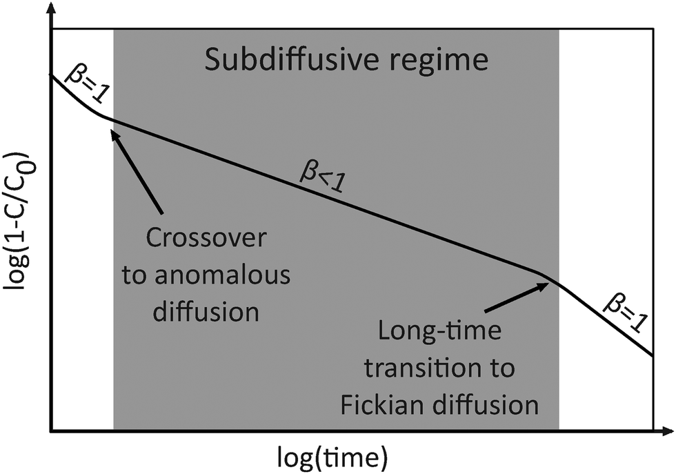
In the past two decades, biophysical research has provided compelling evidence that the interaction of solutes with heterogeneous porous media leads to “anomalous diffusion” behaviours that deviate from classical Fickian diffusion. Deviations from Fickian diffusion are exhibited during subdiffusion of mRNA within densely packed cytoplasmic membranes of E. coli, macromolecule dynamics in cell membranes and gels, and pathways for drug delivery in cerebral extracellular spaces.19–24 And yet, in contrast, chemical diffusion in geological studies has been—and generally continues to be—assumed to adhere to classical Fickian principles. Simulation studies demonstrating anomalous diffusion in porous media are typically hampered by the multiple scales necessary for its description. Concretely, molecular dynamics simulations demonstrate that anomalous diffusion arises for Ag+ ions and doxorubicin drug molecules interacting with silica surfaces.25,26 How to bridge scales in simulation approaches is discussed in Bousige et al.,27 albeit without the occurrence of anomalous diffusion—this would likely emerge for more pronounced tracer–surface interactions as shown in the above citations. With Monte Carlo simulations, anomalous diffusion is known to persist in effective models for porous structures based on random fractal structures of percolation clusters;28,29 see also NMR experiments using such structures.30 A recent experimental study presented high-resolution datasets that examined bromide diffusion through several natural chalk and dolomite rock samples, revealing that the long-time pattern of bromide diffusion exhibited distinctly non-Fickian, anomalous, behaviour.31
Measurements to assess and quantify diffusion-controlled solute migration in (generally water-saturated) porous materials, particularly in naturally heterogeneous rock samples, typically rely on a constant concentration inlet source to induce diffusive migration through an effectively (macroscopically) one-dimensional domain, with measurements of concentration at the outlet over time, known as “breakthrough curves (BTCs)”. In this context, Metzler et al. (2022)32 proposed that the Continuous Time Random Walk (CTRW) framework can be used to derive anomalous diffusion solutions and corresponding BTCs. The CTRW accounts for solute spreading with immobilisation times τ distributed according to a power-law probability density function (PDF) that, at long times, scales as ψ(τ) ≃ τ−1−β.‡ Here the scaling exponent 0 < β ≤ 1 controls the degree of deviation from Fickian diffusion (β = 1). Metzler et al. (2022)32 outlined a mathematical approach to evaluate BTC and flux solutions for anomalous diffusion across a range of β values, developing asymptotic solutions for long-time behaviour, and a full BTC solution for the special case of  .
.
The present study focuses on (i) developing semi-analytical solutions that yield full BTC and spatial concentration profiles over the range 0 < β ≤ 1, and then (ii) applying these quantitative tools to fully quantify and interpret measurements of diffusion in unique rock core experiments.31 To illustrate the differences between anomalous and Fickian diffusion, we present the BTC and flux solutions representing solute diffusion through macroscopically one-dimensional porous domains under constant inlet and semi-infinite outlet boundary conditions. We demonstrate the ability of the CTRW-based solutions to quantify the experimental measurements and show how β controls both the initial arrival times and long-time tailing of the BTC and flux solutions, distinct from Fickian diffusion behaviour. Finally, we highlight the disparity between large-scale chemical diffusion described by Fickian and anomalous models, emphasising the significance of considering anomalous diffusion in geological systems and its implications for critical interpretation of diffusion-driven processes in subsurface zones.
2 Anomalous diffusion model
In a seminal 1905 paper, Einstein investigated the physical mechanisms that cause the random motion of particles suspended in fluids, also known as Brownian motion;33 he postulated that these erratic movements arise from the continuous bombardments by thermalised water molecules.34 Drawing on the principles of the central limit theorem, he proposed the existence of a finite correlation time beyond which the displacement of particles becomes statistically independent and identically distributed. Einstein introduced the concept of the mean squared displacement (MSD) to describe the average distance a particle can travel freely before encountering neighbouring particles. Further insight into diffusion and their connection to chemical reactions was provided by Smoluchowski.35Building on these foundational concepts, Einstein arrived at the famous diffusion equation and thereby linked Brownian motion to the macroscopic spreading of particles:
 | (1) |
 | (2) |
 to obtain the MSD.19 In this case, the MSD shows that particle spreading via Brownian motion evolves linearly with time.
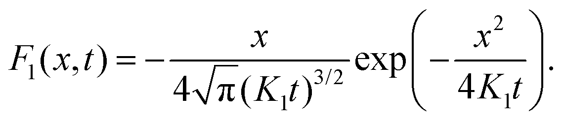
The theory of anomalous diffusion is based on a large variety of different stochastic models, depending on the physical mechanisms underlying the observed dynamics.19 One of the most important anomalous diffusion models is the CTRW framework, that models subdiffusion processes with anomalous diffusion exponent 0 < β ≤ 1 for a scale-free immobilisation time PDF of the form ψ(τ) ≃ τ−1−β.19,36 Unlike Brownian motion, the spreading of particles in a fixed lattice, under anomalous diffusion, is characterised by a power-law relationship between the MSD and time given by 〈x2(t)〉 ≃ tβ. For example, power law waiting time densities and power law MSDs were measured in porous media using a single-particle tracking approach.37 Mathematically, the behaviour of the PDF for such scale-free CTRWs in the hydrodynamic limit is governed by the time-fractional diffusion equation36
 | (3) |
 is defined in the Riemann–Liouville sense as
 | (4) |
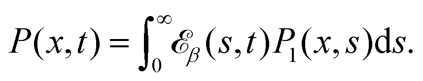
Based on the fractional diffusion eqn (3) the PDF P(x,t) can be obtained via the subordination method, translating the “operational time” s into the laboratory time t,§ that can be phrased as an integral relation of the form32,36,39
 | (5) |
 is given by the modified one-sided Lévy-stable PDF36
 | (6) |
 , β assumes the simple Lévy-Smirnov form32,36
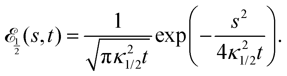 | (7) |
 was presented in Metzler et al. (2022).32
Fig. 1 compares the particle spreading from a point source into an unbounded space due to Brownian and anomalous diffusion. These solutions were derived by setting t = 5 and allowing x to vary between −5 and 5 for the Brownian PDF P1(x,t) in eqn (2) and for the anomalous PDF P(x,t), eqn (A4) in the ESI† for  . Fig. 1 illustrates the Gaussian form (β = 1) with its smooth spreading from a point source. In contrast, in the anomalous case the shape for
  exhibits a notable cusp at the origin, reflecting the slow decay of the probability of not moving
  up to time t. This cusp becomes more prominent for smaller anomalous diffusion exponents. In fact, this cusp behaviour stems from terms such as |x| in the PDF (eqn (A4) in the ESI†). We note that instead of the Gaussian tails for β = 1, in the anomalous diffusion case the tails are governed by a stretched Gaussian of the leading form P(x,t) ∝ t−β/2[|x|/tβ/2]−(1−β)/(2−β)exp(const[|x|/tβ/2]1/(1 −β/2)).36
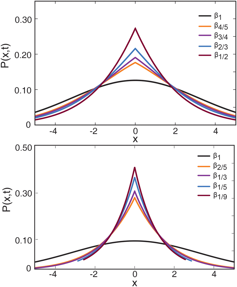 | ||
| Fig. 1 The spreading of particles from a point source into an unbounded one-dimensional space at t = 5 for Brownian and eight distinct anomalous cases with 0 < β < 1. For the Brownian case (β = 1), the black curve shows smooth particle spreading behaviour from the origin. Anomalous diffusion plots show the increase in localisation of particles near the origin in the form of a cusp and the concomitant slower release away from the origin with a decrease in β values. In the plots we set K1 = Kβ = 1. | ||
The deviations of the PDF for β ≠ 1 from classical Brownian motion indicate the need for further investigation into the characteristics of anomalous diffusion. To explore how variations in the value of β influence the localisation of particles near the origin and their subsequent release away from the origin, we performed the subordination integration and derived the PDF across seven distinct β values:  . The shapes of the subordination kernel
 ![[scr E, script letter E]](https://www.rsc.org/images/entities/char_e140.gif) β for the selected β values are reported as eqn (S-1) to (S-7) in the ESI.† The PDFs for these β values were evaluated by performing the subordination integration (5) based on eqn (2) and each of the newly derived
β for the selected β values are reported as eqn (S-1) to (S-7) in the ESI.† The PDFs for these β values were evaluated by performing the subordination integration (5) based on eqn (2) and each of the newly derived  forms. The resulting PDFs from this integration are reported as eqn (A1)–(A8) in the ESI.† These eight representative cases illustrate that the subordination integration can, in principle, yield analytical solutions for any rational β value within the interval 0 < β ≤ 1.
The PDFs for the selected anomalous diffusion cases reported in Fig. 1a and b demonstrate that all anomalous diffusion solutions exhibit a pronounced cusp near the origin. Notably, as the β values decrease, the relative height of the cusp increases, and the spreading away from the origin decreases at the shown intermediate x. For instance, in Fig. 1a, the peak heights and spreading behaviour for the cases  and
and  rather closely resemble (apart from the cusp) the particle spreading observed for the Brownian PDF. In contrast, in Fig. 1b, the peak heights for
  and
and  are significantly higher than the Brownian solution, leading to a more pronounced localisation of the PDF at the origin. Thus, the anomalous diffusion solutions indicate that the decrease in β values results in the release of particles at pronouncedly longer times, leading to particle clustering near the origin. In the next section, we will see how this particle spreading is reflected in the diffusion dynamics through an effectively one-dimensional disordered porous material.
We note that it is also possible to derive the flux solutions from the analytical solutions of the Brownian and anomalous diffusion cases. For the Brownian case, differentiating eqn (2) with respect to x yields the flux
 | (8) |
For anomalous diffusion, the flux solutions for the eight β values are reported in eqn (B1)–(B8) in the ESI.† Note that the diffusion coefficient K1 in eqn (2) is set to 1 during the subordination integration. For β in eqn (7) and eqn. (S-1)–(S-7), κβ is also set to unity. Because both coefficients have generalised length and time units, the resulting PDFs are dimensionless in this non-dimensional choice. The next section revisits the diffusion coefficients to dimensionalise the BTCs to physical time and space units.
3 Results and discussion
3.1 Breakthrough curves and flux
In 1855, Fick combined the continuity equation with a constitutive equation (Fick's first law), according to which the flux is proportional to the chemical gradient and the mass transport of solute species occurs from higher to lower concentration regions. This produces the diffusion equation (Fick's second law) for the chemical concentration field C(x,t),40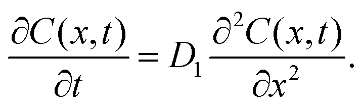 | (9) |
Experimental campaigns typically study solute diffusion, effectively (macroscopically) one-dimensional, from a constant-concentration inlet source through a porous material.18,47–50 The resulting datasets are often presented as BTCs that illustrate the temporal change in relative concentration C(x,t)/C0 measured at the point x away from the inlet source of the sample. For these specific boundary conditions, the analytical solution to eqn (9) reads
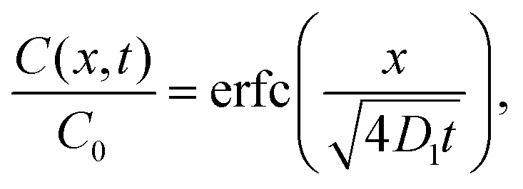 | (10) |
The subordination integration method based on relation (5) and explained in Section 2 can be repeated to obtain the BTCs for the anomalous diffusion case under constant-concentration inlet and semi-infinite boundary conditions, corresponding to subordinating the Fickian expression (10) with  for different β. Metzler et al. (2022)32 reported the BTC for the analytically tractable case of
  , for which the result in eqn (7) is used. Consequently, the resulting BTC illustrates concentration spreading from a constant-concentration inlet source through effectively one-dimensional porous material under the influence of anomalous diffusion. The study utilised the NIntegrate command in Mathematica to perform the subordination integral. The resulting BTCs for both the Fickian case and the anomalous case with
  (along with other β values) are presented in Fig. 2. It is important to note that the value of the diffusivity D1 in eqn (10) was set to 1 cm2 d−1 when performing the subordination integral. Similarly, the anomalous scaling coefficient κ1/2 in eqn (7) was set to 1 d1/2. These coefficients dimensionalise the resulting breakthrough curves into physical space and time units of centimetres and days, respectively. Throughout Section 3.1, the normal diffusion coefficient and anomalous anomalous scaling coefficients are set equal to 1 in the corresponding units while deriving the BTCs using the subordination integration for different β values. They are converted to their specific dimensional values in the following section when adjusted to experimental data.
 | ||
Fig. 2 Normalised BTCs (a and b) and residual BTCs (c and d) for both the Fickian and anomalous models. These solutions are based on diffusion through a 1 cm thick, porous material, i.e., x = 1 in our units. The linear plots illustrate that a decrease in the β value results in a sharper initial arrival of solute species compared to the Fickian case. The residual plots demonstrate that the long-time tails for the Fickian model decay strictly with a slope of  . Conversely, the long-time tails for . Conversely, the long-time tails for  decay with slopes of decay with slopes of  , respectively. , respectively. | ||
Fig. 2 illustrates the normalised BTCs for Fickian diffusion and anomalous diffusion with β ≠ 1. The BTCs Cβ(x,t)/C0 are plotted on linear scales, while the residual BTCs (1 −Cβ(x,t)/C0) are depicted on log10–log10 scale, to highlight the power-law asymptote. The two top panels (a and b) in this figure depict the BTCs and the two bottom panels (c and d) depict the residual BTCs. Let us first discuss the particular cases β = 1 versus . Fig. 2a shows that the BTC for anomalous diffusion with
  has a steeper initial increase in C/C0 than Fickian diffusion. The long-time diffusion behaviour can be assessed by examining the tails36
| 1 − Cβ(x,t)/C0 ∼ x/[Γ(1 − β/2)tβ/2] | (11) |
 . Utilising the relationship β = 2|slope| we find that β = 1 for Fickian diffusion, as it should be. Fig. 2c also presents the residual BTC for anomalous diffusion for the case
  . Notably, the slope of the long-time tail for this residual BTC is
  , which is strictly less than the value
  observed in the Fickian diffusion case. Thus, it can be concluded that anomalous diffusion results in a slower release of solutes over time compared to Fickian diffusion, as expected. Throughout the ensuing discussion and data presentation, the sharp increase of C/C0 at initial time intervals in the BTCs and the slope of the tails of the residual BTCs will be referred to as initial arrival times and long-time tailing, respectively.
The numerical subordination integration approach introduced by Metzler et al. (2022)32 for the specific case  can be extended to scenarios when β is a rational number, and the time kernel then can be shown to consist of, e.g., simple exponential, Airy, or lower-order Fox H-functions. In that study, kernels for
  were constructed using these relatively simple functions. The BTCs and the residual BTCs for the three anomalous diffusion cases were obtained by performing the subordination integration between the time kernel of each β value (eqn (S-2), (S-3), and (S-5)) and the solution to Fickian diffusion (eqn (10)). Fig. 2 we show the BTCs and residual BTCs for these and several other β values along with the Fickian case. As can be seen in panels (a) and (b) of Fig. 2 the linear BTCs increasingly deviate from the Fickian case β = 1 for decreasing β values, with steeper behaviour at short times and slower increase of Cβ(x,t)/C0 at longer times. We note that any real-valued β can be well approximated by a rational number.
The residual BTCs depicted in panels (c) and (d) of Fig. 2 show the crossover from the initial value 1 − Cβ(x,0)/C0 = 1 to the long time inverse power-law behaviour 1 − Cβ(x,t)/C0 ∼ x/[Γ(1 − β/2)tβ/2]. For instance, for anomalous diffusion with  the slopes of the long-time tails are
  , respectively. These slopes indicate that a decrease in the value of β results in a slower release of solutes from the outlet sample boundary in anomalous diffusion, relative to Fickian diffusion. The experimental data presented below in Fig. 4 clearly demonstrate a relevant power-law behaviour with β ≠ 1 supporting the CTRW approach.
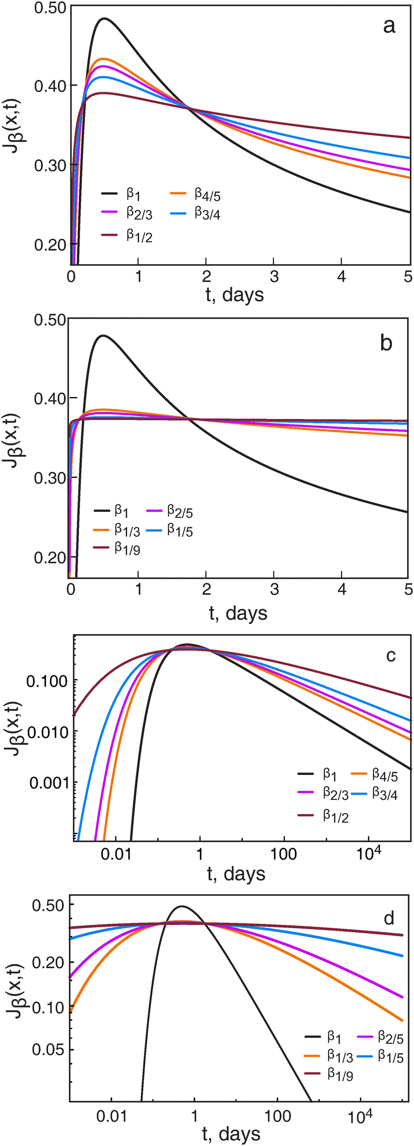 | ||
Fig. 3 The flux J(x,t) vs. t (a and b) and log10(J(x,t)) vs. log10(t) (c and d) for both Fickian and anomalous models. These plots represent the solutes crossing the point x = 1 cm of a semi-infinite porous material. The linear plots illustrate that a decrease in the β value results in a sharper initial flux rise compared to the more gradual rise in the Fickian case. The log–log plots demonstrate that the decrease in β values causes a slight decrease in the maximum flux compared to the Fickian model. Once the maximum flux is attained, the long-time tails of the Fickian model strictly decay with the slope  , while the long-time tails for β ≠ 1 corresponds to −β/2. , while the long-time tails for β ≠ 1 corresponds to −β/2. | ||
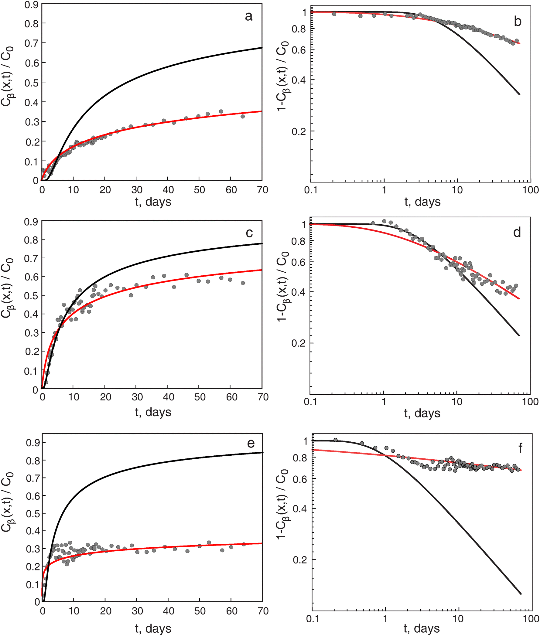 | ||
Fig. 4 Fickian (black line) and anomalous (red line) solutions represented as (left panels) BTCs and (right panels) residual BTCs. The numerical BTCs/residual BTCs are plotted against the experimental data (black points) obtained from bromide diffusion experiments31 through three porous rock samples. The red lines correspond to (a and b)  for DP, (c and d) for DP, (c and d)  for EY, and (e and f) for EY, and (e and f)  for SL, respectively. The solutions are calculated for solute diffusion through an effectively one-dimensional, semi-infinite porous medium with sampling point x = 1 cm. The residual BTCs show that the long-time tails of anomalous diffusion always decay with a slope shallower than for SL, respectively. The solutions are calculated for solute diffusion through an effectively one-dimensional, semi-infinite porous medium with sampling point x = 1 cm. The residual BTCs show that the long-time tails of anomalous diffusion always decay with a slope shallower than  (the slope for the Fickian case). The measured data interpolate between a short-time Fickian behaviour and clear anomalous diffusion with β ≠ 1 are intermediate- to long-times. (the slope for the Fickian case). The measured data interpolate between a short-time Fickian behaviour and clear anomalous diffusion with β ≠ 1 are intermediate- to long-times. | ||
On a more technical note, for the cases  , the calculation of BTCs using the NIntegrate method between eqn (10) and each of eqn (S-1), (S-4), (S-6), and (S-7) is limited by oscillating terms in the higher-order H-functions. To resolve this issue, we incorporated a “stability term” μ(s,t) with an exponential decay into the subordination integral in the form
  , to enforce the convergence. The exact form of the individual stability terms for
  are detailed in the ESI† along with numerical proof that this trick does not significantly change the behaviour of the resulting BTCs in the relevant time window. As shown in Fig. 2 the results for these smaller β values for both the linear BTCs and the residual BTCs continue the discussed trends away from the Fickian case for decreasing β.
Alternatively, the datasets can be represented in terms of the flux J(x,t), describing the number of particles crossing the point x as function of time.52–54 The flux for Fickian diffusion can be evaluated by differentiating eqn (10) with respect to x, yielding
 | (12) |
β. At long times the flux has the inverse power-law behaviour Jβ(x,t) ∼ C0/[Γ(1 − β/2)tβ/2].32 The resulting flux curves for various β are displayed in Fig. 3.
The rapid increase in flux suggests that pore solution equilibration with the solutes due to anomalous diffusion occurs more rapidly than for the Fickian case. The long time shapes also indicate that solutes with anomalous diffusion are released at slower rates over extended periods than those for Fickian diffusion. Thus, these differences can result in variations in the initial spreading of solutes, mean residence and trapping times of solutes in pore spaces, and the long-term release of solutes from the porous material.
3.2 Modelling diffusion experiments
The BTCs and flux solutions can be dimensionalised to experimental conditions to quantify experimental diffusion results. This section will examine the datasets from a recent experimental study conducted by Rajyaguru et al. in 2024,31 which investigated the diffusion of bromide through porous rock samples composed of chalk and dolomite. We focus on three specific experimental datasets from this research: Desert Pink PL, Edwards Yellow PL, and Silurian Dolomite PL, referred to as DP, EY, and SL, respectively. These diffusion datasets were obtained under a constant concentration at the inlet and a semi-infinite outlet boundary and reported in Fig. 4, respectively. The associated β values for the long-time tails were estimated from the residual BTCs using the relationship β = 2 × |slope|. Table 1 presents these experimental β values, which are clearly less than the Fickian diffusion exponent of 1. Furthermore, the experimental datasets presented in Rajyaguru et al. (2024)31 were compared with asymptotic curves derived under the Fickian case, using the relationship , and for the anomalous case, represented by
  . By optimising the standard diffusion coefficient (D1, in cm2 d−1) in the Fickian case and the anomalous diffusion coefficient (Dβ, in cm2 d−β) in the anomalous case, these asymptotic solutions were tailored to align with the experimental conditions. Rajyaguru et al. (2024)31 found notable correlations between the asymptotic anomalous plots and the long-time tails observed in the experimental data. As a result, the study concluded that the long-time concentration tails exhibited anomalous behaviour.
| β | κ β (d1−β) | D 1 (cm2 d−1) | |
|---|---|---|---|
| Desert Pink | 0.26 | 0.65 | 0.105 |
| Edwards Yellow | 0.49 | 0.60 | 0.225 |
| Silurian Dolomite | 0.08 | 1.5 | 0.285 |
In an initial effort to quantify the results, the Fickian diffusion-based BTCs were plotted against experimental datasets, as shown in Fig. 4. These BTCs were derived by dimensionalising eqn (10) with normal diffusion coefficients of 0.04 for DP, 0.09 for EY, and 0.17 for SL. These values were chosen as they generally represent anionic diffusion into carbonate rocks.47,55,56Fig. 4 demonstrates that the dimensionalised BTCs effectively model the experimental datasets for all three samples during the initial 4, 8, and 10 days. However, as the long-time tails of Fickian diffusion decay with a slope of  , notable divergences are visible between the long-time experimental and numerical BTCs. Thus, to comprehensively quantify the experimental BTCs for the three rock samples, it is necessary to dimensionalise the anomalous BTCs from Section 2 to integrate the characteristics of early-time Fickian and intermediate-to-long-time anomalous diffusion behaviour.
The experimental datasets presented in Fig. 4 were quantified using the solutions for β values of  for DP,
  for EY, and
  for SL. In the initial step, the optimised normal diffusion coefficients detailed in Table 1 were employed to dimensionalise the Fickian diffusion solution (10) to the experimental conditions. Next, the optimised anomalous scaling coefficient κβ values from Table 1 were inserted in each of the corresponding time kernels to dimensionalise them with the experimental conditions. Finally, we performed the subordination integration between the dimensionalised Fickian diffusion eqn (10) and the corresponding time kernels (7) for DP, (S-3, ESI†) for EY, and (S-6, ESI†) for SL to derive the BTCs. The resulting BTCs for each case are plotted in Fig. 4. Interestingly, the normal diffusion coefficient values used for dimensionalising the Fickian part in the subordination integration differs from those used for dimensionalising the full Fickian diffusion-based BTCs in Fig. 4. The Fickian contribution is relevant only at short times, before the solute explores the environment fully and immobilisation effects described by ψ(τ), and therefore anomalous diffusion, become dominant.
Fig. 4a–f shows the BTCs and residual BTCs for experiments, plotted against the corresponding dimensionalised curves for anomalous and Fickian diffusion. Fig. 4 shows that the three distinct anomalous diffusion exponents match the data for the BTCs/residual BTCs for the three rock samples. Specifically, the BTCs and residual BTCs in Fig. 4a and b show that the scaled solution of  matches the experimental datasets for the DP sample at intermediate-to-longer times. Fig. 4c–f analogously demonstrates that the scaled solutions for
  and
and  match the intermediate-to-longer time behaviour of the EY and SL experiments. Furthermore, Fig. 4 shows that the experimental dataset for each rock sample interpolates between the early-time Fickian and intermediate to long-time anomalous diffusion regimes. As mentioned earlier, for each case, the scaled Fickian BTCs can effectively model the experimental data points during the initial 4, 8, and 10 days, respectively. This shows that when data are sampled only at relatively short times after solute release, the measured behaviour becomes indistinguishable from Fickian behaviour. This initial behaviour can be physically explained as follows: at early times, when the first solute arrive in the sample, they are typically all mobile until an increasing amount of the particles are eventually trapped. This observation indicates that the immobilisation process in the CTRW model is clearly exhibited only after some time. Thus, long-term diffusion dynamics are increasingly dominated by the trapping effects of solutes in the rock pore spaces. As the rock samples have distinct pore structure heterogeneity, they can induce distinct trapping dynamics and, thereby, distinct emergence of the long-time tails. Indeed, the consistent emergence of the long-time tails in the experimental datasets for three rock samples confirms these observations.
To better illustrate the contrasting effects of anomalous and Fickian diffusion on solutes spreading and their release over time, we developed flux solutions tailored to the three different rock sample conditions. The flux solutions accounting for pure Fickian diffusion were dimensionalised using the same normal diffusion coefficient values (D1 values equal to 0.04 for DP, 0.09 for EY, and 0.17 for SL (cm2 d−1)) used to dimensionalise the Fickian BTCs reported in Fig. 4. These diffusion coefficient values were inserted in eqn (12) and the resulting linear and residual flux solutions are shown in Fig. 5. The anomalous diffusion flux solutions were derived using the previously explained NIntegrate method for deriving the BTCs dimensionalised to experimental conditions. In the NIntegrate method, the dimensionalised eqn (10) was replaced with eqn (12). The resulting linear and residual anomalous flux solutions are reported against flux solutions in Fig. 5a, c, and e, for three samples, DP, EY, and SL, respectively. During the initial, early-time phase of the experiments, the (anomalous diffusion) solutions show a flux increase like the Fickian flux solution. This observation is consistent with the linear experimental BTCs depicted in Fig. 4a, c, and d, where bromide diffusion appears to follow Fickian diffusion for the first 10, 8, and 4 days in DP, EY, and SL, respectively. The solution plots in Fig. 5b, d, and f indicate that the maximum flux points for the anomalous cases are lower than those for the Fickian cases. These observations align with the experimental findings that demonstrate a lower Cβ(x,t)/C0 point after which long-time tails emerge, and the rate at which Cβ(x,t)/C0 increases at the sample boundary is slower than Fickian modelling. For instance, the Cβ(x,t)/C0 for DP is 0.16 at 10 days, after which the long-time tails emerge. At this point, the Cβ(x,t)/C0 for the scaled Fickian solution is 0.49. Table 1 shows that the β value of the long-time tails for the DP experiment is 0.26 compared to 0.92 for the scaled Fickian model.
 | ||
Fig. 5 Flux as function of time corresponding to the BTC/residual BTC data shown in Fig. 4. Black curves show the pure Fickian case while red curves correspond to the pure anomalous diffusion case. Flux J(x,t) vs. t (a, c and e) and log10(J(x,t)) vs. log10(t) (b, d and f). The flux is shown (left) on linear scales and (right) in a log10–log10 plot. The anomalous diffusion exponents are (a and b)  , (c and d) , (c and d)  , and (e and f) , and (e and f)  . The solutions are calculated for solute diffusion through an effectively one-dimensional porous medium with sampling point at x = 1 cm. The long-time tails have slope . The solutions are calculated for solute diffusion through an effectively one-dimensional porous medium with sampling point at x = 1 cm. The long-time tails have slope  for the Fickian case and for the Fickian case and  for the anomalous diffusion cases. for the anomalous diffusion cases. | ||
3.3 Implications of anomalous diffusion in natural systems
Laboratory-scale experiments are conducted in geosciences to elucidate the impact of porous material properties on solute mass transport under various controlled conditions (e.g., pH, ionic strength, type of solute).47 For diffusion studies, laboratory-scale experiments play an important role, for instance, in estimating radionuclide diffusion through clay-rich lithologies and solute transport mechanisms in carbonate environments.12,55–59 Such studies are pivotal for designing and assessing deep geological repositories, e.g., leveraging claystone as a natural containment barrier,60 and for evaluating the spreading of solutes into coastal or inland aquifers and through river, lake and marine sediments.To underscore the significance of anomalous diffusion in natural systems, we illustrate the normalised concentration profiles Cβ(x,t)/C0 based on pure Fickian and pure anomalous diffusion at different times in Fig. 6. These solutions were generated using the dimensionalised subordination approach outlined in Section 3.2 to derive BTCs for the DP  , EY
, EY  , and SL
  rock samples under conditions of anomalous and Fickian diffusion. Fig. 6 shows the dimensionalised profiles for Fickian and anomalous diffusion at five different times for bromide solute diffusion through a 100 cm thick rock formation. Here, the profiles for Fickian diffusion indicate that after 10
![[thin space (1/6-em)]](https://www.rsc.org/images/entities/char_2009.gif) 000 days, the solute penetrates 80 cm of the DP rock formation and 100 cm of the EY and SL layers. Conversely, the profiles for anomalous diffusion for the three rock samples are significantly different even at relatively early times (100 d). After 10000 days, anomalous diffusion allows bromide penetration of only 20 cm, 40 cm, and 10 cm in the DP, EY, and SL rocks, respectively. Clearly, the solutions shown here demonstrate that the times and distances relevant for initial solute arrival, and for diffusive leaching of solutes from contaminated rock formations, are significantly longer than under the assumption of Fickian diffusion.
000 days, the solute penetrates 80 cm of the DP rock formation and 100 cm of the EY and SL layers. Conversely, the profiles for anomalous diffusion for the three rock samples are significantly different even at relatively early times (100 d). After 10000 days, anomalous diffusion allows bromide penetration of only 20 cm, 40 cm, and 10 cm in the DP, EY, and SL rocks, respectively. Clearly, the solutions shown here demonstrate that the times and distances relevant for initial solute arrival, and for diffusive leaching of solutes from contaminated rock formations, are significantly longer than under the assumption of Fickian diffusion.
 | ||
| Fig. 6 Evolution of the normalised concentration profile Cβ(x,t)/C0 for bromide diffusion within 1 m of rock for 100 d, 500 d, 1000 d, 5000 d, and 10000 d for a semi-infinite rock sample with constant-concentration inlet. The dashed lines correspond to Fickian diffusion, the solid lines represent anomalous diffusion. The plots in sequential order correspond to Desert Pink PL, Edwards Yellow PL, and Silurian Dolomite PL, respectively. | ||
4 Conclusions
We work with the CTRW framework to model the anomalous diffusion of solute species through disordered porous materials. We develop solutions representing the full range of anomalous diffusion, from highly anomalous to Fickian, yielding BTCs and fluxes. The solution method demonstrates that this framework can be applied to derive a solution for any fractional β value within the interval 0 < β < 1. Furthermore, we show that the solutions for various values of β can be dimensionalised to experimental space and time units, by using the normal and anomalous diffusion coefficients derived from the high-resolution datasets.31 Our analysis of experimentally determined BTCs, accounting for anomalous diffusion, reveals that anomalous diffusion may appear indistinguishable from Fickian behaviour within relatively short periods from the start of solute release into a domain. However, at intermediate-to-longer times, anomalous diffusion of solutes leads to significantly different patterns of migration relative to Fickian diffusion.What controls the occurrence of anomalous diffusion in porous systems? A concrete answer depends upon the specific details of the system under consideration, as well as on the measured length and time scales. Several specific mechanisms that affect the observed anomalous diffusion can be identified:37 (i) hindered diffusion (due to the reduced available fraction of space): the authors37 conclude that this is a minor effect in the considered materials; (ii) hydrodynamic coupling effects: the authors37 conclude that this is mainly relevant in the presence of a drift, and therefore not relevant for the current study; (iii) transient binding to the rock matrix: this could be a potential effect for the current system; (iv) pore accessibility: due to the finite size of the tracer, the pore size appears to have a major effect on the pore structures, with constrictions of the order of the size of the tracer. In general, system parameters such as the compaction of the porous materials and physical pore structure heterogeneity, possibly combined with transient binding to the rock matrix, will thus control the crossover from initial Fickian to long-time anomalous diffusion behaviour. At much longer times, as addressed below, a crossover back to Fickian transport is expected to eventually occur (whether measurable within the available experimental window or not).
The occurrence of anomalous diffusion has important implications mainly because it indicates significant differences in the migration of solutes through porous rock structures compared to universally assumed Fickian diffusion models. These differences have a critical impact on both early and late-time arrivals of solutes to a control plane, as well as the average residence time of solute species in porous materials and their overall release rate from these materials.
Apparent anomalous behaviour subject to advection, dispersion, and diffusion was previously studied for the fraction of injected mass from the MADE-1 experiment, first in terms of a general CTRW framework,61 and then in terms of a limit-case “fractal” mobile-immobile model with a fractional time derivative.62,63 Apparent anomalous scaling of the MSD may even arise in mobile-immobile diffusion of particles with Poissonian switching between the mobile and immobile phases, when the mean immobilisation time is significantly longer than the mean mobile time.64 Moreover, clear evidence for anomalous behaviour subject to advective-dispersive-diffusive transport was also discussed in the context of contaminant transport in stream catchments.65,66 Compared to these experiments, the method introduce here focused on pure diffusion of solutes away from a constant-concentration inlet. In this situation there arise distinct inverse power-law shapes of the residual BTCs, from which the anomalous diffusion exponent β can be directly assessed. The measured data in three different rock samples discussed here clearly support the power-law behaviour of the residual BTCs with a single β in a given sample, thus providing unequivocal support for the existence of anomalous diffusion in these samples.
We note that anomalous diffusion-dominated transport was already conclusively revealed for charge carrier motion (“Scher–Montroll transport”) in amorphous and polymeric semiconductors.67,68 In these types of experiments the electrical current can be directly measured, demonstrating that the current has two subsequent power-law regimes whose slopes, β − 1 and −β −1 with 0 < β < 1, add up to −2.67 This behaviour can be understood as a first-passage time process, even in the case of ageing, when the charge carriers are first allowed to get progressively trapped in the semiconductor, before the driving electrical field is switched on.68–70
Finally we note that the anomalous diffusion modelling here based on the long-tailed waiting time PDF ψ(τ) ≃ τ−1−β introduced in the CTRW model. For 0 < β < 1 the mean waiting time 〈τ〉 thus diverges. This model was shown here to provide an appropriate quantitative description of our data. However, at much longer times the waiting time PDF may have a cutoff corresponding to the longest immobilisation time τmax in the system (see Fig. 7). Possible causes for such a tempering of ψ(τ) may be due to the pore structure accessibility being limited by a smallest, finite physical size and/or the existence of a maximal bromide-pore surface binding time. In such cases, a long-time, effectively Fickian behaviour at time t ≫ τmax may be recovered. However, this long-time “normal-diffusive” regime would then be characterised by a significantly smaller value of the effective diffusion coefficient, “dressed” by continuing immobilisation events with waiting times τ < τmax.71
 | ||
| Fig. 7 Schematic illustration of the concentration spreading of solutes relative to their distance x from the sample inlet source. Initially, under highly dilute conditions, solute diffusion follows the principles of normal diffusion. As more particles become present in the sample pore solution, an immobilisation effect emerges, leading to intermediate to long-timescale anomalous diffusion. In a physical system, after extended time scales, the subdiffusive growth typically culminates in a second crossover point, at which solute spreading resumes a linear pattern with a reduced diffusion constant (D < D1) or reaches saturation. | ||
Given the potential implications of such behaviour in geological, biological, and engineering settings, the observed deviations between Fickian and anomalous diffusion models underscore the need to reassess estimates of chemical diffusion rates and patterns in systems where Fickian diffusion has been universally assumed. In the future more elaborate diffusion and transport models should be developed that combine early-stage Fickian and intermediate- to long-time anomalous motion, possibly with a “truncated” waiting time PDF cutting off the power-law of the immobilisations. Moreover, improved experiments of the type presented here for longer times and different rock samples are desirable.
Data availability
The manuscript and the ESI† provide ancillary calculations, equations, and solutions used in this publication. The experimental datasets used in this publication are available from the previous publication: “Rajyaguru et al. 2024,31 Diffusion in porous material is anomalous. DOI: https://pubs.acs.org/doi/10.1021/acs.est.4c01386.Conflicts of interest
All authors agreed to the material in this manuscript and share no conflict of interest.Acknowledgements
A. R. was partly supported by the European Union's Horizon 2020 research program under the Marie Sklodowska-Curie grant agreement no. 701647 and partly by the Swiss Society of Friends of the Weizmann Institute of Science. R. M. acknowledges support from the German Research Foundation (DFG, grant ME 1535/12-1). B. B. was supported by the ViTamins project, funded by the Volkswagen Foundation (grant no. AZ 9B192), and by a research grant from the Crystal Family Foundation, Mr Stephen Gross, the Emerald Foundation, the P. & A. Guggenheim-Ascarelli Foundation, and the DeWoskin/Roskin Foundation. B. B. holds the Sam Zuckerberg Professorial Chair in Hydrology.Notes and references
- J. W. Kirchner, X. Feng and C. Neal, Nature, 2000, 403, 524–527 CrossRef CAS PubMed.
- K. L. Blann, J. L. Anderson, G. R. Sands and B. Vondracek, Crit. Rev. Environ. Sci. Technol., 2009, 39, 909–1001 CrossRef CAS.
- N. Benoit, A. Dove, D. Burniston and D. Boyd, J. Environ. Prot., 2016, 7, 390–409 CrossRef CAS.
- N. Goeppert, N. Goldscheider and B. Berkowitz, Water Res., 2020, 178, 115755 CrossRef CAS PubMed.
- E. Zehe, R. Loritz, Y. Edery and B. Berkowitz, Hydrol. Earth Sys. Sci., 2021, 25, 5337–5353 CrossRef CAS.
- A. Izadpanahi, M. J. Blunt, N. Kumar, M. Ali, C. C. G. Tassinari and M. A. Sampaio, Fuel, 2024, 369, 131744 CrossRef CAS.
- V. Briane, M. Vimond and C. Kervrann, Brief. Bioinf., 2020, 21, 1136–1150 CrossRef CAS PubMed.
- M. Rolle, M. Albrecht and R. Sprocati, J. Contam. Hydrol., 2022, 244, 103933 CrossRef CAS PubMed.
- D.-X. Guan, S.-X. He, G. Li, H. H. Teng and Q. M. Lena, Crit. Rev. Environ. Sci. Technol., 2022, 52, 3035–3079 CrossRef CAS.
- F. N. Cayan, S. R. Pakalapati, F. Elizalde-Blancas and I. Celik, J. Power Sources, 2009, 192, 467–474 CrossRef CAS.
- J. Yuan and B. Sundén, Int. J. Heat Mass Transfer, 2014, 69, 358–374 CrossRef.
- S. Altmann, M. Aertsens, T. Appelo, C. Bruggeman, S. Gaboreau, M. Glaus, P. Jacquier, T. Kupcik, N. Maes, T. R. V. Montoya, J. Robinet, S. Savoye, T. Schaefer, C. Tournassat, L. V. Laer and L. V. Loon, Processes of cation migration in clayrocks: Final Scientific Report of the CatClay European Project, 2015 Search PubMed.
- C. I. Steefel and M. Hu, Water Resour. Res., 2022, 58, e2022WR032321 CrossRef CAS.
- A. Jonathan, E. M. Moon, K. G. Schulz and A. L. Rose, J. Phys. Chem. Lett., 2023, 14, 4517–4523 CrossRef PubMed.
- L. Sessegolo, A. Verney-Carron, M. Saheb, L. Remusat, A. Gonzalez-Cano, N. Nuns, J.-D. Mertz, C. Loisel and A. Chabas, NPJ Mater. Degrad., 2018, 2, 17 CrossRef.
- Z. Bo, M. Boon, H. Hajibeygi and S. Hurter, Int. J. Hydrogen Energy, 2023, 48, 13527–13542 CrossRef CAS.
- V. Arekhov, T. Clemens, J. Wegne, M. Abdelmoula and T. Manai, SPE Reservoir Eval. Eng., 2023, 26, 1566–1582 CrossRef.
- A. Rajyaguru, N. Seigneur, O. Bildstein, S. Savoye, C. Wittebroodt, E. L'Hôpital, V. Detilleux, P. Arnoux and V. Lagneau, Chem. Geol., 2022, 609, 121069 CrossRef CAS.
- R. Metzler, J.-H. Jeon, A. G. Cherstvy and E. Barkai, Phys. Chem. Chem. Phys., 2014, 16, 24128–24164 RSC.
- I. Golding and E. C. Cox, Phys. Rev. Lett., 2006, 96, 098102 CrossRef PubMed.
- C. Nicholson, Biophys. J., 2015, 108, 2091–2093 CrossRef CAS PubMed.
- W. He, H. Song, Y. Su, L. Geng, B. J. Ackerson, H. Peng and P. Tong, Nat. Commun., 2016, 7, 11701 CrossRef CAS PubMed.
- J.-H. Jeon, M. Javanainen, H. Martinez-Seara, R. Metzler and I. Vattulainen, Phys. Rev. X, 2016, 6, 021006 Search PubMed.
- J.-H. Jeon, N. Leijnse, L. B. Oddershede and R. Metzler, New J. Phys., 2013, 15, 045011 CrossRef CAS.
- A. D. Fernández, P. Charchar, A. G. Cherstvy, R. Metzler and M. W. Finnis, Phys. Chem. Chem. Phys., 2020, 22, 27955–27965 RSC.
- S. Trillot, N. Tarrat, N. Combe, P. Benzo, C. Bonafos and M. Benoit, J. Chem. Phys., 2025, 162, 104701 CrossRef CAS PubMed.
- C. Bousige, P. Levitz and B. Coasne, Nat. Commun., 2021, 12, 1043 CrossRef CAS PubMed.
- S. Havlin and D. Ben-Avraham, Adv. Phys., 1987, 36, 695–798 CrossRef CAS.
- J. Feder, Fractals, Plenum Press, New York, NY, 1989 Search PubMed.
- A. Klemm, R. Metzler and R. Kimmich, Phys. Rev. E, 2002, 65, 021112 CrossRef PubMed.
- A. Rajyaguru, R. Metzler, I. Dror, D. Grolimund and B. Berkowitz, Environ. Sci. Technol., 2024, 58, 8946–8954 CrossRef CAS PubMed.
- R. Metzler, A. Rajyaguru and B. Berkowitz, New J. Phys., 2022, 24, 123004 CrossRef.
- R. Brown, Ann. Phys., 1828, 90, 294–313 CrossRef.
- A. Einstein, Investigations on the Theory of the Brownian Movement, Dover Publications, Inc., New York, NY, 1956 Search PubMed.
- M. von Smoluchowski, Ann. Phys., 1906, 326, 756–780 CrossRef.
- R. Metzler and J. Klafter, Phys. Rep., 2000, 339, 1–77 CrossRef CAS.
- H. Wu and D. K. Schwartz, Acc. Chem. Res., 2020, 53, 2130–2139 Search PubMed.
- M. Magdziarz, A. Weron and J. Klafter, Phys. Rev. Lett., 2008, 101, 210601 CrossRef PubMed.
- S. Bochner, Proc. Natl. Acad. Sci. U. S. A., 1962, 48, 2039–2043 CrossRef CAS PubMed.
- A. Fick, Ann. Phys., 1855, 170, 59–86 Search PubMed.
- B. D. Hughes, Random walks and random environments, Oxford University Press, 1995, vol. 1, Random Walks Search PubMed.
- L. Yuan-Hui and S. Gregory, Geochim. Cosmochim. Acta, 1974, 38, 703–714 CrossRef.
- B. Jin, M. Rolle, T. Li and S. B. Haderlein, Environ. Sci. Technol., 2014, 48, 6141–6150 Search PubMed.
- K. Longnecker and E. B. Kujawinski, Geochim. Cosmochim. Acta, 2011, 75, 2752–2761 CrossRef CAS.
- M. Rolle, G. Chiogna, D. L. Hochstetler and P. K. Kitanidis, J. Contam. Hydrol., 2013, 153, 51–68 CrossRef CAS PubMed.
- M. Rolle and B. Jin, Environ. Sci. Technol., 2017, 4, 298–304 CAS.
- A. Rajyaguru, E. L'Hôpital, S. Savoye, C. Wittebroodt, O. Bildstein, P. Arnoux, V. Detilleux, I. Fatnassi, P. Gouze and V. Lagneau, Chem. Geol., 2019, 503, 29–39 CrossRef CAS.
- S. Didierjean, D. Maillet and C. Moyne, Adv. Water Res., 2004, 27, 657–667 CrossRef.
- G. J. Moridis, Water Resour. Res., 1999, 35, 1729–1740 CrossRef.
- L. R. V. Loon and J. Mibus, Appl. Geochem., 2015, 59, 85–94 CrossRef.
- M. Abramowitz and I. A. Stegun, Handbook of mathematical functions, Dover Publications, Inc., New York, NY, 1972 Search PubMed.
- C. Tournassat, C. I. Steefel, P. M. Fox and R. M. Tinnacher, Sci. Rep., 2023, 13, 15029 CrossRef CAS PubMed.
- P. M. Fox, C. Tournassat, C. I. Steefel and P. S. Nico, Appl. Geochem., 2024, 170, 106090 CrossRef CAS.
- E. Tertre, S. Savoye, F. Hubert, D. Prêt, T. Dabat and E. Ferrage, Environ. Sci. Technol., 2018, 52, 1899–1907 CrossRef CAS PubMed.
- M. Descostes, V. Virginie Blin, F. Bazer-Bachi, P. Meier, B. Grenut, J. Radwan, M. L. Schlegel, S. Buschaert, D. Coelho and E. Tevissen, Appl. Geochem., 2008, 23, 655–677 CrossRef CAS.
- M. Descostes, E. Pili, O. Felix, B. Frasca, J. Radwan and A. Juery, J. Hydrol., 2012, 452, 40–50 CrossRef.
- L. R. V. Loon, P. Bunic, S. Frick, M. A. Glaus and R. A. Wüst, Appl. Geochem., 2023, 159, 105843 CrossRef.
- S. Savoye, C. Beaucaire, B. Grenut and A. Fayette, Appl. Geochem., 2015, 61, 41–52 CrossRef CAS.
- E. Tertre, A. Delville, D. Prêt, F. Hubert and E. Ferrage, Geochim. Cosmochim. Acta, 2015, 149, 251–267 CrossRef CAS.
- M. Mazurek, T. Gimmi, C. Zwahlen, L. Aschwanden, E. C. Gaucher, M. Kiczka, D. Rufer, P. Wersin, M. M. Fernandes and M. A. Glaus, et al. , Appl. Geochem., 2023, 159, 105839 CrossRef CAS.
- B. Berkowitz and H. Scher, Phys. Rev. E, 1998, 57, 5858 CrossRef CAS.
- R. Schumer, D. A. Benson, M. M. Meerschaert and B. Baeumer, Water Resour. Res., 2003, 39, 13 Search PubMed.
- T. J. Doerries, A. V. Chechkin, R. Schumer and R. Metzler, Phys. Rev. E, 2022, 105, 014105 CrossRef CAS PubMed.
- T. J. Doerries, A. V. Chechkin and R. Metzler, J. R. Soc., Interface, 2022, 19, 20220233 CrossRef CAS PubMed.
- J. W. Kirchner, X. Feng and C. Neal, Nature, 2000, 403, 524–527 CrossRef CAS PubMed.
- H. Scher, G. Margolin, R. Metzler, J. Klafter and B. Berkowitz, Geophys. Res. Lett., 2002, 29, 5-1–5-4 CrossRef.
- H. Scher and E. W. Montroll, Phys. Rev. B, 1975, 12, 2455–2477 CrossRef CAS.
- M. Schubert, E. Preis, J. C. Blakesley, P. Pingel, U. Scherf and D. Neher, Phys. Rev. B, 2013, 87, 024203 CrossRef.
- H. Krüsemann, A. Godec and R. Metzler, Phys. Rev. E, 2014, 89, 040101(R) CrossRef PubMed.
- H. Krüsemann, R. Schwarzl and R. Metzler, Transp. Porous Media, 2016, 115, 327–344 CrossRef.
- F. Höfling and T. Franosch, Rep. Prog. Phys., 2013, 76, 046602 CrossRef PubMed.
Footnotes |
| † Electronic supplementary information (ESI) available. See DOI: https://doi.org/10.1039/d5cp00654f |
| ‡ We use ≃ to describe the long-time behaviour ignoring proportionality constants, while ∼ denotes asymptotic equality. |
| § In the CTRW picture s corresponds to the number of jumps, and the subordination method introduces the long-tailed immobilisation times.38 |
¶ Lab-scale diffusion experiments are typically conducted through centimetre scale samples and the BTCs are obtained in time scales of days. Therefore, the unit of  is typically used for the resulting mass diffusion coefficient. is typically used for the resulting mass diffusion coefficient. |
| This journal is © the Owner Societies 2025 |