
 Open Access Article
 This Open Access Article is licensed under a
 Creative Commons Attribution 3.0 Unported Licence
Quantification of vehicular versus uncorrelated Li+–solvent transport in highly concentrated electrolytes via solvent-related Onsager coefficients†
Hendrik
Kilian‡
a,
Tabita
Pothmann‡
a,
Martin
Lorenz
b,
Maleen
Middendorf
bc,
Stefan
Seus
a,
Monika
Schönhoff
 *b and
Bernhard
Roling
*a
*b and
Bernhard
Roling
*a
aDepartment of Chemistry and Center for Materials Science (WZMW), University of Marburg, Hans-Meerwein-Straße 4, 35032 Marburg, Germany. E-mail: roling@staff.uni-marburg.de
bInstitute of Physical Chemistry, University of Münster, Corrensstraße 30, D-48149 Münster, Germany
cInternational Graduate School for Battery Chemistry, Characterization, Analysis, Recycling and Application (BACCARA), University of Münster, Münster, 48149, Germany
First published on 23rd December 2024
Abstract
Highly concentrated salt solutions are promising electrolytes for battery applications due to their low flammability, their high thermal stability, and their good compatibility with electrode materials. Understanding transport processes in highly concentrated electrolytes is a challenging task, since strong ion–ion and ion–solvent interactions lead to highly correlated movements on the microscopic scale. Here, we use an experimental overdetermination method to obtain accurate Onsager transport coefficients for concentrated binary electrolytes composed of either sulfolane (SL) or dimethyl carbonate (DMC) as solvent and either LiTFSI or LiFSI as salt. NMR-based electrophoretic mobilities demonstrate that volume conservation applies as a governing constraint for the transport. This fact allows to calculate the Onsager coefficients σ+0, σ−0 and σ00 related to the solvent. A parameter γ is then defined, which is a measure for the relevance of a vehicular Li+–solvent transport mechanism. We analyze the influence of the salt anion and of the solvent on dynamic correlations and transport mechanisms. In the case of the sulfolane-based electrolytes, the γ parameter reaches values up to 0.38, indicating that Li+–sulfolane interactions are stronger than Li+–anion interactions and that vehicular Li+–sulfolane transport plays a significant role. In the case of DMC-based electrolytes, the γ parameter is close to zero, suggesting balanced Li+–DMC vs. Li+–anion interactions and virtually uncorrelated movements of Li+ ions and DMC molecules.
Introduction
The conventional lithium-ion battery (LIB) uses a mixture of organic carbonates in combination with LiPF6 as its electrolyte, where the carbonate oxygens are stabilizing the Li+ ions by coordination of their electron-donating oxygens.1,2 To ensure high ionic conductivity and fast lithium-ion transport, this electrolyte has a rather low salt concentration of 1 mol L−1 and therefore an excess of solvent molecules.3 Consequently, the electrolyte exhibits a considerable safety risk due to the free organic carbonate molecules and their high vapor pressure and low flash point.4–7 Additionally, the electrochemical stability of the solvent molecules and the electrolyte as a whole is limited. The range of reduction potentials of typically used electrode materials, like graphite as an anode and lithium cobalt oxide (LCO) or lithium nickel manganese cobalt oxide (NMC) as cathode, ranges from about 0.1 V up to about 4 V vs. Li/Li+.8,9 The electrolyte, however, has a smaller electrochemical stability window so that degradation of its components at the electrodes occurs, which limits long-term stability and lifetime of the battery.2 This also prevents usage of high-voltage cathode materials, like LiNi0.5Mn1.5O4.10,11 Therefore, the development of an electrolyte that not only exhibits a higher thermal stability, but also has a broader electrochemical stability window is crucial for future generations of lithium-ion batteries.One alternative electrolyte class are highly concentrated electrolytes (HCE), which have a much higher salt concentration than conventional electrolytes in the range of 5 to 6 M.3 While in a 1 M electrolyte, the Li+ ions are typically coordinated by 4–5 solvent molecules, this type of coordination is not possible in HCEs. Thus, the molecular structure of HCEs differs drastically from that of more dilute electrolytes.3,12,13 This includes structures like contact ion pairs (CIP) and aggregates (AGG), where anions are also involved in the solvation of lithium ions and different donor molecules are shared by multiple cations.12,14 These aggregates become more complex at increasing salt concentrations due to the overlap of the solvation shells of the lithium ions.12 Since virtually all solvent molecules are coordinated to Li+ ions, the properties of the solvent molecules change drastically, which causes the vapor pressure of the electrolyte to decrease and the electrochemical and thermal stability of the electrolyte to increase. The HCEs are therefore hardly or not flammable at all, resulting in a reduced safety risk.3,12 On the other hand, the viscosity of the electrolyte rises sharply and each movement of an ion is highly influenced by its surrounding ions and solvent molecules and their mutual interactions.15,16 Understanding these correlated movements is a key factor when investigating HCEs in order to optimize charge and mass transport.17–21
Commonly salts, like lithium bis(fluorosulfonyl)imide (LiFSI), lithium bis(trifluoromethanesulfonyl)imide (LiTFSI) and lithium hexafluorophosphate (LiPF6), have been used in HCEs, since they offer a high degree of dissociation in a wide range of solvents.3 Salts with Li+ cations and imide-based anions are favorable for the HCEs because of their high thermal stability and resistance for hydrolysis as well as their weak coordinating anions and the high delocalized charge.2 In conventional LIBs, LiFSI and LiTFSI cannot be used as they are not capable of passivating the aluminum current collector.2,22 In HCEs, however, this is not an issue, since the altered electrolyte structure inhibits the dissolution of aluminum.23 Similar benefits of HCEs can be observed for some solvents. For example, propylene carbonate (PC), which is not suitable for LIBs with graphite anodes because of PC co-intercalation, does not exhibit such issues in HCEs.24 However, a problem which emerges at designing different HCEs is a lack of clarity on the impact of using different salts and solvents on the transport properties of the electrolyte. Although LiFSI and LiTFSI share a similar chemical structure and exhibit comparable electrochemical properties within a battery, it is still unclear how differently their properties are altered at higher concentrations where ion–ion correlations are dominating the transport. At the same time there is an abundance of solvents that can possibly be used in these new electrolyte systems. However, their solvation structures and the resulting impact on lithium-ion transport mechanisms will differ drastically from another so that choosing the right solvents for a certain application can be challenging.
Two promising solvents for HCEs are the polar aprotic solvents dimethyl carbonate (DMC) and sulfolane (SL), which we also use in this work. DMC is commonly used as a component in commercial electrolytes because of its very low viscosity (η = 0.59 mPa s).1,25 Using it as a pure solvent with LiPF6 in the diluted regime is not possible due to exfoliation of graphite.1 Therefore, it is mixed with other solvents like ethylene carbonate (EC) and PC for battery application. It has a low dielectric constant  of 3.1 at 25 °C25 and a low flash point (16 °C).4 In HCEs, these physicochemical properties change due to the high salt concentrations. SL, on the other hand, is considered to be non-flammable and has a high flash point of 165 °C (ref. 4) and therefore reduces the safety concerns extremely. Due to its high dipole moment (μ = 4.7 D) it is capable of strong cation solvation,26 and it exhibits a high dielectric constant
  of 43.3 at 30 °C,27 which is favorable for high salt concentrations. Unfortunately the viscosity (η = 10.34 mPa s)27 is quite high, which is disadvantageous for the use in batteries. Nevertheless, due to its solvation properties, sulfolane has been studied as a component in battery electrolytes showing a range of beneficial properties.28,29 More recently, Li+ transport and solvation was studied in highly concentrated sulfolane-based electrolytes, showing a very high voltage and temperature stability30 as well as an interesting transport behavior with Li+ ions diffusing faster than the solvent.31,32 It was suggested that the Li+ transport occurs via a so-called “hopping” process, involving a rapid ligand exchange of Li+ between sulfolane and anions, which act as comparatively immobile ligands.31,33,34 MD simulations revealed an important role of SL rotations for Li+ transport, however with a rather long lifetime of Li+–sulfolane coordination.35
In general, transport mechanisms in HCEs seem to differ depending on the individual solvents. On the one hand, Li+ transport within glyme-based electrolytes36 seems to take place via a Li+–solvent vehicular mechanism, i.e., Li+ ions move together with solvent molecules in their solvation sphere. On the other hand, using more conventional solvents, like propylene carbonate37 or acetonitrile,38 seems to result in a more Li+–anion vehicular or completely uncorrelated transport mechanism.3
To shed more light on the relevance of molecular interactions for ion transport and to distinguish different transport mechanisms, the framework of Onsager coefficients is very useful. For a quantification of ion correlations and the investigation of transport properties within a binary electrolyte, three Onsager coefficients σ++, σ−−, σ+− and a thermodynamic factor  can be used.18 Additionally, the coefficients σ++ and σ−− can be split up into self parts σself+ and σself− related to the self diffusion coefficient of cations and anions, respectively, and distinct parts σdistinct++ and σdistinct−− to quantify like-ion correlations.18,19 In order to determine these coefficients as well as the thermodynamic factor for one electrolyte system, multiple measurements must be combined to determine different electrochemical transport properties, like the ionic conductivity, ion transference numbers and concentration dependent open circuit potentials.19,39,40 Recently, it has been shown that using more than four experimental quantities, that are at least needed to calculate σ++, σ−−, σ+− and the thermodynamic factor, leads to an overdetermination of these target values and reduces their uncertainties significantly.41 This way, different trends of Onsager coefficients at varying salt concentrations can be observed and interpreted with a higher accuracy.
In this paper, we carry out a systematic analysis of highly concentrated electrolytes and compare their Onsager coefficients and thermodynamic factors at different concentrations, and we study the impact of changing the used salt and solvent. To this end, we investigate a DMC/LiFSI electrolyte at molar ratios of 1.1/1, 1.3/1 and 2.0/1 as well as a SL/LiTFSI electrolyte with molar ratios of 2.0/1 and 3.0/1. The respective sets of transport parameters, also referred to as target values here, are determined by the same CCT/eNMR/EIS approach we have used before.41 This implies a combination of open circuit potential measurements on concentration cells with transference (CCT), electrophoretic NMR measurements (eNMR) and electrochemical impedance spectroscopy (EIS) to obtain five different experimental quantities and to achieve an overdetermination. By comparing the acquired Onsager coefficients and the thermodynamic factors of these systems with those of the SL/LiFSI system we recently studied,41 a direct impact of exchanging LiFSI by LiTFSI and exchanging sulfolane by dimethyl carbonate becomes evident. In addition, we show that volume conservation applies for all electrolytes as a governing constraint for the transport, as recently also demonstrated for other concentrated electrolytes.42,43 We use this constraint together with experimental partial molar volumes to calculate the solvent-related Onsager coefficients σ+0, σ−0 and σ00. In this way, even the ion–solvent interactions can be quantified experimentally. Introducing a new parameter γ, we can then quantitatively assess the nature of the ion transport mechanism on a scale between vehicular Li+–solvent transport and uncorrelated transport, leading to a deeper understanding of the relevant ion transport mechanisms in HCE.
Experimental section
Electrolyte preparation
The electrolytes were prepared in an argon-filled glovebox with a water and oxygen content below 1 ppm. Prior to use, sulfolane (99%, Sigma Aldrich) (SL), lithium bis(fluorosulfonyl)imide (>98%, TCI Chemicals) (LiFSI) and lithium bis(trifluoromethanesulfonyl)imide (99.95%, Sigma Aldrich) (LiTFSI) were dried for 12 h at a pressure less than 10−6 bar. Sulfolane was dried at room temperature and the salts were dried at 100 °C. Dimethyl carbonate (>99%, extra dry, Thermo Scientific Chemicals) (DMC) was used as received. The water content of the electrolytes was measured by Karl–Fischer–Titration and was below 55 ppm. Fig. 1 shows the molecular structures of the solvents and the salts used in this work, and the compositions of the studied electrolytes are listed in Table 1.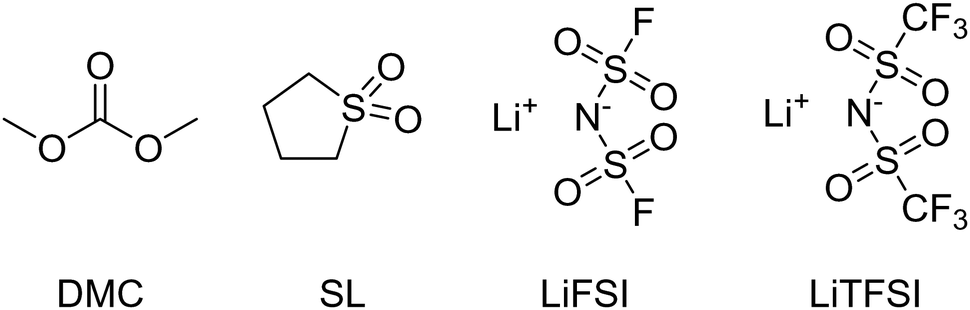 | ||
| Fig. 1 Molecular structures of used solvents (DMC and SL) and salts (LiFSI and LiTFSI). | ||
| Solvent | Salt | n solvent/nsalt | x solvent | x salt | c salt/mol l−1 |
|---|---|---|---|---|---|
| SL | LiTFSI | 2.0/1 | 0.67 | 0.33 | 2.94 |
| 3.0/1 | 0.75 | 0.25 | 2.31 | ||
| DMC | LiFSI | 1.1/1 | 0.52 | 0.48 | 5.48 |
| 1.3/1 | 0.57 | 0.43 | 5.04 | ||
| 2.0/1 | 0.67 | 0.33 | 3.90 | ||
Total ionic conductivity
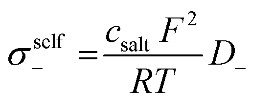
The total ionic conductivities of the electrolytes were determined using electrochemical impedance spectroscopy. A TSC 70 closed cell (RHD instruments, Darmstadt, Germany) was used in combination with an Alpha-A impedance analyzer (Novocontrol Technologies, Montabaur, Germany) equipped with a ZG2 interface. The measurements were carried out at 30 °C in a frequency range from 105 Hz to 1 Hz. A 0.1 M KCl standard solution was used to determine the cell constant k. The electrolyte resistance Rion was determined by fitting the obtained impedance spectra with the software RelaxIS (RHD instruments, Darmstadt, Germany). Ultimately, the total ionic conductivity σion was calculated according to σion = k/Rion.Very-low-frequency impedance spectroscopy on symmetric cells Li|electrolyte|Li
The transference numbers under anion blocking conditions and the salt diffusion coefficients were determined by very-low-frequency impedance spectroscopy (VLF). To this end, a symmetrical cell lithium|electrolyte|lithium with variable electrode distance was used as described in ref. 44. The cells were prepared in an argon-filled glovebox and electrochemical impedance measurements were carried out outside the glovebox with an Alpha-A impedance analyzer (Novocontrol Technologies) equipped with a ZG2 interface at a temperature of 30 °C. To ensure a stable interface between the electrodes and the electrolyte, an impedance spectrum in the frequency range 106 to 10−1 Hz was recorded every hour. If the change in interface resistance was less than 1 Ω h−1, the interface was considered stable and the VLF measurement was performed in a frequency range of 106 to 10−4 Hz with an applied AC voltage of 2 mVrms. This procedure was repeated at different electrode distances. By fitting the obtained VLF impedance spectra with the software RelaxIS (RHD instruments, Darmstadt, Germany) the Li+ transference number under anion-blocking conditions and the salt diffusion coefficient Dsalt were determined.
Concentration cell with transference
A concentration cell with transference was used to measure concentration-dependent open circuit potentials at 30 °C. The different components of the cell were stacked together in this order: Li|sample electrolyte with salt concentration csalt,|separator|reference electrolyte with salt concentration cref,|Li. The measurements were carried out as described before.41 By plotting the obtained open circuit potentials Δφ of different sample electrolytes against ln(csalt/c0) and performing a linear fit, the slope was acquired.
Density meausrements
Density measurements of the electrolytes were performed at 299.65 K using a DDM 2910 Automatic Density Meter (Rudolph Research Analytical, New York, USA). Prior to the measurements, removal of traces of water and oxygen was ensured by purging the instrument with dry nitrogen.Diffusion NMR and electrophoretic NMR
Multinuclear NMR measurements (7Li, 19F, 1H for Li, anion and solvent) were performed on an Avance Neo 400 MHz (Bruker, Rheinstetten, Germany) with a gradient probe head (Diff BB with maximum gradient strength of 17 T m−1 or 28 T m−1, rsp., Bruker). Inserting an NMR tube containing glycol and a PT100 thermocouple (GMH 3750, Greisinger, Regenstauf, Germany) into the spectrometer served to calibrate the temperature, which was set to 30 °C. Diffusion coefficients were obtained from a pulsed field gradient stimulated echo (PFGSTE) pulse sequence, taking a series of spectra with stepwise incremented gradient strength g. In each experiment the gradient pulse duration δ (1–3 ms) and observation time Δ (50–300 ms) were kept constant. This allows to evaluate the self-diffusion coefficient D according to eqn (1), where I is the signal intensity and γ is the gyromagnetic ratio of the respective nucleus. | (1) |
For the same nuclei and species, electrophoretic NMR (eNMR) experiments were carried out by applying an electric field to the sample, which was realized by immersing an electrode holder of custom design45 with an electrode distance of d = 2.2 cm into the liquid sample. A 1000 mc pulse generator (P&L Scientific, Sweden) was used to generate voltage pulses, which were implemented in a double stimulated echo (DSTE) pulse sequence46 and gradually increased with alternating sign, reaching a maximum that was adjusted individually for each sample, not exceeding 150 V for sulfolane-based samples and 100 V for DMC-based samples. In this series of spectra, the gradient pulse duration, gradient strength and observation time were kept constant at values optimized for each sample, which are in the range of δ = 1–3 ms, g up to 3.5 T m−1, and Δ = 50–100 ms. Migration of a species in the electric field leads to a phase shift Φ − Φ0 in the NMR spectrum, which was evaluated by phase-sensitive Lorentzian fits as described earlier.47 Then the mobility μ was determined from a linear fit of Φ − Φ0 against the voltage U according to eqn (2).
 | (2) |
For each sample a minimum of three repeated fillings of the eNMR electrode holder with fresh electrolyte were investigated, and the mobilities were averaged. The error was estimated as 5% plus additional statistical and fitting errors.
The mobility-based Li+ transference numbers were calculated from the ionic mobilities according to
 | (3) |
Overdetermination method for Onsager coefficients and thermodynamic factor
For the determination of four target quantities, namely three Onsager coefficients σ++, σ−− and σ+− and the thermodynamic factor , we used five experimental quantities σion,
  ,
,  , Dsalt and
  and applied the Monte Carlo-based overdetermination method described in ref. 41. This method leads to more accurate target values than the usual measurement of just four experimental quantities.41
Results and discussion
Experimental results and overdetermination method
In Fig. 2, diffusion coefficients for all species in the DMC/LiFSI system and in the SL/LiTFSI-system, respectively, are plotted versus the molar ratio nsolvent/nsalt. The latter are in the same range as in an earlier publication.32 In all systems, the diffusion coefficients decrease with increasing lithium salt concentration due to increasing Coulombic interactions. In the DMC-based systems, the DMC solvent is the fastest diffusing species, while the anion and Li+ ion diffusion is similar. In the SL/LiTFSI-system, Li+ ions and solvent molecules diffuse faster than the anions. Diffusion coefficients for the SL/LiFSI-system were published earlier and also show Li+ as the fastest diffusing species.41 | ||
| Fig. 2 Diffusion coefficients of solvent molecules (green squares), lithium ions (purple dots) and anions (orange triangles) in the DMC/LiFSI electrolytes and in the SL/LiTFSI electrolytes, respectively. | ||
In Fig. 3, we plot the ionic conductivities of all electrolytes versus the molar ratio nsolvent/nsalt. In all three systems, the ionic conductivity decreases with increasing salt concentration. At the same molar ratio nsolvent/nsalt = 2, the DMC/LiFSI electrolyte exhibits a considerably higher ionic conductivity (3.6 mS cm−1) than the SL/LiTFSI electrolyte (0.42 mS cm−1). This difference is related to the higher melting temperature of SL-based electrolytes as compared to DMC-based electrolytes. Pure SL exhibits a melting temperature of 27.5 °C and a viscosity of n = 10.34 mPa s at 30 °C,27 while DMC exhibits a melting temperature of 4 °C and a viscosity of 0.59 mPa s at 30 °C.25 This suggests stronger intermolecular interactions and slower dynamics in SL-based systems as compared to DMC-based systems.
 | ||
| Fig. 3 Ionic conductivities of the electrolytes plotted versus the molar ratio nsolvent/nsalt. | ||
In Fig. 4, we show electrophoretic mobilities of all species in the DMC/LiFSI and the SL/LiTFSI systems, respectively. Representative eNMR phase shift data used for calculating the electro-phoretic mobilities are shown in the ESI,† see Fig. S1 and S2. Electrophoretic mobility data for the SL/LiFSI system were already published in ref. 41. Similar mobility values in the DMC/LiFSI system were obtained by Bergstrom and McCloskey.40 As shown in Fig. S3 of the ESI,† ionic conductivities calculated from the ion mobilities are in good agreement with ionic conductivities obtained from impedance spectroscopy. As seen from Fig. 4, Li+ ions and anions show a drift direction expected from their individual sign of charge, while the solvent molecules show a positive drift direction, i.e. they move in the same direction as the Li+ ions.
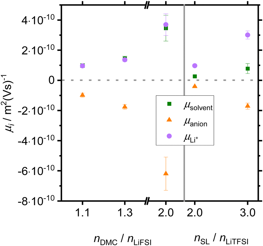 | ||
| Fig. 4 Electrophoretic mobilities of solvent molecules (green squares), Li+ ions (purple dots) and anions (orange triangles) plotted versus the molar ratio nsolvent/nsalt. | ||
Values for the mobility-based Li+ transference number  of the DMC/LiFSI-and SL/LiTFSI-electrolytes are shown in Fig. 5. In the DMC/LiFSI system,
  increases from 0.37 at x = 2 to 0.49 at x = 1.1, while in the SL/LiTFSI system,
  is in the range from 0.64–0.70. Similar results with
  were found for the SL/LiFSI system.41
 | ||
| Fig. 5 Mobility-based Li+ transference numbers of DMC/LiFSI electrolytes and SL/LiTFSI electrolytes calculated from the electrophoretic mobilities shown in Fig. 4 are plotted versus the molar ratio nsolvent/nsalt. | ||
Results obtained for the transference number under anion blocking conditions  , the salt diffusion coefficient Dsalt and the OCP slope
  are given in Table 2 together with the ionic conductivities and the mobility-based Li+ transference numbers. The table also contains data for SL/LiFSI published earlier,41 allowing direct comparison of the effect of the anion (SL/LiTFSI vs. SL/LiFSI) and the effect of the solvent (SL/LiFSI vs. DMC/LiFSI).
| System | n solvent/nsalt |
|
σ ion/mS cm−1 | t abc+ | D salt/10−11 m2 s−1 |
|
|---|---|---|---|---|---|---|
| SL/LiTFSI | 2.0/1 | (0.70 ± 0.09) | (0.42 ± 0.03) | (0.50 ± 0.08) | (3.0 ± 1.0) | (0.15 ± 0.04) |
| 3.0/1 | (0.64 ± 0.07) | (0.98 ± 0.06) | (0.32 ± 0.03) | (3.3 ± 0.5) | (0.09 ± 0.02) | |
| SL/LiFSI41 | 2.4/1 | (0.66 ± 0.10) | (1.56 ± 0.13) | (0.23 ± 0.02) | (1.2 ± 0.2) | (0.091 ± 0.015) |
| 3.0/1 | (0.56 ± 0.11) | (1.94 ± 0.04) | (0.29 ± 0.02) | (3.2 ± 0.9) | (0.073 ± 0.017) | |
| DMC/LiFSI | 1.1/1 | (0.49 ± 0.06) | (0.98 ± 0.03) | (0.37 ± 0.08) | (0.6 ± 0.2) | (0.14 ± 0.04) |
| 1.3/1 | (0.44 ± 0.04) | (1.51 ± 0.06) | (0.32 ± 0.08) | (2.1 ± 0.8) | (0.15 ± 0.07) | |
| 2.0/1 | (0.37 ± 0.09) | (3.63 ± 0.15) | (0.28 ± 0.02) | (5.3 ± 0.9) | (0.17 ± 0.03) | |


Using these five experimental quantities, the Monte Carlo-based overdetermination method described in ref. 41 yields a distribution for each of the three Onsager coefficients σ++, σσ−−, and σ+− as well as the thermodynamic factor (TF), from which the mean value and an uncertainty for each parameter can be determined. Fig. S9 in the ESI,† shows a representative distribution for the DMC/LiFSI 1.1![[thin space (1/6-em)]](https://www.rsc.org/images/entities/char_2009.gif) :1 and SL/LiTFSI 3.0/1 system. In Table 3, the Onsager coefficients normalized to the respective ionic conductivity are listed together with the uncertainties obtained from the Monte Carlo-based method.
:1 and SL/LiTFSI 3.0/1 system. In Table 3, the Onsager coefficients normalized to the respective ionic conductivity are listed together with the uncertainties obtained from the Monte Carlo-based method.
| System | n solvent/nsalt | σ ++/σion | σ −−/σion | σ +−/σion | TF |
|---|---|---|---|---|---|
| SL/LiTFSI | 2.0/1 | (0.55 ± 0.08) | (0.32 ± 0.17) | (−0.12 ± 0.09) | (5.6 ± 1.2) |
| 3.0/1 | (0.41 ± 0.04) | (0.32 ± 0.10) | (−0.15 ± 0.04) | (4.8 ± 0.7) | |
| SL/LiFSI41 | 2.4/1 | (0.36 ± 0.06) | (0.26 ± 0.08) | (−0.19 ± 0.02) | (4.3 ± 0.7) |
| 3.0/1 | (0.39 ± 0.02) | (0.28 ± 0.02) | (−0.16 ± 0.02) | (3.7 ± 0.8) | |
| DMC/LiFSI | 1.1/1 | (0.38 ± 0.06) | (0.37 ± 0.09) | (−0.13 ± 0.04) | (4.7 ± 0.9) |
| 1.3/1 | (0.37 ± 0.06) | (0.51 ± 0.09) | (−0.06 ± 0.06) | (5.2 ± 1.0) | |
| 2.0/1 | (0.30 ± 0.03) | (0.62 ± 0.11) | (−0.04 ± 0.05) | (5.4 ± 0.8) | |
All electrolytes exhibit negative values of σ+−, i.e. cations and anions move in an anticorrelated fashion. The relevance of these anticorrelations can be quantified by calculating the parameter β19,44 as
 | (4) |
Based on the β values, see Table 4, it can be concluded that the SL-based electrolytes exhibit stronger cation–anion anticorrelations than the DMC-based electrolytes. Furthermore, the role of the anticorrelations increases in almost all cases with rising salt concentration.
| System | n solvent/nsalt | σ self+/mS cm−1 | σ self−/mS cm−1 | σ distinct++/σ+self | σ distinct−−/σ−self | β |
|---|---|---|---|---|---|---|
| SL/LiTFSI | 2.0/1 | (0.37 ± 0.03) | (0.24 ± 0.03) | (−0.38 ± 0.15) | (−0.44 ± 0.38) | (−0.28 ± 0.22) |
| 3.0/1 | (0.9 ± 0.1) | (0.64 ± 0.08) | (−0.53 ± 0.16) | (−0.51 ± 0.22) | (−0.41 ± 0.12) | |
| SL/LiFSI41 | 2.4/1 | (1.4 ± 0.1) | (0.98 ± 0.05) | (−0.60 ± 0.15) | (−0.59 ± 0.17) | (−0.61 ± 0.11) |
| 3.0/1 | (1.5 ± 0.2) | (1.3 ± 0.1) | (−0.51 ± 0.11) | (−0.57 ± 0.12) | (−0.48 ± 0.06) | |
| DMC/LiFSI | 1.1/1 | (1.20 ± 0.08) | (1.17 ± 0.08) | (−0.69 ± 0.10) | (−0.69 ± 0.12) | (−0.35 ± 0.12) |
| 1.3/1 | (1.9 ± 0.1) | (1.9 ± 0.2) | (−0.70 ± 0.11) | (−0.59 ± 0.13) | (−0.14 ± 0.14) | |
| 2.0/1 | (4.5 ± 0.2) | (5.1 ± 0.3) | (−0.76 ± 0.09) | (−0.56 ± 0.12) | (−0.09 ± 0.11) | |
Next, we split the Onsager coefficients σ++ and σ−− into their self parts and distinct parts by making use of the measured self diffusion coefficients (listed in Table S1 of the ESI†):19
 | (5) |
 | (6) |
| σdistinct++ = σ++ − σself+ | (7) |
| σdistinct−− = σ−− − σself− | (8) |
In Table 4, we list the distinct parts of the Onsager coefficients, all normalized to their respective self part. This normalized quantity describes by what fraction an Onsager coefficient is reduced relative to its self part by like-ion anticorrelations. As seen from Table 4, all electrolytes exhibit strong cation–cation and anion–anion anticorrelations. These findings are in stark contrast to Onsager coefficients determined for the SL/LiTFSI system by MD simulations.35 The mismatch highlights once more the benefit of the precise quantification of the Onsager coefficients by the overdetermination method.
Volume conservation and dynamic correlations of the solvent
The above presented Onsager coefficients are derived for the ionic constituents, but a further analysis of the role of the solvent by its molecular correlations or anticorrelations can shed further light on the ion transport mechanisms. The analysis we propose here is based on mobility data of the respective solvent, and on the fact that volume conservation governs the fluxes of all species, as recently shown for concentrated electrolytes.42 The net volume flux JV was calculated by using the partial molar volumes νi of all species i (see ESI,† Table S4) and their measured mobilities μi. The calculation of the partial molar volumes of all species νi is described in detail in the ESI.† The net volume flux JV was normalized by the sum of the absolute values of the individual volume fluxes, JV,tot, in order to obtain a measure for the magnitude of the net volume flux.42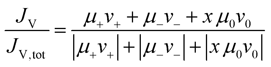 | (9) |
As shown in Fig. S10 of the ESI,† the normalized volume flux JV/JV,tot is close to zero for the DMC/LiFSI and SL/LiTFSI electrolytes. The same was demonstrated already for the SL/LiFSI system.41 This indicates that volume conservation plays an essential role for the dynamics of ions and molecules in highly concentrated electrolytes.
Since we approximate the partial molar volume of the Li+ ions, νLi+, by their molar volume VM,Li+, and since νLi+ is about two orders of magnitude smaller than the experimentally determined partial molar volumes of the salts, νsalt, and of the solvents, ν0, the partial molar volume of the Li+ ions can be neglected for the calculation of the solvent-related Onsager coefficients. Together with the restriction of volume conservation this leads to the following relations between Onsager coefficients, as shown in the ESI† (eqn (S4)–(S8)):
 | (10) |
 | (11) |
 | (12) |
In the following, we discuss the physical meaning of eqn (10)–(12). When we consider an electrolyte in thermal equilibrium, a movement of an anion or of a solvent molecule involves a shift of its volume. In order to prevent a local compression in the basically incompressible electrolyte, a correlated movement of other anions or other solvent molecules to compensate the volume drift is required. On the one hand, this implies anticorrelated movements of anions and molecules as sketched in Fig. 6(i). Accordingly, the Onsager coefficient σ−0 is always negative as described by eqn (10). On the other hand, volume conservation can also be achieved by anion–anion anticorrelations and by solvent–solvent anticorrelations as sketched in Fig. 6(ii) and (iii), respectively. Solvent–solvent anticorrelations can be analyzed by splitting the Onsager coefficient σ00 = σself0 + σdistinct00 into its self part  and its distinct part σdistinct00. Solvent–solvent anticorrelations and anion–anion anticorrelations lead to negative values of σdistinct00 and σdistinct−−, respectively. In the electrolytes considered here, we have σself0 > σself− due to the higher solvent concentration. Consequently, in the case of an electrolyte with a similar volume of the anion and the solvent molecule and accordingly σ00 ≈ σ−− (eqn (11)), the distinct part σdistinct00 has to be negative with a larger magnitude than σdistinct−−. Thus, in diluted electrolytes with a high molar solvent fraction x, solvent–solvent anticorrelations are mainly responsible for volume conservation, while with increasing salt concentration, anion–anion anticorrelations play an increasingly important role for volume conservation.
 | ||
| Fig. 6 Schematic illustration of anticorrelated movements leading to volume conservation in an electrolyte: (i) a solvent molecule is exchanged by an anion (ii) a solvent molecule is exchanged by another solvent molecule (iii) an anion is exchanged by another anion. | ||
Since the volume of the Li+ ions is negligible, Li+ ion movements only play a role for volume conservation, if these movements are correlated with the movements of anions or solvent molecules. Such correlations can be caused by Li+–solvent and Li+–anion interactions. If the Li+–solvent interactions are stronger than the Li+–anion interactions, Li+ ions move preferentially into the same direction as the solvent molecules, leading to σ+0 > 0. For volume conservation reasons, anions have to move into the opposite direction, resulting in σ+− < 0, as described by eqn (12). In contrast, if the Li+–anion interactions are stronger, Li+ ions and anions move preferentially into the same direction, while solvent molecules moving preferentially into the opposite direction, leading to σ+− > 0 and σ+0 < 0.
We note that the Onsager coefficient σ+0 gives direct information on the relevance of a vehicular Li+ transport mechanism, which is frequently discussed in the literature.37,48,49 In the case of a strictly vehicular Li+–solvent transport, all solvent molecules move together with the Li+ ion they are bound to, so that the displacement vector of a Li+ ion and the displacement vectors of the x solvent molecules bound to this Li+ ions are identical. In the ESI,† we show that in this case, the equation  is valid, see derivation in eqn (S9)—(S16) in the ESI.† Consequently, we define a parameter γ as
 | (13) |
 | ||
| Fig. 7 (a) If the Li+–solvent interactions are stronger than the Li+–anion interactions, Li+ move preferentially into the same direction as the solvent molecules, leading to a vehicular transport mechanism. (b) If the Li+–solvent interactions and the Li+–anion interactions are balanced, Li+ movements and solvent movements are uncorrelated. | ||
Influence of anion type on correlations
In the following, we analyze the influence of the anion in the two sulfolane-based electrolytes on the ion correlations. We compare two electrolytes with the same solvent-to-salt ratio (SL/LiTFSI or SL/LiFSI 3.0/1) as well as two electrolytes with salt concentrations at the solubility limit (SL/LiTFSI 2.0/1 and SL/LiFSI 2.4/1). For all sulfolane-based electrolytes, we find σ++ > σ−−, i.e., consistent with the magnitude of the mobilities (Fig. 4), the cations are more mobile than the anions. Furthermore, all sulfolane-based electrolytes exhibit negative values of σ+−, revealing anticorrelated movements of Li+ ions and anions. At the same solvent to salt ratio of 3.0/1, a slightly lower magnitude of the β value (−0.41, Table 4) is obtained for the SL/LiTFSI system as compared to the SL/LiFSI system (−0.48). However, this difference is small compared to the uncertainty of the β values. At higher salt concentrations at the solubility limit, however, the influence of the anion type on β is much stronger, namely β = −0.61 for SL/LiFSI 2.4/1 compared to β = −0.28 for SL/LiTFSI 2.0/1. This can be rationalized by considering the lack of solvent molecules for the solvation of the Li+ ions at high salt concentrations. This lack implies a higher relevance of the Li+–anion interaction strength for the structure and dynamics of the electrolyte. The stronger Li+–TFSI− attractive interaction as compared to the Li+–FSI− interaction50–54 should reduce the cation–anion anticorrelations in SL/LiTFSI 2.0/1 more as compared to SL/LiFSI 2.4/1. Thus, the attractive Li+–anion interaction counteracts the volume conservation which is responsible for the cation–anion anticorrelations.Influence of solvent type on correlations
In order to elucidate the influence of the solvent on the correlations, we compare the SL/LiFSI system with the DMC/LiFSI system. The Onsager coefficients σ+0, σ−0 and σ00 were calculated by means of eqn (10)–(12) (ESI†) and are listed in Tables S5–S7 of the ESI.† In addition, the distinct part σdistinct00 was calculated and listed also in Tables S5–S7 (ESI†). As seen from these tables, the three quantities σ−0, σdistinct00 and σdistinct−− exhibit negative values for all systems. This is well in line with the expectations from volume conservation as discussed above (Fig. 6).The Onsager coefficient σ+0 is positive for all electrolytes. In order to classify the Li+ transport mechanism, we calculate the parameter γ according to eqn (13) (ESI†). In Fig. 8, the parameter γ is plotted versus the molar ratio nsolvent/nsalt. The γ values are below 0.4 for all electrolytes, implying that Li+ transport is closer to the uncorrelated mechanism than to a vehicular mechanism. For a given molar ratio, the SL-based electrolytes exhibit higher γ values than the DMC-based electrolytes. The electrolyte SL/LiFSI system with a molar ratio of 2.4/1 exhibits the highest value with γ = 0.38. This gives strong indication that in the SL-based electrolytes, the Li+–SL interaction is stronger than the Li+–anion interaction. This can be rationalized by taking into account the high permittivity of SL as the solvent, which weakens the Li+–anion interactions. The significant amount of positive correlations between Li+ ion movements and solvent molecule movements in the sulfolane-based electrolytes observed in this experimental work challenges the Li+ hopping models proposed in the literature.31–33 According to eqn (S18) (ESI†), γ > 0 implies cation–anion anti-correlations with β < 0. These anticorrelations enhance charge transport, but slow down neutral salt transport.20,21
 | ||
| Fig. 8 Plot of the cation–solvent correlations parameter γ versus the molar ratio nsolvent/nsalt. The background colors indicate different transport mechanisms, i.e. green for predominantly vehicular Li+–solvent transport vs. brown for predominantly uncorrelated transport. | ||
The lowest value for γ is obtained for the DMC/LiFSI 2.0/1 electrolyte (γ = 0.09), which is the most dilute DMC-based electrolyte. The low value of γ implies that the Li+–DMC interactions and the Li+–anion interactions are virtually balanced. This can be rationalized by considering the lower permittivity of the DMC solvent as compared to SL. Since γ is close to zero, the cation–anion correlation parameter β is close to zero as well. In comparison to the negative value of β in SL-based electrolytes, this is advantageous for neutral salt transport, but is disadvantageous for charge transport.
As an example for an electrolyte with a pronounced vehicular mechanism we also calculated the parameter γ for an HCE consisting of a tetraglyme (G4) and LiFSI in a molar ratio of 1:1 (solvate ionic liquid, SIL), which we had already investigated in ref. 19. Since FSI− is a weakly coordinating anion, LiFSI-G4 should be close to a perfect SIL. The data are shown in Table S8 in the ESI.† The high γ value of 0.82 reflects the stable coordination of Li+ ions by single G4 molecules and the resulting strong vehicular character of the Li+ transport. At molar ratios of G4 to salt of 1.5/1 and 2/1 i.e. at lower salt concentrations the value for γ is lowered to 0.54 and 0.42, respectively. This indicates that the vehicular character of the Li+ transport decreases with increasing G4-to-salt molar ratio, which is in good agreement with the existing literature on glyme-based electrolytes, and it highlights the virtue of the new parameter γ for quantifying the degree of vehicular transport. It should be noted, however, that not all Li salt/G4 mixtures give perfect SILs.
The weaker cation–anion anticorrelations in the DMC-based electrolytes as compared to the SL-based electrolytes manifest also in the Haven ratio of these electrolytes, which is defined as:
 | (14) |
 | (15) |
Using this equation, the influence of like-ion anticorrelations and of cation–anion correlations, respectively, on the Haven ratio can be analyzed separately, as illustrated in Fig. 9. The cation–cation anticorrelations (C–C) and the anion–anion anticorrelations (A–A) lead to a strong drop of HR−1, i.e. to a strong increase of HR. This implies that like-ion anticorrelations lower the ionic conductivity for given diffusion coefficients of the ions. For both electrolytes, the influence of these like-ion anticorrelations is similar. In contrast, cation–anion anticorrelations enhance HR−1 and thus the ionic conductivity for given diffusion coefficients of the ions. As seen from Fig. 9, the stronger cation–anion anticorrelations in the electrolyte SL/LiFSI 2.4/1 are advantageous for the ionic conductivity as manifested in a higher value of HR−1.
 | ||
| Fig. 9 Schematic illustration of the influence of cation–cation (C–C) anticorrelations, anion–anion (A–A) anticorrelations, and cation–anion (C–A) anticorrelations on the inverse Haven ratio HR−1 of the two electrolytes SL/LiFSI 2.4/1 and DMC/LiFSI 2.0/1. | ||
Conclusions
We have applied an experimental overdetermination method for obtaining accurate values for the Onsager coefficients σ++, σ−−, σ+− and for the thermodynamic factor of highly concentrated binary electrolytes. The electrolytes were composed of either sulfolane or dimethyl carbonate as solvent and of either LiTFSI or LiFSI as salt. Electrophoretic NMR results together with partial molar volume data gave strong indication that the transport in all electrolytes is governed by volume conservation. Based on this governing constraint, the solvent-related Onsager coefficients σ+0, σ−0, and σ00 were calculated. All Onsager coefficients were analyzed with regard to the influence of the salt anion and of the solvent on dynamic correlations and transport mechanisms. To this end, a parameter γ was defined, which is a measure for the relevance of a vehicular Li+–solvent transport mechanism. In the case of sulfolane-based electrolytes, the Li+–sulfolane interactions are significantly stronger than the Li+–anion interactions. This leads to a γ parameter up to 0.38, suggesting a significant relevance of vehicular Li+–sulfolane transport. In this case, volume conservation implies cation–anion anticorrelations, which are advantageous for charge transport, but disadvantageous for neutral salt transport in a battery. In contrast, in the case of DMC-based electrolytes, Li+–DMC and Li+–anion interactions are similar in strength. This leads to virtually uncorrelated transport of Li+ ions and DMC molecules manifested in a γ parameter close to zero.
Data availability
Data supporting this article have been included as part of the ESI.†Conflicts of interest
There are no conflicts to declare.Acknowledgements
We would like to thank the German Science Foundation (DFG) for financial support of this work under the project numbers Ro1213/19-1 and Scho 636/8-1 (project no. 504905154). Maleen Middendorf is supported by the International Graduate School for Battery Chemistry, Characterization, Analysis, Recycling and Application (BACCARA), which is funded by the Ministry for Culture and Science of North Rhine Westphalia, Germany. The NMR experiments were performed on spectrometers funded by the Deutsche Forschungsgemeinschaft (DFG, German Research Foundation), project numbers 610758 and 452849940.Notes and references
- B. Flamme, G. Rodriguez Garcia, M. Weil, M. Haddad, P. Phansavath, V. Ratovelomanana-Vidal and A. Chagnes, Green Chem., 2017, 19(8), 1828 RSC
.
- K. Xu, Chem. Rev., 2004, 104(10), 4303 CrossRef CAS PubMed
- O. Borodin, J. Self, K. A. Persson, C. Wang and K. Xu, Joule, 2020, 4(1), 69 CrossRef CAS
- S. Hess, M. Wohlfahrt-Mehrens and M. Wachtler, J. Electrochem. Soc., 2015, 162(2), A3084–A3097 CrossRef CAS
- E. P. Roth and C. J. Orendorff, Interface, 2012, 21(2), 45 CAS
- A. Mauger and C. M. Julien, Ionics, 2017, 23(8), 1933 CrossRef CAS
- Y. Chen, Y. Kang, Y. Zhao, L. Wang, J. Liu, Y. Li, Z. Liang, X. He, X. Li, N. Tavajohi and B. Li, J. Energy Chem., 2021, 59, 83 CrossRef
- N. Nitta, F. Wu, J. T. Lee and G. Yushin, Mater. Today, 2015, 18(5), 252 CrossRef
- A. Manthiram, ACS Cent. Sci., 2017, 3(10), 1063 CrossRef PubMed
- N. P. W. Pieczonka, Z. Liu, P. Lu, K. L. Olson, J. Moote, B. R. Powell and J.-H. Kim, J. Phys. Chem. C, 2013, 117(31), 15947 CrossRef
- J. Wang, Y. Yamada, K. Sodeyama, C. H. Chiang, Y. Tateyama and A. Yamada, Nat. Commun., 2016, 7, 12032 CrossRef
- Y. Yamada and A. Yamada, J. Electrochem. Soc., 2015, 162(14), A2406–A2423 CrossRef
- S.-A. Hyodo and K. Okabayashi, Electrochim. Acta, 1989, 34, 1551 CrossRef
- C. Zhang, K. Ueno, A. Yamazaki, K. Yoshida, H. Moon, T. Mandai, Y. Umebayashi, K. Dokko and M. Watanabe, J. Phys. Chem. B, 2014, 118(19), 5144 CrossRef PubMed
- J. S. Ho, O. A. Borodin, M. S. Ding, L. Ma, M. A. Schroeder, G. R. Pastel and K. Xu, Energy Environ. Mater., 2023, 6(1), e12302 CrossRef
- J. Neuhaus, E. von Harbou and H. Hasse, J. Power Sources, 2018, 394, 148 CrossRef
- K. D. Fong, H. K. Bergstrom, B. D. McCloskey and K. K. Mandadapu, AIChE J., 2020, 66(12), e17091 CrossRef
- N. M. Vargas-Barbosa and B. Roling, ChemElectroChem, 2020, 7(2), 367 CrossRef
- S. Pfeifer, F. Ackermann, F. Sälzer, M. Schönhoff and B. Roling, Phys. Chem. Chem. Phys., 2021, 23(1), 628 RSC
- B. Roling, J. Kettner and V. Miß, Energy Environ. Mater., 2022, 5(1), 6 CrossRef
- B. Roling, V. Miß and J. Kettner, Energy Environ. Mater., 2024, 7(1), e12533 CrossRef
- L. Peter and J. Arai, J. Appl. Electrochem., 1999, 29, 1053 CrossRef
- Y. Yamada, C. H. Chiang, K. Sodeyama, J. Wang, Y. Tateyama and A. Yamada, ChemElectroChem, 2015, 2(11), 1687 CrossRef
- S.-K. Jeong, M. Inaba, Y. Iriyama, T. Abe and Z. Ogumi, J. Power Sources, 2008, 175(1), 540 CrossRef
- D. J. Schroeder, A. A. Hubaud and J. T. Vaughey, Mater. Res. Bull., 2014, 49, 614 CrossRef
- U. Tilstam, Org. Process Res. Dev., 2012, 16(7), 1273 CrossRef
- S. Li, B. Li, X. Xu, X. Shi, Y. Zhao, L. Mao and X. Cui, J. Power Sources, 2012, 209, 295 CrossRef
- A. Hofmann, M. Schulz, S. Indris, R. Heinzmann and T. Hanemann, Electrochim. Acta, 2014, 147, 704 CrossRef
- S.-Y. Lee, K. Ueno and C. A. Angell, J. Phys. Chem. C, 2012, 116(45), 23915 CrossRef
- J. Alvarado, M. A. Schroeder, M. Zhang, O. Borodin, E. Gobrogge, M. Olguin, M. S. Ding, M. Gobet, S. Greenbaum, Y. S. Meng and K. Xu, Mater. Today, 2018, 21(4), 341 CrossRef
- K. Dokko, D. Watanabe, Y. Ugata, M. L. Thomas, S. Tsuzuki, W. Shinoda, K. Hashimoto, K. Ueno, Y. Umebayashi and M. Watanabe, J. Phys. Chem. B, 2018, 122(47), 10736 CrossRef PubMed
- A. Nakanishi, K. Ueno, D. Watanabe, Y. Ugata, Y. Matsumae, J. Liu, M. L. Thomas, K. Dokko and M. Watanabe, J. Phys. Chem. C, 2019, 123(23), 14229 CrossRef
- Y. Ugata, S. Sasagawa, R. Tatara, K. Ueno, M. Watanabe and K. Dokko, J. Phys. Chem. B, 2021, 125(24), 6600 CrossRef PubMed
- K. Shigenobu, K. Dokko, M. Watanabe and K. Ueno, Phys. Chem. Chem. Phys., 2020, 22(27), 15214 RSC
- S. Ikeda, S. Tsuzuki, T. Sudoh, K. Shigenobu, K. Ueno, K. Dokko, M. Watanabe and W. Shinoda, J. Phys. Chem. C, 2023, 127(28), 13837 CrossRef
- O. Borodin and G. D. Smith, J. Solution Chem., 2007, 36(6), 803 CrossRef
- A. Mistry, Z. Yu, L. Cheng and V. Srinivasan, J. Electrochem. Soc., 2023, 170(11), 110536 CrossRef
- R. Andersson, F. Årén, A. A. Franco and P. Johansson, J. Electrochem. Soc., 2020, 167(14), 140537 CrossRef
- D. Dong, F. Sälzer, B. Roling and D. Bedrov, Phys. Chem. Chem. Phys., 2018, 20(46), 29174 RSC
- H. K. Bergstrom and B. D. McCloskey, ACS Energy Lett., 2024, 9(2), 373 CrossRef PubMed
- T. Pothmann, M. Middendorf, C. Gerken, P. Nürnberg, M. Schönhoff and B. Roling, Faraday Discuss., 2024, 253, 100 RSC
- M. Lorenz, F. Kilchert, P. Nürnberg, M. Schammer, A. Latz, B. Horstmann and M. Schönhoff, J. Phys. Chem. Lett., 2022, 13(37), 8761 CrossRef PubMed
- F. Kilchert, M. Lorenz, M. Schammer, P. Nürnberg, M. Schönhoff, A. Latz and B. Horstmann, Phys. Chem. Chem. Phys., 2023, 25(38), 25965 RSC
- F. Wohde, M. Balabajew and B. Roling, J. Electrochem. Soc., 2016, 163(5), A714–A721 CrossRef
- M. Gouverneur, J. Kopp, L. van Wüllen and M. Schönhoff, Phys. Chem. Chem. Phys., 2015, 17(45), 30680 RSC
- A. Jerschow and N. Müller, J. Magn. Reson., 1997, 125(2), 372 Search PubMed
- F. Schmidt, A. Pugliese, C. C. Santini, F. Castiglione and M. Schönhoff, Magn. Reson. Chem., 2020, 58(3), 271 CrossRef CAS PubMed
- M. Brinkkötter, G. A. Giffin, A. Moretti, S. Jeong, S. Passerini and M. Schönhoff, Chem. Commun., 2018, 54(34), 4278 RSC
- M. Gouverneur, F. Schmidt and M. Schönhoff, Phys. Chem. Chem. Phys., 2018, 20(11), 7470 RSC
- J. B. Haskins, W. R. Bennett, J. J. Wu, D. M. Hernández, O. Borodin, J. D. Monk, C. W. Bauschlicher and J. W. Lawson, J. Phys. Chem. B, 2014, 118(38), 11295 CrossRef
- L. Wang, Z. Luo, H. Xu, N. Piao, Z. Chen, G. Tian and X. He, RSC Adv., 2019, 9(71), 41837 RSC
- X. Chen and D. G. Kuroda, Chem. Commun., 2023, 59(13), 1849 RSC
- M. Brinkkötter, A. Mariani, S. Jeong, S. Passerini and M. Schönhoff, Adv. Energy Sustainability Res., 2021, 2(2), 2000078 CrossRef
- M. Lorenz and M. Schönhoff, J. Phys. Chem. B, 2024, 128(11), 2782 CrossRef
Footnotes |
| † Electronic supplementary information (ESI) available. See DOI: https://doi.org/10.1039/d4cp04209c |
| ‡ H. K. and T. P. contributed equally to this work. |
| This journal is © the Owner Societies 2025 |