A chemometric approach for the design of lanthanum-based high entropy perovskite oxides

Abstract

Nowadays, the existence of high entropy perovskite (HEP) oxides is well established and, since their discovery, they have found application in several technological fields. The main advantage provided by these materials, with the general formula ABO₃, is the possibility of widely tuning their properties by acting on the chemical composition. The study of stability, fields of existence, and solubility limits in a systematic way remains lacking in comparison with continuous application research, despite the presence of large datasets and computational studies. In the present work, we aimed at investigating the structure and solubility limits of two series of HEPs including five different cations on the perovskite B-site, namely La(CrMnFeCoNi)O₃ and La(CrMnFeCoZn)O₃, exploring a full range of compositions beyond the classical equimolar phases usually investigated. This has been accomplished by the design of experiment strategy to investigate the influence of the B-site composition on phase stability, crystal structure, and oxygen non-stoichiometry for the two systems providing a solid tool for researchers to predict such properties on the whole compositional space of the two HEPs.

---

Introduction

From the discovery of high entropy materials, research has shifted to investigate an ever-increasing number of samples in order to identify the best performing ones for any given application. This class of materials has proved to be useful in the fields of alloys, oxides, and perovskites due to their high tunability by acting on the chemical compositions.^1–4 The fundamental principle underlying the high-entropy stabilization concept centers on the combination of a substantial number of cations, typically five or more, within a solid solution, distributed in equimolar proportions.^5,6 This unique approach often leads to the formation of a single-phase structure, effectively overcoming the enthalpy-driven phase separation challenges frequently encountered in heavily doped systems. Unlike traditional scenarios where compounds tend to exhibit phase separation, the high-entropy concept allows for the creation of single-phase compounds with compositions positioned at the center of intricate phase diagrams—regions that are seldom explored in conventional studies. The stabilization of these compounds is achieved through configurational entropy, and a distinctive feature is their increased stability with rising temperatures.^7,8 This innovative approach has facilitated the production of diverse compositions, each characterized by different elemental combinations and resulting in a variety of crystal structures. Among these structures we find rock salt, fluorite, spinels, and perovskites, illustrating the versatility and effectiveness of the high-entropy approach in stabilizing materials with distinct and often unexplored properties.⁹ Consequently, the high-entropy stabilization concept opens avenues for the investigation of novel single-phase compounds, providing valuable insights into their thermodynamic and structural behaviors, especially in regions of complex phase diagrams that have been historically underexplored.

Among the relatively vast examples of high entropy oxides (HEOs) explored to date, a clear understanding has emerged, i.e. the configurational entropy plays a dominant role in determining the Gibbs free energy of formation.^7,10,11 This entropy effectively compensates for any positive enthalpic contributions, showcasing the pivotal influence of configurational entropy in stabilizing these high-entropy materials.^12,13 The configurational entropy of a system experiences a notable increase as the number of different elements distributed over the cation lattice site rises, reaching its maximum when all constituent elements are present in equimolar amounts.¹⁴ Beyond the intriguing structural implications, this distinct design concept not only highlights the significance of configurational entropy but also presents an opportunity for fine-tuning of materials functional properties.^5,15,16 The equimolar distribution of diverse elements creates a unique environment wherein the interplay of configurational entropy and elemental composition contributes to the overall stability and properties of the high-entropy materials. This nuanced understanding not only expands our comprehension of the thermodynamic aspects but also opens avenues for tailoring functional characteristics in a controlled manner, providing a promising platform for the development of materials with finely tuned and optimized properties.^17–22 Most of these studies are based on a computational or machine learning approach where potential chemistries are interpolated and compared in order to predict the structure and performance of a huge number of materials. However, only equimolar quantities with a high number of cations are mostly considered in these approaches leaving the experimental part deficient, often without real feedback, and failing in emphasizing the influence and synergy between cations.^23–25

To address some of these issues, in the current investigation we focused on the rational characterisation of ABO₃ perovskites in which B sites are occupied by a combination of Cr, Mn Fe, Co and either Ni or Zn in order to unveil the effect of the type and quantity of cations (moving beyond equimolar compositions) occupying B sites on specific perovskite properties, such as the phase composition, structural geometry, and oxygen non-stoichiometry. This has been evaluated by means of the design of experiment tool. Concurrently, relying on a suitable training set of perovskites whose compositions have been selected by D-optimal design, polynomial models are developed and validated to allow the prediction and optimisation of the properties of interest within the entire experimental domain.

As mentioned above, the materials under scrutiny encompass compositions ranging from two- to six-element mixtures. Despite the proximity of these elements in the periodic table, their inclusion introduces variability in redox capacities and oxygen vacancies within the material structures. A key distinction between the two sets lies in the behavior of Ni and Zn: Ni has the capacity to be oxidized to Ni³⁺, whereas Zn can only exist in the Zn²⁺ oxidation state. This difference leads to the generation of vacancies, compelling other elements to adapt to the presence of Zn as a dopant within the structure. Additionally, a common dataset is considered, comprising samples that exclude both nickel and zinc. Leveraging chemometric analysis, we systematically mapped all conceivable combinations of these cations. This mapping encompasses a spectrum ranging from end-members, characterized by samples with only one cation on the A site and one on the B site, to more complex members featuring five cations on the B site. Through this comprehensive compositional space mapping, we gain insights into the influence of each cation on the structural aspects and oxygen vacancies. Furthermore, we unravel the intricate synergy that emerges when these elements coexist within the material matrix. This rigorous experimental and chemometric approach not only sheds light on the structural intricacies of the studied compositions but also contributes to a deeper understanding of how different cations collaborate and influence the properties of high-entropy materials in a controlled and deliberate manner.

Result and discussion

Design of experiment approach for multicomponent materials

Considering the complexity of the systems under consideration, i.e. perovskite B-site occupied by up to 5 cations whose molar fraction can vary between 0 and 1, a trial-and-error approach is definitely time-consuming, simplistic and would result only in a local knowledge focused on the tested samples but can provide neither general information about the system nor prediction capability.²⁶ All these issues can be overcome by applying suitable multivariate tools generally included in the “design of experiments” approach (DOE): trying to generalise and summarise in few words this approach, the outcome of whatever experiment (response) depends on the experimental conditions (variables) according to a mathematical function y = f(x) that can be approximated by a polynomial function (model equation) that represents a good description of the correlation between response and variables in a limited experimental domain and allows also to predict the response value for non-tested experimental conditions, relying on the same already established correlations.²⁷ In this specific case, perovskite stability, crystal system and oxygen non-stoichiometry are the responses investigated while the molar fractions of the cations occupying site B represent the variables.

Depending on the type of variables, the response trend and the model equation postulated, different mathematical tools enable us to appropriately investigate any system, from the simplest cases to the most complex ones, but for further information on these techniques the readers should refer to the dedicated literature.^26–30 DOE has to be considered as an adaptable stepwise approach that, starting with the problem identification, leads to response modelling and prediction.³¹ The workflow followed for the rational characterisation of multicomponent ABO₃ perovskites is summarised in Fig. 1 and will be discussed in detail in the following sections and in the Experimental section (ESI†).

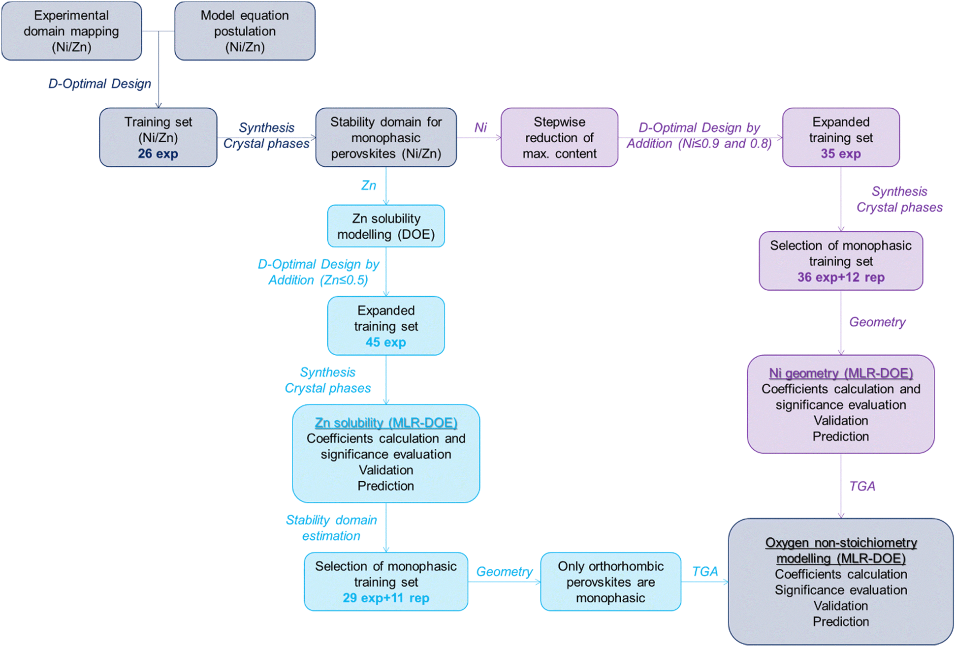Fig. 1 Workflow followed for rational characterisation of multicomponent ABO₃ perovskites.

Problem definition and training sample identification

Firstly, the experimental domain of interest is identified as the La(CrMnFeCoM)O₃ system, whereas M stands for Ni or Zn, in which each cation molar fraction is varied from 0 to 1. In order to treat the data through a chemometric approach, all perovskite systems were synthesized in the same way by a sol–gel synthesis starting from nitrate precursors followed by calcination at 750 °C for 6 hours, as described in detail in the ESI.† This experimental approach is commonly used in the current literature to prepare lanthanum-based perovskites and related high entropy phases.^32–34 This domain is homogeneously mapped by drawing up a list of all the possible combinations of the molar fractions of the five cations, using a minimum step of 0.1. This list is usually referred to as candidate point matrix (cp), reported in Table S1 (ESI†), and must represent a homogeneous mapping of the experimental domain since the samples to be synthesised and characterized are extracted from this list. Secondly, a suitable model equation has to be hypothesised, complex enough to represent the response trend in the domain but simple enough to reduce the number of experiments and avoid overfitting issues; according to background experience and previous knowledge on 5-component systems, we postulate the polynomial model reported in eqn (1), taking into account linear terms, 2-cations and 3-cations interactions.³⁵

y = b_Crx_Cr + b_Mnx_Mn + b_Fex_Fe + b_Cox_Co + b_Mx_M + b_CrMnx_Crx_Mn + b_CrFex_Crx_Fe + b_CrCox_Crx_Co + b_CrMx_Crx_M + b_MnFex_Mnx_Fe + b_MnCox_Mnx_Co + b_MnMx_Mnx_M + b_FeCox_Fex_Co + b_FeMx_Fex_M + b_CoMx_Cox_M + b_CrMnFex_Crx_Mnx_Fe + b_CrMnCox_Crx_Mnx_Co + b_CrMnMx_Crx_Mnx_M + b_CrFeCox_Crx_Fex_Co + b_CrFeMx_Crx_Fex_M + b_CrCoMx_Crx_Cox_M + b_MnFeCox_Mnx_Fex_Co + b_MnFeMx_Mnx_Fex_M + b_MnCoMx_Mnx_Cox_M + b_FenCoMx_Fex_Cox_M (1)

It glaringly appears that samples extracted from cp to train the model depend on the terms included in the polynomial model, both in term of numerosity, i.e. the more the number of terms included, the more the amount of samples required, and location in the domain, i.e. linear terms only require mono-cation samples while 2-cations and 3-cations interactions require the corresponding combinations. Once computed the candidate point matrix and the polynomial model, D-optimal design is employed to extract the best subset of training experiments from cp; being out of the purpose of this paper to describe in detail the algorithm besides this tool, only a qualitative description of the approach will be provided.³⁶ The algorithm iteratively identifies the best training set according to the D-optimality criterion, which means maximising the coefficients significance, their mutual independence and the information that can be extracted from the data. D-optimality is represented by a mathematical parameter that has to be normalized based on the number of experiments, since obviously a higher number of experiments always leads to higher information. The normalized parameter associated with the D-optimal set of training samples per each number of experiments is reported in Fig. S1 (ESI†) and the best compromises between extractable information and experimental effort are identified as the local maxima. In this case, 26-experimental solution, reported in Table S2 (ESI†), undoubtedly represents the preferable set of training experiments.

Stability domain estimation for single-phase La(Cr,Mn,Fe,Co,M)O₃ systems

Preliminary evaluation of perovskites stability. Training samples defined according to D-optimality criterion are synthesised according to the method reported in the experimental conditions and the percentage of perovskite phase is quantified by Rietveld refinement of the diffraction pattern for each sample. The results of the pattern refinements are listed in Table S2 (ESI†) for the 26-experiment training set while Fig. 2 reports two selected examples, namely LaMn_0.4(CrNi)_0.3O₃ and LaMn_0.4(CrZn)_0.3O₃. For all the samples discussed in the present manuscript, chemical composition has been determined by X-ray fluorescence spectroscopy (XRF) and found to be in very good agreement with the nominal composition.

Fig. 2 Rietveld refinement results for (a) LaMn_0.4(CrNi)_0.3O₃ and (b) LaMn_0.4(CrZn)_0.3O₃.

Just looking at the values obtained (Table S2, ESI†), we notice that Ni-containing perovskites are all single-phase, except for LaNiO₃, while Zn is much less soluble and results in several non-homogeneous materials, even for low Zn molar fractions. The difference between the two metals required a different approach, as summarised in Fig. 1.

For Ni-containing perovskites, according to the Rietveld refinement results on the 26 samples of the training set (Table S2, ESI†), the experimental domain is reduced to samples with Ni content below or equal firstly to 0.9, then to 0.8. In both cases, the cp in Table S1 (ESI†) is adapted to the new domains excluding samples out of these limits (Table S1, seventh and eight columns, ESI†) and the samples to be added to the first training set (Table S2, ESI†) are selected again according to D-optimality criterion. This latter tool is generally referred to as D-optimal design by addition and is often employed to amend or expand existing matrices whenever necessary.³⁵ The computed expanded training is reported in Table S3 (ESI†) and graphically represented in Fig. 3a in a pseudo-ternary domain in which the axes represent the molar fraction of Cr + Co, Mn + Fe and Ni. This Figure includes the results of the synthesis and structural characterization of the additional samples included in the expanded training set (results reported in Table S3, ESI†). At a glance, we can observe that single-phase samples (green) are obtained in almost the entire domain except for samples with Ni molar fraction equal to 1 and 0.9. Therefore, we can assume that single-phase perovskites are obtained for Ni content below or equal to 0.8.

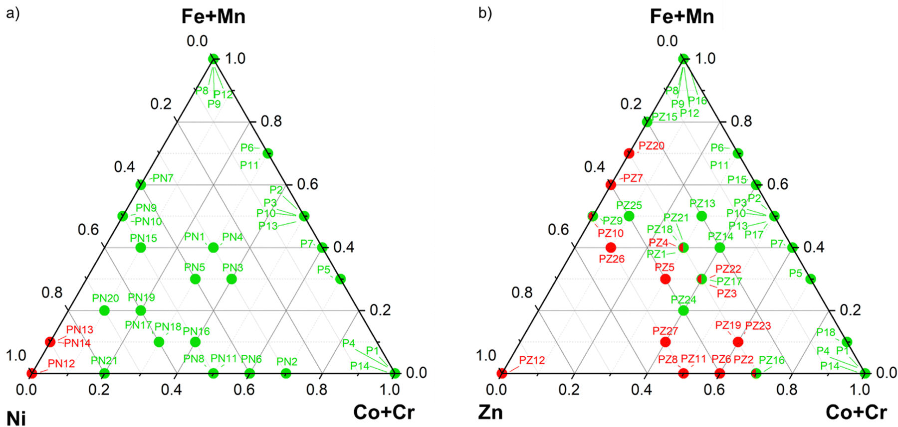Fig. 3 (a) Training samples (Table S3, ESI†) represented is a pseudo-ternary domain in which the axes are associated to the molar fraction of Cr + Co, Mn + Fe and Ni. Single-phase samples are labelled in green while the others in red; (b) training samples (Table S4, ESI†) represented is a pseudo-ternary domain in which the axis are associated to the molar fraction of Cr + Co, Mn + Fe and Zn. Single-phase samples are labelled in green while the others in red.

As can be appreciated by the results of the structural refinements reported in Table S2 (ESI†) for the La(Cr,Mn,Fe,Co,Zn)O₃ perovskites, the Zn solubility is much lower and strongly dependent on the other cations present and therefore we cannot perform a roughly estimation, as done in the case of Ni, but solubility should be modelled by Design of Experiments. Also in this case, D-optimal design by addition is applied to better investigate the region with Zn content below 0.5, since for higher Zn content single-phase materials are almost never achieved (see Table S2, ESI†). Analysing the percentage of perovskite for the expanded training set, reported in Table S4 (ESI†) and represented in Fig. 3b, we can confirm that single-phase materials are obtained only for low content of Zn but also the other cations do influence the stability of the phase.

Zn solubility in the perovskite system modelling. Having defined both the model equation and training samples list, properly selected by D-optimal design tools, the experimental values of perovskite percentage calculated for the 45 training samples (see Table S4, ESI†) are used to compute the coefficients in eqn (1) by means of multiple linear regression (MLR). The calculated coefficients, reported in Table S5 (ESI†) and represented in Fig. S2a (ESI†), properly approximate the response, explaining a sufficiently high percentage of experimental variance (E.V. = 94.10%), showing a low standard deviation for the fitting residuals (s = 4.68) and a good agreement between experimental and fitted values (Fig. S2b, ESI†). Computing coefficients significance relying on fitting residuals standard deviation, all the linear terms are found significant at 99.9% confidence level (***), as well as the interactions between Zn and Cr or Mn that both contribute in stabilising the perovskite phase. Some other Zn-containing interactions are found to exhibit a significant stabilisation effect such as Zn and Cr + Co, Mn + Co and Fe + Co (**, 99% C.L.) while the lowest significance is associated with Fe + Zn interaction (*, 95% C.L.). From the coefficients analysis, we can preliminarily hypothesize that Mn and Cr exhibit the highest stabilisation effect, followed by Fe and Co. Model validation is performed by comparing the experimental and predicted percentage of perovskite phase for thevalidation set reported in Table S6 (ESI†): the calculated Root Mean Square Error in Prediction (RMSEP = 0.61) is significantly lower than the fitting residuals standard deviation (s = 4.68) thus the model is validated (calculated F = 59.28, tabulated F_0.05,20,6 = 3.87). After validation, the b terms in eqn (1) can be replaced by computed coefficients in Table S5 (ESI†) obtaining the polynomial relating the experimental response, i.e. the percentage of perovskite, to the original variables, i.e. cations molar fraction. The so-obtained equation allows to predict the percentage of perovskite within the entire experimental domain, together with the associated confidence interval, but a comprehensive representation cannot be presented since 4 dimensions would be required to depict a 5-cations composition. Therefore, in Fig. 4 some partial representations of the predicted perovskite percentage are depicted, limiting the representation to ternary compositions including Zn and two other cations and plotting also the training samples referring to the given ternary composition. Both the predicted response and the experimental values are coloured according to the colourmap reported in Fig. 4 to ease the interpretation.

Fig. 4 Predicted perovskite percentage for La(Fe,Co,Zn)O₃ (left upper plot), La(Cr,Co,Zn)O₃ (right upper plot), La(Mn,Co,Zn)O₃ (left lower plot) and La(Cr,Mn,Zn)O₃ (right lower plot) and experimental values for the expanded training samples, all coloured according to the colourmap reported next to the ternary plots.

The ternary plot in Fig. 4 highlights the main points already hinted above: firstly, Zn solubility in the perovskite system strongly depends on the other cations included in the crystal and, secondly, Co and Fe exhibit the lower stabilisation effect while the presence of Cr and Mn allows to obtain single-phase materials for higher Zn amounts. In fact, phase pure La(Fe,Co,Zn)O₃ perovskites (ternary plot in the left upper part of Fig. 4) are predicted only for Zn molar fraction below 0.4, or even 0.2 for high Co contents, while the stability domain becomes wider replacing Fe with Cr (right upper plot), or even more with Mn (left lower plot). To conclude, La(Cr,Mn,Zn)O₃ perovskites is predicted to be single-phase for Zn content up to 0.5 thanks to the presence of the two most stabilising cations.

Selection of single-phase training samples and geometry modelling. As already discussed above, the lists of single-phase materials to be characterised is obtained by excluding multiphase samples from the expanded training sets reported in Tables S3 and S4 (ESI†): the ultimate lists of single-phase training samples is reported in Table 1 for La(Cr,Mn,Fe,Co,Ni)O₃ and in Table 2 for La(Cr,Mn,Fe,Co,Zn)O₃, together with the experimental values for the physicochemical properties of interest, namely the crystal structure (determined by refinement of the diffraction patterns) and the oxygen non-stoichiometry (determined by thermogravimetry – see the Experimental section, ESI†), δ (see later in the text).

Table 1 35-Experiments expanded training set for Ni-containing perovskites obtained by adding further experiments to the training set in Table S2 (ESI) extracted from the reduced cps (Table S1, seventh and eighth columns, ESI) by D-optimal design by addition

Sample	Formula	Cr	Mn	Fe	Co	Ni	Crystal System	δ
P1	LaCrO3	1	0	0	0	0	Orthorhombic	0.003
P2	La(CrMn)0.5O3	0.5	0.5	0	0	0	Orthorhombic	0.006
P3	La(CrFe)0.5O3	0.5	0	0.5	0	0	Orthorhombic	0.002
P4a	La(CrCo)0.5O3	0.5	0	0	0.5	0	Trigonal	0.027
P4b	La(CrCo)0.5O3	0.5	0	0	0.5	0	Trigonal	0.027
P5a	LaCr0.4(FeCo)0.3O3	0.4	0	0.3	0.3	0	Orthorhombic	0.005
P5b	LaCr0.4(FeCo)0.3O3	0.4	0	0.3	0.3	0	Orthorhombic	0.008
P5c	LaCr0.4(FeCo)0.3O3	0.4	0	0.3	0.3	0	Orthorhombic	0.002
P6	LaMn0.4(CrFe)0.3O3	0.3	0.4	0.3	0	0	Orthorhombic	0.011
P7	LaMn0.4(CrCo)0.3O3	0.3	0.4	0	0.3	0	Orthorhombic	0.002
P8	LaMnO3	0	1	0	0	0	Orthorhombic	0.006
P9a	La(MnFe)0.5O3	0	0.5	0.5	0	0	Orthorhombic	0.021
P9b	La(MnFe)0.5O3	0	0.5	0.5	0	0	Orthorhombic	0.018
P9c	La(MnFe)0.5O3	0	0.5	0.5	0	0	Orthorhombic	0.020
P10	La(MnFe)0.5O3	0	0.5	0	0.5	0	Orthorhombic	0.003
P11	LaMn0.4(FeCo)0.3O3	0	0.4	0.3	0.3	0	Orthorhombic	0.003
P12	LaFeO3	0	0	1	0	0	Orthorhombic	0.003
P13	La(FeCo)0.5O3	0	0	0.5	0.5	0	Trigonal	0.021
P14	LaCoO3	0	0	0	1	0	Trigonal	0.003
P15a	LaMn0.6Co0.4O3	0	0.6	0	0.4	0	Orthorhombic	0.024
P15b	LaMn0.6Co0.4O3	0	0.6	0	0.4	0	Orthorhombic	0.017
P16	LaMn0.1Fe0.9O3	0	0.1	0.9	0	0	Orthorhombic	0.009
P17	LaMn0.1Fe0.4Co0.5O3	0	0.1	0.4	0.5	0	Trigonal	0.003
P18	LaMn0.1Co0.9O3	0	0.1	0	0.9	0	Trigonal	0.000
PN1a	LaMn0.4(CrNi)0.3O3	0.3	0.4	0	0	0.3	Orthorhombic	0.003
PN1b	LaMn0.4(CrNi)0.3O3	0.3	0.4	0	0	0.3	Orthorhombic	0.003
PN1c	LaMn0.4(CrNi)0.3O3	0.3	0.4	0	0	0.3	Orthorhombic	0.008
PN2	LaCo0.4(CrNi)0.3O3	0.3	0	0	0.4	0.3	Trigonal	0.002
PN3	LaCo0.4(MnNi)0.3O3	0	0.3	0	0.4	0.3	Trigonal	0.015
PN4	LaFe0.4(CoNi)0.3O3	0	0	0.4	0.3	0.3	Orthorhombic	0.015
PN5	LaNi0.4(CrFe)0.3O3	0.3	0	0.3	0	0.4	Orthorhombic	0.005
PN6	LaNi0.4(CrCo)0.3O3	0.3	0	0	0.3	0.4	Trigonal	0.008
PN7	LaNi0.4(MnFe)0.3O3	0	0.3	0.3	0	0.4	Orthorhombic	0.003
PN8	La(CrNi)0.5O3	0.5	0	0	0	0.5	Orthorhombic	0.002
PN9	La(MnNi)0.5O3	0	0.5	0	0	0.5	Orthorhombic	0.002
PN10	La(FeNi)0.5O3	0	0	0.5	0	0.5	Orthorhombic	0.014
PN11	La(CoNi)0.5O3	0	0	0	0.5	0.5	Trigonal	0.017
PN15	LaFe0.4Co0.1Ni0.5O3	0	0	0.4	0.1	0.5	Trigonal	0.008
PN16	LaFe0.1Co0.4Ni0.5O4	0	0	0.1	0.4	0.5	Trigonal	0.009
PN17a	La(CrMn)0.1Co0.2Ni0.6O3	0.1	0.1	0	0.2	0.6	Trigonal	0.006
PN17b	La(CrMn)0.1Co0.2Ni0.6O3	0.1	0.1	0	0.2	0.6	Trigonal	0.006
PN18a	LaFe0.1Co0.3Ni0.6O3	0	0	0.1	0.3	0.6	Trigonal	0.002
PN18b	LaFe0.1Co0.3Ni0.6O3	0	0	0.1	0.3	0.6	Trigonal	0.003
PN19a	La(FeCo)0.2Ni0.6O3	0	0	0.2	0.2	0.6	Trigonal	0.000
PN19b	La(FeCo)0.2Ni0.6O3	0	0	0.2	0.2	0.6	Trigonal	0.003
PN20	LaMn0.2Co0.1Ni0.7O3	0	0.2	0	0.1	0.7	Trigonal	0.008
PN21a	LaCr0.2Ni0.8O3	0.2	0	0	0	0.8	Trigonal	0.001
PN21b	LaCr0.2Ni0.8O3	0.2	0	0	0	0.8	Trigonal	0.001

---

Table 2 45-Experiments expanded training set for Zn-containing perovskites obtained by adding further experiments to the training set in Table S2 (ESI) extracted from the reduced cps (Table S1, last column, ESI) by D-optimal design by addition

Sample	Formula	Cr	Mn	Fe	Co	Zn	Crystal System	δ
P1	LaCrO3	1	0	0	0	0	Orthorhombic	0.003
P2	La(CrMn)0.5O3	0.5	0.5	0	0	0	Orthorhombic	0.006
P3	La(CrFe)0.5O3	0.5	0	0.5	0	0	Orthorhombic	0.002
P4a	La(CrCo)0.5O3	0.5	0	0	0.5	0	Trigonal	0.027
P4b	La(CrCo)0.5O3	0.5	0	0	0.5	0	Trigonal	0.027
P5a	LaCr0.4(FeCo)0.3O3	0.4	0	0.3	0.3	0	Orthorhombic	0.005
P5b	LaCr0.4(FeCo)0.3O3	0.4	0	0.3	0.3	0	Orthorhombic	0.008
P5c	LaCr0.4(FeCo)0.3O3	0.4	0	0.3	0.3	0	Orthorhombic	0.002
P6	LaMn0.4(CrFe)0.3O3	0.3	0.4	0.3	0	0	Orthorhombic	0.011
P7	LaMn0.4(CrCo)0.3O3	0.3	0.4	0	0.3	0	Orthorhombic	0.002
P8	LaMnO3	0	1	0	0	0	Orthorhombic	0.006
P9a	La(MnFe)0.5O3	0	0.5	0.5	0	0	Orthorhombic	0.021
P9b	La(MnFe)0.5O3	0	0.5	0.5	0	0	Orthorhombic	0.018
P9c	La(MnFe)0.5O3	0	0.5	0.5	0	0	Orthorhombic	0.020
P10	La(MnFe)0.5O3	0	0.5	0	0.5	0	Orthorhombic	0.003
P11	LaMn0.4(FeCo)0.3O3	0	0.4	0.3	0.3	0	Orthorhombic	0.003
P12	LaFeO3	0	0	1	0	0	Orthorhombic	0.003
P13	La(FeCo)0.5O3	0	0	0.5	0.5	0	Trigonal	0.021
P14	LaCoO3	0	0	0	1	0	Trigonal	0.003
P15a	LaMn0.6Co0.4O3	0	0.6	0	0.4	0	Orthorhombic	0.024
P15b	LaMn0.6Co0.4O3	0	0.6	0	0.4	0	Orthorhombic	0.017
P16	LaMn0.1Fe0.9O3	0	0.1	0.9	0	0	Orthorhombic	0.009
P17	LaMn0.1Fe0.4Co0.5O3	0	0.1	0.4	0.5	0	Trigonal	0.003
P18	LaMn0.1Co0.9O3	0	0.1	0	0.9	0	Trigonal	0.000
PZ13	LaCr0.3Mn0.5Zn0.2O3	0.3	0.5	0	0	0.2	Orthorhombic	0.017
PZ14	LaCr0.3Fe0.4Co0.1Zn0.2O3	0.3	0	0.4	0.1	0.2	Orthorhombic	0.012
PZ15	LaMn0.7Fe0.1Zn0.2O3	0	0.7	0.1	0	0.2	Orthorhombic	0.006
PZ16a	LaCr0.7Zn0.3O3	0.7	0	0	0	0.3	Orthorhombic	0.041
PZ16b	LaCr0.7Zn0.3O3	0.7	0	0	0	0.3	Orthorhombic	0.035
PZ17a	LaCr0.4(FeZn)0.3O3	0.4	0	0.3	0	0.3	Orthorhombic	0.070
PZ17b	LaCr0.4(FeZn)0.3O3	0.4	0	0.3	0	0.3	Orthorhombic	0.056
PZ1	LaMn0.4(CrZn)0.3O3	0.3	0.4	0	0	0.3	Orthorhombic	0.011
PZ18	La(CrMn)0.3Fe0.1Zn0.3O3	0.3	0.3	0.1	0	0.3	Orthorhombic	0.012
PZ21a	LaMn0.4(CoZn)0.3O3	0	0.4	0	0.3	0.3	Orthorhombic	0.060
PZ21b	LaMn0.4(CoZn)0.3O3	0	0.4	0	0.3	0.3	Orthorhombic	0.065
PZ24	LaCr0.3Mn0.2Co0.1Zn0.3O3	0.3	0.2	0	0.1	0.4	Orthorhombic	0.008
PZ25a	LaMn0.5Co0.1Zn0.4O3	0	0.5	0	0.1	0.4	Orthorhombic	0.023
PZ25b	LaMn0.5Co0.1Zn0.4O3	0	0.5	0	0.1	0.4	Orthorhombic	0.020
PZ25c	LaMn0.5Co0.1Zn0.4O3	0	0.5	0	0.1	0.4	Orthorhombic	0.021
PZ9	La(MnZn)0.5O3	0	0.5	0	0	0.5	Orthorhombic	0.012

---

The first property of interest is the perovskite crystal system that can be either orthorhombic or trigonal for the investigated materials: this property has been further studied only for Ni-containing perovskites since, as it glaringly appears looking at the crystal system of samples in Table 2, single-phase Zn-containing perovskites exhibit only orthorhombic geometry. Before presenting the results, the following clarification must be made: common design of experiment tools, as those described so far, can model only quantitative, numerical responses while, in this case, the perovskites crystal system is undoubtedly a qualitative, dichotomic response since no copresence of the two geometries is ever detected but the materials exhibit either an orthorhombic or a trigonal phase. To model this response, we codify the experimental response for single-phase training samples on a 0–1 scale (1 for orthorhombic and 0 for trigonal) and we use these fictitious values to calculate the coefficients by MLR. Then, both the fitted and predicted data are decodified assigning orthorhombic geometry to values above 0.55, trigonal geometry to those below 0.45 and leaving a non-assigned region for intermediate values between 0.45 and 0.55. The computed coefficients, reported in Table S7 (ESI†) and depicted in Fig. S3a (ESI†), appropriately describes the distinction between the two geometries in the training set (E.V. = 85.25%, s = 0.19) with the fitted crystal system corresponding to the experimental one for all the samples, except for one per each geometry located in the non-assigned region, as summarised in Fig. S3b (ESI†). Also validation is successful since all the geometries are corrected predicted (Fig. S3c, ESI†).

As already presented before, a preliminary analysis of the results can be performed relying on coefficients significance: in this case, the highest significance (***, 99.9% C.L.) is associated with the linear terms, except for Co, and the interaction between Mn and Ni, the latter strongly promoting orthorhombic geometry. Still relevant (**, 99% C.L.) are Ni interactions with Cr or Fe, again promoting orthorhombic geometry, and with Mn and Co together, in this case leading to trigonal phase. Lastly, the lower effect (*, 95% C.L.) is attributed to the 2-cation interactions involving Co that promote either orthorhombic (Mn + Co, Ni + Co) or trigonal geometry (Cr + Co, Fe + Co) depending on the other cations involved. To better visualize all the effects involved, Fig. 5 reports some partial representations of the predicted crystal system, limiting the representation to ternary compositions including Ni and two other cations and plotting also the training samples referring to the given ternary composition, with both experimental and predicted values coloured according to the same colourmap. We can immediately observe that trigonal geometry is occurring in presence of Co and Ni while Cr, Mn and Fe promote the orthorhombic one. In addition, the trigonal geometry is occurring for lower contents of Ni and Co when Cr and Fe are added as third cations; in other words, Cr and Fe are less efficient than Mn in promoting orthorhombic geometry. Oppositely, when Co is excluded from the ternary composition and Ni is added to Mn and Fe or Cr, orthorhombic geometry undoubtedly occurs almost in the entire experimental domain, except for Ni content above 0.7.

Fig. 5 Predicted crystal system for La(Fe,Co,Ni)O₃ (left upper plot), La(Cr,Co,Ni)O₃ (central upper plot), La(Mn,Co,Ni)O₃ (right upper plot), La(Fe,Mn,Ni)O₃ (left lower plot) and La(Cr,Mn,Ni)O₃ (right lower plot) and experimental values for the monophasic training samples, all coloured according to the colourmap reported next to the ternary plots.

Oxygen non-stoichiometry modelling for monophasic Ni and Zn containing perovskites. The last step of the investigation of Ni and Zn-containing perovskites involves the study of the oxygen non-stoichiometry, expressed as δ and determined according to the procedure reported in the Experimental section (ESI†). This property has been investigated only for single-phase crystals thus the single-phase training samples, reported in Tables 1 and 2 for Ni and Zn-containing perovskites respectively, are used to build the model. The results of the oxygen non-stoichiometry determination for the selected samples are reported in the last column of Tables 1 and 2.

The calculated coefficients are reported in Tables S8 and S9 (ESI†) and graphically depicted in Fig. S4a and S5a (ESI†), for Ni and Zn-containing perovskites, respectively. The first assumption made from these results is that both the models fit satisfactorily the experimental data (E.V.= 57.73%, s = 0.005 in the case of Ni; E.V.= 90.93%, s = 0.005 in the case of Zn), consequently showing a good agreement between experimental and fitted δ, as glaringly appears from Fig. S4b and S5b (ESI†), for Ni and Zn-containing perovskites, respectively. Moving to the analysis of the coefficients, in both the models none of the linear terms is found significant, thus suggesting that mono-cation perovskites exhibit similar non-stoichiometry while several interactions significantly affect this property, both including two and three cations, as presented in Fig. S4a and S5a (ESI†). The validation is successful in both cases since the RMSEPs (0.005 in the case of Ni; 0.006 in the case of Zn) are statistically equal to the fitting residuals standard deviation (calculated F = 1.17, tabulated F_0.05,6,23 = 2.53 in the case of Ni; calculated F = 1.14, tabulated F_0.05,6,15 = 2.79 in the case of Zn).

The last and the most important step of the analysis involves the discussion of the response trend in the domain of interest: as already mentioned above, the δ values can be predicted in the entire 5-cation domain but this domain cannot be completely represented in 2D or 3D plots. For this reason, only partial representations of ternary compositions of interest are presented to better visualise the relationship between oxygen non-stoichiometry and perovskites composition. In Fig. 6 is presented the case of Ni-containing perovskites, limiting the highest content of Ni to 0.8, when present, as a consequence of the previously presented estimation of the stability domain. As can be inferred from Fig. 6, the highest non-stoichiometry is registered for binary combinations of Co and Cr or Fe, even with lower values. In contrast, samples containing higher content of Mn and, even more, Ni exhibit a generally low δ. Therefore, limiting the investigation to La(CrMnFeCoNi)O₃ systems, oxygen non-stoichiometry is maximised in lower left plot, which means for ternary combinations of Co, Cr and Fe, especially for high Co contents while all the other regions are less favourable.

Fig. 6 Predicted oxygen non-stoichiometry for Ni-containing perovskites for La(Fe,Co,Ni)O₃ (left upper plot), La(Cr,Co,Ni)O₃ (central plot), La(Mn,Co,Ni)O₃ (right upper plot), La(Fe,Mn,Ni)O₃ (left lower plot) and La(Cr,Mn,Ni)O₃ (right lower plot) and experimental values for the monophasic training samples, all coloured according to the colourmap reported next to the ternary plots.

Oxygen non-stoichiometry trend for Zn-containing systems is presented in Fig. 7. To overcome the issue associated with low Zn solubility in the perovskite structure, the results of the stability domain modelling discussed in the previous sections are overlapped to response trend as gradient white regions according to the predicted percentage of the perovskite (95, 90 and 85% as reported in the plots). In this way, the δ trend is shown in the stability domain and in the regions corresponding to low percentage of secondary phases (white gradient) while the remaining areas are not described. The first aspect to be underlined is that Zn-containing perovskites exhibit much higher δ values with a maximum at around 0.08 while no values above 0.03 have been registered in the case of Ni-containing systems. As a consequence, the colourmaps in Fig. 6 and 7 are different and adapted to the specific system under investigation. Also in this case Co exerts the highest positive contribution, followed by Zn, Cr and eventually Mn, while Fe has no positive effect on this property. Therefore, the preferable domain regions to maximise this oxygen non-stoichiometry are the ternary combinations of Co, Zn and Cr or Mn, presented in the central and right upper plots, taking into account also the absence of secondary phases. In contrast, when Co or Zn or both the cations are excluded from the material, the oxygen non-stoichiometry suddenly drops, as presented in the lower panel of Fig. 7.

Fig. 7 Predicted oxygen non-stoichiometry for Zn-containing perovskites for La(Fe,Co,Zn)O₃ (left upper plot), La(Cr,Co,Zn)O₃ (central upper plot), La(Mn,Co,Zn)O₃ (right upper plot), La(Cr,Mn,Zn)O₃ (left lower plot), La(Cr,Mn,Co)O₃ (central lower plot) and La(Cr,Mn,Fe)O₃ (right lower plot) and experimental values for the monophasic training samples, all coloured according to the colourmap reported next to the ternary plots. For Zn-containing plots, the stability domain represented in Fig. 3 are overlapped to the oxygen non-stoichiometry trend.

The need of using two different colourmaps for Ni and Zn-containing perovskites does not allow to clearly understand if the models developed for the two different cases show a good agreement in predicting those perovskites included in both the domains, i.e. perovskites not containing either Ni or Zn. To clarify this point and to further confirm the validity of our approach and results, the δ values for samples in the candidate point lists (Table S1, ESI†) including neither Ni nor Zn, and thus in common between the two experimental domains, are predicted using both the models and are plotted in Fig. S6 (ESI†). Since the points perfectly lie on the y = x line, a good agreement is achieved between the prediction of the two models on the candidate points in common, thus confirming the validity and robustness of the fittings.

Conclusions

The presented combined experimental and chemometric approach outlined in the present work allowed to provide and extended mapping of phase stability, crystal structure and oxygen non-stoichiometry in the La(CrMnFeCoM)O₃ systems, with M = Zn or Ni, through a wise selection of a limited number of samples defined in the training sets. As shown, the introduction of different cations has demonstrated diverse influence on the structure and properties of the studied materials. Specifically, we identified a solubility limit in the perovskite single phase for samples containing nickel at 0.8 and for compositions containing zinc at around 0.5. Additionally, the presence of zinc appears to shift the material toward an orthorhombic crystal structure. Moreover, contrary to expectations, the introduction of nickel and the increase in the number of cations did not exhibit a correlated increase in the number of vacancies within the structure. Conversely, the introduction of zinc, especially when combined with many other cations stabilizing the structure, significantly increased non-stoichiometry. Notably, the predictions generated through the chemometric model were validated in a series of experimental tests, establishing the model as a reliable dataset. This suggests its applicability for predicting responses in other domains, such as ionic conductivity or optical properties. In summary, this work provides a novel perspective on material screening, combining experimental and chemometric approaches. The findings not only deepen our understanding of the intricate interplay between different cations and their impact on material properties but also underscore the potential applications of the chemometric model in predicting diverse material responses and provide a wise solution to experimentalist to reduce the number of experiments to be done to predict the properties of a wider compositional domain. Therefore, this integrated approach enhances the efficiency of material exploration, opening avenues for the development of materials with tailored properties for various applications.

Conflicts of interest

There are no conflicts of interest to declare.

Acknowledgements

LM, RB, LRM and LB acknowledge the support from the Ministero dell'Università e della Ricerca through the program “Dipartimenti di Eccellenza 2023-2027”. LM acknowledge financial support under the National Recovery and Resilience Plan (NRRP), Mission 4, Component 2, Investment 1.1, Call for tender No. 104 published on 2.2.2022 by the Italian Ministry of University and Research (MUR), funded by the European Union – NextGenerationEU – Project Title “Re-Evolutionary solar fuel production envisioning water stable lead-free perovskites exploitation (REVOLUTION)” – 2022HRZH7P.

References

1. S. Jiang, T. Hu and J. Gild, et al., A new class of high-entropy perovskite oxides, Scr. Mater., 2018, 142, 116–120,  DOI:10.1016/j.scriptamat.2017.08.040.
2. J. Park, B. Xu and J. Pan, et al., Accurate prediction of oxygen vacancy concentration with disordered A-site cations in high-entropy perovskite oxides, npj Comput. Mater., 2023, 9(1), 29,  DOI:10.1038/s41524-023-00981-1.
3. Z. W. Li, Z. H. Chen and J. J. Xu, Enhanced energy storage performance of BaTi0.97Ca0.03O2.97-based ceramics by doping high-entropy perovskite oxide, J. Alloys Compd., 2022, 922, 166179,  DOI:10.1016/j.jallcom.2022.166179.
4. A. A. Emery, J. E. Saal, S. Kirklin, V. I. Hegde and C. Wolverton, High-Throughput Computational Screening of Perovskites for Thermochemical Water Splitting Applications, Chem. Mater., 2016, 28(16), 5621–5634,  DOI:10.1021/acs.chemmater.6b01182.
5. M. Fracchia, M. Coduri, M. Manzoli, P. Ghigna and U. A. Tamburini, Is configurational entropy the main stabilizing term in rock-salt Mg0.2Co0.2Ni0.2Cu0.2Zn0.2O high entropy oxide?, Nat Commun., 2022, 13(1), 2977,  DOI:10.1038/s41467-022-30674-0.
6. B. L. Musicó, D. Gilbert and T. Z. Ward, et al., The emergent field of high entropy oxides: Design, prospects, challenges, and opportunities for tailoring material properties, APL Mater., 2020, 8(4), 040912,  DOI:10.1063/5.0003149.
7. R. Witte, A. Sarkar and R. Kruk, et al., High-entropy oxides: An emerging prospect for magnetic rare-earth transition metal perovskites, Phys. Rev. Mater., 2019, 3(3), 034406,  DOI:10.1103/PhysRevMaterials.3.034406.
8. Y. Ning, Y. Pu and Q. Zhang, et al., Achieving high energy storage properties in perovskite oxide via high-entropy design, Ceram. Int., 2023, 49(8), 12214–12223,  DOI:10.1016/j.ceramint.2022.12.073.
9. D. Dai, T. Xu and X. Wei, et al., Using machine learning and feature engineering to characterize limited material datasets of high-entropy alloys, Comput. Mater. Sci., 2020, 175, 109618,  DOI:10.1016/j.commatsci.2020.109618.
10. R. Banerjee, S. Chatterjee and M. Ranjan, et al., High-Entropy Perovskites: An Emergent Class of Oxide Thermoelectrics with Ultralow Thermal Conductivity, ACS Sustainable Chem. Eng., 2020, 8(46), 17022–17032,  DOI:10.1021/acssuschemeng.0c03849.
11. S. J. McCormack and A. Navrotsky, Thermodynamics of high entropy oxides, Acta Mater., 2021, 202, 1–21,  DOI:10.1016/j.actamat.2020.10.043.
12. C. C. Lin, C. W. Chang, C. C. Kaun and Y. H. Su, Stepwise Evolution of Photocatalytic Spinel-Structured (Co,Cr,Fe,Mn,Ni)3O4 High Entropy Oxides from First-Principles Calculations to Machine Learning, Crystals, 2021, 11(9), 1035,  DOI:10.3390/cryst11091035.
13. M. Fracchia, M. Coduri, P. Ghigna and U. Anselmi-Tamburini, Phase stability of high entropy oxides: A critical review, J. Eur. Ceram. Soc., 2024, 44(2), 585–594,  DOI:10.1016/j.jeurceramsoc.2023.09.056.
14. G. S. Thoppil and A. Alankar, Predicting the formation and stability of oxide perovskites by extracting underlying mechanisms using machine learning, Comput. Mater. Sci., 2022, 211, 111506,  DOI:10.1016/j.commatsci.2022.111506.
15. X. Wang, Y. Gao and E. Krzystowczyk, et al., High-throughput oxygen chemical potential engineering of perovskite oxides for chemical looping applications, Energy Environ. Sci., 2022, 15(4), 1512–1528,  10.1039/D1EE02889H.
16. Z. Liu, Z. Tang and Y. Song, et al., High-Entropy Perovskite Oxide: A New Opportunity for Developing Highly Active and Durable Air Electrode for Reversible Protonic Ceramic Electrochemical Cells, Nano-Micro Lett., 2022, 14(1), 217,  DOI:10.1007/s40820-022-00967-6.
17. D. Zhang, H. A. De Santiago and B. Xu, et al., Compositionally Complex Perovskite Oxides for Solar Thermochemical Water Splitting, Chem. Mater., 2023, 35(5), 1901–1915,  DOI:10.1021/acs.chemmater.2c03054.
18. K. Chu, J. Qin and H. Zhu, et al., High-entropy perovskite oxides: A versatile class of materials for nitrogen reduction reactions, Sci. China Mater., 2022, 65(10), 2711–2720,  DOI:10.1007/s40843-022-2021-y.
19. M. Guo, Y. Liu and F. Zhang, et al., Inactive Al3 + -doped La(CoCrFeMnNiAlx)1/(5 + x)O3 high-entropy perovskite oxides as high performance supercapacitor electrodes, J. Adv. Ceram., 2022, 11(5), 742–753,  DOI:10.1007/s40145-022-0568-4.
20. T. X. Nguyen, Y. Liao, C. Lin, Y. Su and J. Ting, Advanced High Entropy Perovskite Oxide Electrocatalyst for Oxygen Evolution Reaction, Adv. Funct. Mater., 2021, 31(27), 2101632,  DOI:10.1002/adfm.202101632.
21. Y. Zheng, M. Zou and W. Zhang, et al., Electrical and thermal transport behaviours of high-entropy perovskite thermoelectric oxides, J. Adv. Ceram., 2021, 10(2), 377–384,  DOI:10.1007/s40145-021-0462-5.
22. Y. Sharma, Q. Zheng and A. R. Mazza, et al., Magnetic anisotropy in single-crystal high-entropy perovskite oxide La (Cr_0.2Mn_0.2Fe_0.2Co_0.2Ni_0.2) O₃ films, Phys. Rev. Mater., 2020, 4(1), 014404,  DOI:10.1103/PhysRevMaterials.4.014404.
23. A. Talapatra, B. P. Uberuaga, C. R. Stanek and G. Pilania, A Machine Learning Approach for the Prediction of Formability and Thermodynamic Stability of Single and Double Perovskite Oxides, Chem. Mater., 2021, 33(3), 845–858,  DOI:10.1021/acs.chemmater.0c03402.
24. L. Spiridigliozzi, C. Ferone, R. Cioffi and G. Dell’Agli, A simple and effective predictor to design novel fluorite-structured High Entropy Oxides (HEOs), Acta Mater., 2021, 202, 181–189,  DOI:10.1016/j.actamat.2020.10.061.
25. H. Wu, Q. Lu and Y. Li, et al., Structural Framework-Guided Universal Design of High-Entropy Compounds for Efficient Energy Catalysis, J. Am. Chem. Soc., 2023, 145(3), 1924–1935,  DOI:10.1021/jacs.2c12295.
26. R. Leardi, Experimental design in chemistry: A tutorial, Anal. Chim. Acta, 2009, 652(1–2), 161–172,  DOI:10.1016/j.aca.2009.06.015.
27. T. Lundstedt, E. Seifert, L. Abramo and B. Thelin Experimental design and optimization, 1998.
28. H. Ebrahimi-Najafabadi, R. Leardi and M. Jalali-Heravi, Experimental Design in Analytical Chemistry—Part I: Theory, J. AOAC Int., 2014, 97(1), 3–11,  DOI:10.5740/jaoacint.SGEEbrahimi1.
29. S. Cafaggi, R. Leardi, B. Parodi, G. Caviglioli and G. Bignardi, An example of application of a mixture design with constraints to a pharmaceutical formulation, Chemom. Intell. Lab. Syst., 2003, 65(1), 139–147,  DOI:10.1016/S0169-7439(02)00045-X.
30. B. Benedetti, V. Caponigro and F. Ardini, Experimental Design Step by Step: A Practical Guide for Beginners, Crit. Rev. Anal. Chem., 2022, 52(5), 1015–1028,  DOI:10.1080/10408347.2020.1848517.
31. D. Copelli, A. Falchi and M. Ghiselli, et al., Sequential “asymmetric” D-optimal designs: a practical solution in case of limited resources and not equally expensive experiments, Chemom. Intell. Lab. Syst., 2018, 178, 24–31,  DOI:10.1016/j.chemolab.2018.04.017.
32. L. Predoana, B. Malic, M. Kosec, M. Carata, M. Caldararu and M. Zaharescu, Characterization of LaCoO3 powders obtained by water-based sol–gel method with citric acid, J. Eur. Ceram. Soc., 2007, 27(13–15), 4407–4411,  DOI:10.1016/j.jeurceramsoc.2007.02.161.
33. H. Shen, T. Xue, Y. Wang, G. Cao, Y. Lu and G. Fang, Photocatalytic property of perovskite LaFeO 3 synthesized by sol-gel process and vacuum microwave calcination, Mater. Res. Bull., 2016, 84, 15–24,  DOI:10.1016/j.materresbull.2016.07.024.
34. J. Dąbrowa, A. Olszewska and A. Falkenstein, et al., An innovative approach to design SOFC air electrode materials: high entropy La _1−x Sr _x (Co,Cr,Fe,Mn,Ni)O _3−δ (x = 0, 0.1, 0.2, 0.3) perovskites synthesized by the sol–gel method, J. Mater. Chem. A., 2020, 8(46), 24455–24468,  10.1039/D0TA06356H.
35. M. Coduri, L. R. Magnaghi, M. Fracchia, R. Biesuz and U. Anselmi-Tamburini, Assessing Phase Stability in High Entropy Materials by Design of Experiments: the Case of the System (Mg,Ni,Co,Cu,Zn)O, Chem. Mater., 2024, 36(2), 720–729,  DOI:10.1021/acs.chemmater.3c02120.
36. P. F. De Aguiar, B. Bourguignon, M. S. Khots, D. L. Massart and R. Phan-Than-Luu, D-optimal designs, Chemom. Intell. Lab. Syst., 1995, 30(2), 199–210,  DOI:10.1016/0169-7439(94)00076-X.

---

Footnote

† Electronic supplementary information (ESI) available. See DOI: https://doi.org/10.1039/d4tc00993b

---