Solvent quality and nonbiological oligomer folding: revisiting conventional paradigms

Abstract

We report on extensive molecular dynamics atomistic simulations of a meta-substituted poly-phenylacetylene (pPA) foldamer dispersed in three solvents, water H₂O, cyclohexane cC₆H₁₂, and n-hexane nC₆H₁₄, and for three oligomer lengths 12mer, 16mer and 20mer. At room temperature, we find a tendency of the pPA foldamer to collapse into a helical structure in all three solvents but with rather different stability character, stable in water, marginally stable in n-hexane, unstable in cyclohexane. In the case of water, the initial and final number of hydrogen bonds of the foldamer with water molecules is found to be unchanged, with no formation of intrachain hydrogen bonding, thus indicating that hydrogen bonding plays no role in the folding process. In all three solvents, the folding is found to be mainly driven by electrostatics, nearly identical in the three cases, and largely dominant compared to van der Waals interactions that are different in the three cases. This scenario is also supported by the analysis of distribution of the bond and dihedral angles and by a direct calculation of the solvation and transfer free energies via thermodynamic integration. The different stability in the case of cyclohexane and n-hexane notwithstanding their rather similar chemical composition can be traced back to the different entropy–enthalpy compensation that is found similar for water and n-hexane, and very different for cyclohexane. A comparison with the same properties for poly-phenylalanine oligomers underscores the crucial differences between pPA and peptides. To highlight how these findings can hardly be interpreted in terms of a simple “good” and “poor” solvent picture, a molecular dynamics study of a bead-spring polymer chain in a Lennard-Jones fluid is also included.

---

1 Introduction

Although the concept of good and poor solvent is rather clear to anyone working in polymer physics, a universally accepted definition is surprisingly still lacking. Yet, there are several ways in which this concept can be conveyed, the simplest being the chemical affinity.¹ If the monomers have stronger chemical affinity with the solvent than with other monomers, the solvent tends to dissolve the polymer and is then defined to be a good solvent for the polymer. In the opposite limit, monomers tend to be segregated from the solvent and hence the polymer collapses into a globular form. In this case, the solvent is classified as a poor solvent for the polymer. In the intermediate case, the chemical moieties of the monomers and the solvent are very similar and the solvent is defined to be a θ solvent. For instance for polystyrene, benzene is a good solvent, cyclohexane a θ solvent, water a poor solvent. A more quantitative definition is based on the Flory–Huggins theory^1,2via the dimensionless interaction parameter χ that measures the relative strength of the monomer–monomer, solvent–solvent, and monomer–solvent interactions. The case χ < 0 corresponds to a prevalent attraction between monomers and solvent particles that promotes a coil conformation for the polymer (good solvent), the opposite limit is achieved for χ > 0 with a prevalent solvent–solvent and monomer–monomer attraction that promotes the collapse of the polymer (poor solvent). Finally, χ = 0 corresponds to the case where the two competing attractions balance one another and this is denoted as a θ solvent. An alternative definition, having the additional advantage of being independent of a specific model, hinges on the second virial coefficient, a measure of the excluded volume,^3,4 with a positive (negative) value corresponding to good (poor) solvents.

A different, albeit related, concept is the notion of solvent (and solute) polarities.⁵ Solutes tend to dissolve easily in solvents with like polarities. For instance, a non-polar solvent, such as oil, is immiscible in a polar solvent, such as water, because their polarities are different. Hence, water would act as poor solvent for oil solutes and oil would act as poor solvent for water solutes. The polarity of a molecular entity, be it solute or solvent, is found to be proportional to its total dipole moment which, in turn, is related to its dielectric constant, with higher dielectric constants assigned to more polar chemical entities.

A third related aspect associated with the solubility of a solute in a solvent, is the solvation free energy. This is defined as the change in free energy in transferring a solute from vacuum (gas phase) to a solvent,⁶ with a negative (positive) value indicating that the process is thermodynamically favorable (unfavorable). In general the solvation free energy is composed by four different components. The first two are the free energy required to form the solute cavity within the solvent and the van der Waals interactions between the solvent and the solute. These are present for all solvents and all solutes. The third term is the electrostatic contribution that is only present for charged and polar solutes and/or solvents, and the last term is an explicit hydrogen-bonding term operating only in the presence of explicit donors and acceptors both in the solvent and in the solute.

Taken together, these three concepts – solvent quality, solvent polarity, and solvation free energy, subsum the idea of the solvophobic/solvophilic interactions. They are clearly related, but their relation is far from being obvious. A polymer (the solute) formed by chemical moieties that tend to avoid contact with the solvent, collapses into folded structure as driven by solvophobic interactions, and it is then classified as a polymer in a poor solvent. Conversely, a polymer with solvophilic interactions tends to remain swollen as a polymer in a good solvent. When the solvent is water, then the more specific definition of hydrophobic and polar (or hydrophilic) interactions are commonly used. Even in this case, the notion of solvophobic/solvophilic interactions lacks of a universally accepted definition and mostly relies on the classification of the chemical moieties. Here too, it is however possible to provide a quantification of these concepts in terms of the difference between the mean force potential W(r) for two solute molecules at distance r and the two-body potential ϕ(r) acting between the same two molecules at the same distance.⁷

A simple phenomenological way to relate the above concepts assumes the existence of a hydrophobic scale, quantified for instance by the value of the dielectric constant,⁵ with organic solvents as the most hydrophobic and water as the most hydrophilic/polar. A similar scale can then be implemented for the monomers forming the polymer thus classifying the polymer as mostly hydrophobic or mostly hydrophilic/polar. Hence, we can surmise that hydrophobic solvents act as good solvents for hydrophobic polymers and bad solvents for hydrophilic/polar polymers, the converse being true for hydrophilic/polar solvents, justifying the rule of thumb “like-dissolves-like”. The overall result, is a close relation between solvent quality and solvent polarity, as it was already noted in the framework of biopolymers.⁸ The aim of the present study is to provide a similar perspective also for synthetic polymers.

Biopolymers, such as proteins, are fundamental pillars supporting the molecular foundation of life. They play a cutting edge function in lifes machinery and what make them so unique is their capability to perform cellular functions. However, to perform their biological functions, proteins should fold in well defined three-dimensional shape, owing to their conformational freedom. This folding process is driven by intramolecular interactions and by the requirement of maximizing the solvent entropy whose combination overwhelms the solute–solvent interactions which may promote expansion.

In search for conformational optimization, synthetic polymers usually collapse into a structureless globular structure, unlike biopolymers. However, in 1997 Nelson and coworkers⁹ reported on a synthetic aromatic hydrocarbon backbone – the all-meta-phenylacetylene foldamer (pPA) undergoing a coil-to-helix transition similarly to biomolecules. Several differences however were also observed for this non-biological foldamer. First, the complete absence of intramolecular hydrogen bonding which, by contrast, is believed to be one of the main stability factor for the native structure in proteins. Second, its dependence on the chain length, with the existence of a critical number of monomers below which no folding is observed. Finally, the geometry of the helices that for pPA is found to be very different from their biological counterparts (see below).

In the attempt to unravel the physical basis of helix stabilization in water H₂O at room temperature, Srikanta Sen¹⁰ performed atomistic molecular dynamics simulations to analyze the structure, dynamics and energetics of a pPA in water for both helical and coil conformations. Although he did not detect any intrachain hydrogen bonds in the folded conformer, the oligomer was found to maintain a dynamical stable helical motif in water H₂O with the following geometrical features: a pitch of nearly 5.5 residue per helical turn; a rise of about 0.69 Å per residue; an inner pore and outer surface of diameters of about 10 Å and 19 Å, respectively. These values are very different from those measured in proteins.¹¹ Computational limitations, however, confined this study to an assessment of the stability of a prescribed (extended or collapsed) structure, and prevented a detailed analysis of the full time trajectory.

The present study builds on this work and extends it in several aspects. At the same time, it clarifies the relation between solvent quality, solvent polarity, and solvation free energy in this framework. The manuscript is then organized as follows. After presenting all the necessary technical machinery in Section 2, we present our findings in Section 3 with several subsections dedicated to all the different aspects, and finally present some take home messages in Section 4.

2 Materials and methods

Section 2.1 includes the description of a simple generic polymer model in explicit solvents that will be initially used to illustrate the concept of solvent quality; Sections 2.2 and 2.3 describe the atomistic description of the pPA foldamer and the corresponding all atoms simulations, while Section 2.4 deals with the calculation of the potential of mean force; finally, Section 2.5 further describes the thermodynamic integration required to obtain the solvation free energies.

2.1 Bead-spring model and Lennard-Jones solvent

The bead-spring model¹² was implemented following standard prescriptions (see e.g. ref. 13 and references therein). The polymer consists of N = 128 consecutive beads of diameter σ and mass m connected by bonds via a FENE potentialwhere k = 30ε/σ², and R₀ = 1.5σ. The (soft) repulsion of two consecutive beads is described via a Week–Chandler–Anderson Lennard-Jones shifted potential¹⁴which is cut-off at r = 2^1/6σ as indicated. Finally, the interactions between two non-consecutive beads in the chain interact via a standard Lennard-Jones potentialwhich is cut-off at r_c = 3σ.

The solvent is also modeled by soft beads of diameter σ, mass m and interacting via the Lennard-Jones potential (3), and the solvent–monomer interaction is also described by the same Lennard-Jones potential (3) but with characteristic energy ε_ms replacing ε. Throughout this calculation σ and ε represent the unit of length and energy respectively, and m is taken as the unit of masses.

All simulations are performed within the LAMMPS computational suit^15,16 using a Verlet algorithm¹⁷ with a time step Δt = 0.005τ, in LJ units of time , with periodic boundary conditions applied in all directions. Temperature is controlled by a Nosè–Hoover thermostat with a damping time Γ = 100τ, and pressure is controlled by a Nosè–Hoover barostat.¹⁸ Temperatures will be reported in reduced units T* = k_BT/ε, k_B being the Boltzmann constant.

2.2 Atomistic molecular models

The initial structures of the poly-phenylacetylene (pPA) oligomers were prepared with the online tool OpenBabel,¹⁹ see Fig. 1. Their parameters and atom types were obtained from the Amber-compatible parameters of Gaff2 using Antechamber module of AmberTools.^20,21 Subsequently, those parameters were converted to Gromacs-like format of amber99sb-ildn²² force field using the acypipy.py script.²³ The potential energy function of the latter force field then takes the functional form described in eqn (4). The charges optimization were computed using AM1-BCC charge model.^24,25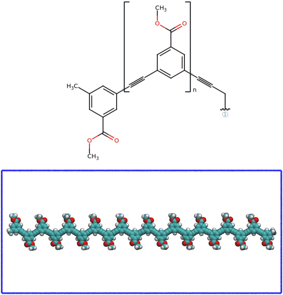

Fig. 1 (top) Chemical structure of the meta-substituted methylbenzoate phenylacetylene monomeric unit. (bottom) Structureless elongated random coil view of the starting poly-phenylacetylene (pPA) foldamer considered in this work. The structure was drawn with OpenBabel online tool.¹⁹ The simulations were performed for three values of n: n = 12 dodecamer 12mer-; n = 16 hexadecamer 16mer- and n = 20 eicosamer 20mer- polymers. This latter is shown as case-illustration example.

The simulations were performed in three different solvents with different polarities, n-hexane (nC₆H₁₄), cyclohexane (cC₆H₁₂) and water (H₂O), listed in increasing order of polarity (see Table SI and further below, ESI†). In all cases the solvent molecules were added into a rectangular box containing the solute moiety aligned along the x-axis. The different computed systems and their corresponding unit box dimensions are shown in Table 1. While TIP3P water model²⁶ was used for simulations in aqueous milieu, a united atom representation for cyclohexane cC₆H₁₂ was prepared following our previous methodology.^8,27 Meanwhile, the topology of n-hexane nC₆H₁₄ was built as described above for the pPA-oligomer.

Table 1 Summary of simulated systems. Five different runs were performed for each system starting from the same initial conformer but using different random seed

Solvents	pPA-oligomer	Simulation box (nm^3)	#Atoms	Conc. (g L^−1)	Time (ns)
H2O	12mer	9.2 × 5.5 × 9.2	44 988	965.71	100
	16mer	10.5 × 5.5 × 10.5	58 545	969.71	100
	20mer	12.5 × 5.5 × 12.5	83 644	972.67	100
cC6H12	12mer	9.2 × 5.5 × 9.2	18 060	771.02	100
	16mer	10.5 × 5.5 × 10.5	23 526	771.07	100
	20mer	12.5 × 5.5 × 12.5	33 324	771.01	100
nC6H14	12mer	9.2 × 5.5 × 9.2	15 240	650.29	100
	16mer	10.5 × 5.5 × 10.5	19 854	620.00	100
	20mer	12.5 × 5.5 × 12.5	28 110	650.21	100

---

The final systems include atom numbers ranging from 15 240 for the smallest system size, the 12mer-pPA in n-hexane nC₆H₁₄, to 83 664 for the largest one, the 20mer-pPA in water H₂O, see Table 1. The solvent molecules were added to achieve the densities of about 970 g L⁻¹, 771 g L⁻¹, and 650 g L⁻¹ for water H₂O, cyclohexane cC₆H₁₂ and n-hexane nC₆H₁₄ respectively, roughly corresponding to the liquid phase density for each of the considered solvent at 300 K. To test for possible finite size effects and yet keep the computational effort within reasonable limits, we have also performed additional simulations for the 12mers in water (box size >2 times the original box), and for 20mers in n-hexane (box size >3 times the original box). The results are reported in ESI† Fig. SII and SSIV and confirm that finite size effects do not hamper the present findings.

Throughout the study, the atomistic molecular dynamics simulations (MD) were performed with Gromacs (version 2022.3,) molecular package.¹⁵

2.3 All-atom simulation details

The solute's potential energy of the solvated systems was minimized by relaxing the solvent around the solute atoms before running the unrestrained MD simulations. During the energy minimization stage, we employed the steepest descent minimization algorithm with a minimization step size of 0.01 nm and a maximum convergence force of 500.0 kJ mol⁻¹ nm⁻¹. Thereafter, an equilibration round in the canonical NVT ensemble was performed for 5 ns using the accurate leap-frog stochastic dynamics integrator with a simulation time step of 1 fs. While long-range electrostatics interactions were accounted with the particle mesh Ewald summation, short-range electrostatics and van der Waals interactions were truncated with a single-range cutoff at 12 Å with the pair list updated every 20 steps. The velocity for the Maxwell distribution temperature was set to 300 K. The temperature of the full system was equilibrated to this latter reference value using the velocity rescaling (modified Berendsen thermostat)²⁸ with a coupling constant of 0.1 ps. To mimic the density of the realistic bulk-like phase, all the simulations were replicated in the 3D space using periodic boundary conditions and all bonds involving hydrogen atoms were restrained using LINCS algorithms.²⁹

The second equilibration run lasts 5 ns and was performed in the isobaric–isothermal NPT ensemble using the same parameters as described above for NVT. Moreover, the pressure was kept around the reference value of 1 bar using the Parrinello–Rahman pressure coupling³⁰ with a coupling constant of 1.0 ps. In the final production stage, the restrains on heavy atoms were released and the systems evolved for 100 ns without imposing any constraints on solutes bending and dihedral degrees of freedom, see Table 1.

To improve the sampling statistics, five independent runs were submitted starting from the same initial structure, but using different random seed generators.

In this description, the total potential energy of the system is given by

In eqn (4), the first four components are bonded potentials that describe bonds, angles, proper dihedrals and improper torsions of the covalent structure, respectively. The last two terms run over all pairwise atoms i and j separated from each other by a distance r_ij = |r_j − r_i| and showcase the nonbonded interactions. The bond stretching and bond bending (1st and 2nd terms in eqn (4)) model the energetic change accompanying the deformations of the bond lengths l and bond angles Θ from their respective equilibrium values l₀ and Θ₀. These two interactions are mainly computed using a harmonic-like potential with force constants k_r and k_Θ. The third and fourth terms in eqn (4) account for bond rotations. Here k_ψ is the height of the rotational barrier associated to the proper dihedral angle ψ characterized by the torsional angle phase ϒ for each Fourier component n (periodicity). Improper torsions ensure planarity in aromatic rings and allow distinguishing molecules from their mirror images in which k_ω is the force constant for the improper dihedral ω going up and down its equilibrium position ω₀. The last two components of eqn (4) describe the van der Waals repulsive (at short distance, r⁻¹² term) and attractive (at long distance, r⁻⁶ term) pairwise atomic forces between i and j shown as Lennard-Jones 12-6 potential, and the electrostatic interactions. The variables q_i and q_j are the partial charges on pairwise atoms i and j separated by the distance r_ij, σ_ij is the distance at which the Lennard-Jones potential is zero and ε_ij is the well depth.

2.4 Potentials of mean force (PMF)

In order to scrutinize the interaction modes when two cyclohexane cC₆H₁₂ or n-hexane nC₆H₁₄ entities approach each other, thereby characterizing the extent of their hydrophobicity, we computed the potential of mean force (PMF), W(r) of each of these moieties. The set-up employed follows the methodology described by Sarma and Paul^31,32 in which a system comprising 10 molecules of each type, parameterized in a united-atom like model representation, were randomly inserted into a cubic box of 15.24 nm³ volume. Subsequently, 490 TIP3P water solvents were added to fill the simulation box, leading to an overall 500 molecules for each starting system, corresponding to a concentration of about 1.089 M (∼0.013 g L⁻¹). After a preliminary steepest descent minimization, one round of NPT equilibration with position restrains was performed for 10 ns using the Parrinello–Rahman pressure coupling (τP = 0.5 ps). This run ensures a mechanical equilibration while the volume is fluctuating. The final box volume corresponding to the pressure of 1.01325 bar is then stabilized at the end of the simulation and used in the forthcoming runs. Thereafter, while still keeping the solute's atoms frozen, we performed a short NVT equilibration for 10 ns using the velocity rescaling thermostat (τT = 0.1 ps) thereby maintaining the temperature around 298.15 K. Finally, fully unrestrained MD runs in canonical NVT were performed for 100 ns and the frames were saved every 25 ps. In all the simulations, a time-step of 10⁻¹⁵ s was used.

The Lennard-Jones parameters σ_ij and ε_ij for two interacting sites i and j were obtained by employing the Lorentz–Berthelot combining rules σ_ij = (σ_i + σ_j)/2 and . Those values were taken equal to 0.3497 nm and 0.7266 KJ mol⁻¹ for –CH₂– in cyclohexane cC₆H₁₂,³³ whereas the corresponding values for n-butane as previously reported by Jorgensen et al.³⁴ were used for nC₆H₁₄: 0.3905 nm and 0.7322 KJ mol⁻¹ for sp³-methyl group, and 0.3905 nm and 0.4937 KJ mol⁻¹ for sp³-methylene building units. Moreover, long-range electrostatics interactions were computed with the particle mesh Ewald scheme, while short-range electrostatics and van der Waals interactions were truncated with a single-range cutoff at 12.2 Å with the pair list updated every 10 steps.

The pair radial distribution functions g(r) were computed for each of the molecular pairs involved, i.e. cC₆H₁₂–cC₆H₁₂ or nC₆H₁₄–nC₆H₁₄, cC₆H₁₂–H₂O or nC₆H₁₄–H₂O, and H₂O–H₂O. Subsequently, the PMF, W(r) was computed using the relation

W(r) = −k_BT ln g(r) (5)

where k_BT ≈ 0.593 KJ mol⁻¹ at T = 298.15 K.

2.5 Solvation free energy

The solvation free energy ΔG_s can be defined as the difference between the free energy of a solute in a specified solvent G_s and in vacuum G₀

ΔG_s = G_s − G₀ (6)

If ΔG_s < 0 the process is spontaneous indicating that solvation is favored. This concept can clearly be extended to the free energy transfer from solvent s₁ to solvent s₂

ΔΔG_s1>s2 = ΔG_s1 − ΔG_s2 (7)

From the numerical viewpoint, free energy differences can be conveniently computed by using thermodynamic integration⁶

where V(r,λ) is the potential energy of the system as a function of the coordinate vector r, and 0 ≤ λ ≤ 1 is a switching-on parameter allowing a gradual change from state λ = 0, where the solute is fully interacting, to state λ = 1 where it does not interact at all. The average 〈…〉_λ in eqn (8) is the usual thermal average with potential V(r,λ) = (1 − λ)V(r,0) + λV(r,1) at a fixed value of λ. The λ interval [0,1] is partitioned into a grid of small intervals, molecular dynamics simulations are performed for each value of λ belonging to each interval, and the results are then integrated over all values of λ to obtain the final free energy difference. In the present study, 21 lambda points for each simulated system were used.

The solvation free energy was computed for each of the three polymer sizes in both solvents considered here at the temperature of 300 K. Following our previous protocol,^8,27 we kept the polymers stretched, thereby maximizing the number of solute–solvent contacts, by applying harmonic restrains at the meta-substituted sp³-methyl carbon atom end-points. Moreover, cyclohexane cC₆H₁₂ and n-hexane nC₆H₁₄ were both modelled in their united atoms conformations while for water H₂O molecules the TIP3P model was employed. A simulation time step of 1 fs (for cC₆H₁₂) or 2 fs (for nC₆H₁₄ and H₂O) was generally used, depending on the relative stability of the system. The accurate leap-frog stochastic dynamics integrator was applied in all the simulations, with the Berendsen coupling pressure scheme for simulations in cC₆H₁₂ and Parrinello–Rahman analog for those in nC₆H₁₄ and H₂O.

Performing this calculation for different temperatures, allows to single out the separate contribution of the solvation enthalpy ΔH_s and the entropy ΔS_s as in ref. 8 and 27.

3 Results and discussion

3.1 Bead-spring polymer in a Lennard-Jones liquid

We start our discussion by investigating the conformational changes of a single polymer chain, represented by a Kremer–Grest bead-spring model¹² in a solvent formed by spheres interacting via a Lennard-Jones soft potential. The quality of the solvent is regulated via the ratio ε_ms/ε of the monomer–solvent attraction ε_ms and the monomer–monomer and solvent–solvent attraction ε assumed to be equal. Hence, ε_ms/ε < 1 represents a poor solvent, ε_ms/ε > 1 a good solvent, and ε_ms/ε = 1 a neutral (θ) solvent. In this latter case, the conformational properties of the chain depends on the temperature only, whereas in good and poor solvents, they depend on both solvent quality and temperature.

A detailed analysis of this paradigmatic system has already been carried out recently by Huang and Cheng.¹³ Here we follow closely their approach, reproduce the part of their analysis that is of interest for the present study, and include an additional case that was not considered in ref. 13. Fig. 2 depicts the collapsed conformation of the chain under (a) poor solvent condition ε_ms/ε = 0.2, (b) neutral condition ε_ms/ε = 1.0, and (c) good solvent condition ε_ms/ε = 4.0. While in the first two cases, the results follow the expected behaviour of collapsing in poor solvent and of remaining swollen in neutral solvent, in the last case ε_ms/ε = 4.0 of strong monomer–solvent attraction, the chain is observed to undergo a collapse, albeit with a qualitatively different folded conformation compared to the poor solvent condition of case (a). The authors of ref. 13 ascribed this second collapse to a bridging mechanism occurring above a certain strength of the monomer–solvent attraction, where an effective monomer–monomer attraction sets in mediated by the solvent, mirroring a similar effect occurring in colloids.³⁵ As the attraction increases from poor solvent (ε_ms/ε = 0.2), the radius of gyration R_g (a standard order parameter for the onset of the coil-globule transition) is observed to increase at the onset of the neutral ambient (ε_ms/ε = 1), to remain swollen with large R_g until (ε_ms/ε ≈ 2.5) and to collapse again above this value. In ref. 13 it was explicitly checked that both phases are collapsed phases with the correct R_g ≈ N^1/3 behaviour. In this second folded conformation, however, some solvent molecules remains inside the polymer globule and induce an effective monomer–monomer attraction. This, along with the gain in solvent entropy achieved upon folding, stabilizes this folded conformation against the coil counterpart. All simulations started with a preliminary equilibration of 4.0 × 10⁶τ with the equilibrated solvent at a density of about 0.64m/σ³.¹³ To avoid possible surface effects, the number of solvent beads was adjusted so that the size of the cubic box was sufficiently larger than the radius of gyration.

Fig. 2 Snapshot of equilibrated configuration of a Kremer–Grest bead-spring polymer in a Lennard-Jones solvent at constant temperature T* = k_BT/ε = 1 and different monomer–solvent interactions: (a) ε_ms/ε = 0.2; (b) ε_ms/ε = 1.0; (c) ε_ms/ε = 4.0. Same as above but when the monomer–solvent interactions is ε_ms/ε = 1.0 and for decreasing temperatures: (d) T* = 2.0; (e) T* = 1.0; (f) T* = 0.1. The condensation effect of the solvent in the latter case is particularly noteworthy. Cases (b) and (e) are statistically equivalent. The size of the solvent, nominally identical to the polymer bead, has been artificially reduced for clarity.

Interestingly, the same re-entrant behaviour is not observed in the case where a polymer collapses in a neutral solvent (ε_ms/ε = 1) upon cooling the temperature. This case was not analyzed in ref. 13 and its reported here in Fig. 2d–f, where we see that a chain originally swollen at T* = 2.0 (Fig. 2d) becomes slightly more compact under θ condition T* = 1.0, and eventually collapses into a globule upon further cooling at T* = 0.1. A quantitative measure of these conformational changes can be obtained from the radius of gyration R_g. Fig. 3 (top panel) depicts the reduced radius of gyration R_g/σ as a function of ε_ms/ε, a measure of the solvent quality, from the simulations with N = 128 monomers. Here the reduced temperature is T* = 1 corresponding to room temperature, and this is the same case whose snapshots are reported in Fig. 2. At low ε_ms/ε (poor solvent regime) the polymer is collapsed and R_g/σ is very small. Upon approaching ε_ms/ε = 1 (neutral solvent regime), R_g/σ starts to increase until reaching a maximum of R_g/σ ≈ 9 at ε_ms/ε = 1.4 (good solvent regime). A further increase of ε_ms/ε leads to a marked decrease of R_g/σ that is to be associated to a re-entrant collapse mediated by the solvent, as anticipated. Although, the details of the calculation are slightly different, these results exactly reproduce the findings of ref. 13, supporting the robustness of this water-bridging interpretation. Fig. 3 (bottom panel) reports the same calculation in which the solvent quality is kept fixed at neutral condition ε_ms/ε = 1, and temperature is reduced. Unlike previous case, clearly we observe a single coil-globule transition as a function of the (reduced) temperature T*. It is important to remark that the solvent itself tends to collapse upon cooling (see Fig. 2f), and this explains the difference between this results and the textbook results from simulations in implicit solvents that show a much more marked transition. While it is rewarding to observe a consistent picture stemming from different calculations, this example highlights how the equivalence decreasing the temperature = decreasing the solvent quality must be taken with great care, even in this very simple and paradigmatic example. Indeed, the actual phase diagram for this problem has been further shown to be even richer.³⁶

Fig. 3 (top) Radius of gyration R_g (in units of σ) as a function of ε_ms/ε in the case of N = 128 monomers. In this case T* = 1 corresponding to room temperature; (bottom) radius of gyration R_g (in units of σ) as a function of the reduced temperature T* again for N = 128. In this case ε_ms/ε = 1 corresponding to “neutral” (θ) solvent. Error bars are displayed as vertical bars centered in each point.

3.2 Potential of mean force of cyclohexane cC₆H₁₂ and n-hexane nC₆H₁₄ in water

The analysis of previous section clearly shows that the conventional paradigm of good/poor solvent falls short in describing even a simple bead-spring model in a Lennard-Jones solvent. Consider now a real polymer in a real solvent, both of which will then be described atomistically. A polymer is customarily described in terms of structural units (the monomers) that are chemical moieties that can be either polar or hydrophobic. Likewise, the solvent can be either polar or hydrophobic or something in between. Strictly speaking, a polar molecule has a permanent dipole (hence the name), whereas a hydrophobic molecule has not. However, for a more complex chemical moiety – in particular for a solvent, this distinction become fuzzy and one frequently used quantification of the polarity of the solvent is via the relative dielectric constant. Accordingly, a solvent is polar if the relative dielectric constant is high, hydrophobic if the relative dielectric constant is low. Three different solvents are considered in the present study. Water H₂O is highly polar with a relative dielectric constant 80.1. While liquid water anomalies still defy a complete description,³⁷ the geometry of the molecule is very simple with a typical length scale of approximately 1.5 Å and a H–O–H angle of ≈106° (Fig. 4). At the opposite side of the scale, there are the organic solvents with low relative dielectric constant. Cyclohexane cC₆H₁₂ has relative dielectric constant 2.02, a typical size of 5 Å, and is formed by a nearly flat single a 6-vertex aromatic ring (Fig. 4). Similarly, n-hexane nC₆H₁₄ is a straight-chain alkane with 6 carbon atoms with a characteristic size of 6 Å (Fig. 4) and it has a relative dielectric constant 1.88. For comparison, Fig. 4 also includes acetonitrile MeCN (dielectric constant 37.5) and chloroform CHCl₃ (dielectric constant 4.81) as polar and hydrophobic solvents already used in this framework.³⁸ Hence, Fig. 4 is ordered according to the dielectric constants on the horizontal axis and according to the characteristic size l on the vertical axis.

Fig. 4 Characteristic sizes l (vertical axis) of the considered solvents as a function of their polarities (horizontal axis). From left to right the overall size of water H₂O (1.515 Å), chloroform CHCl₃ (2.56 Å), acetonitrile MeCN (3.00 Å), cyclohexane cC₆H₁₂ (5.80 Å) and n-hexane nC₆H₁₄ (6.34 Å), respectively. The length of water is easily computed from the O–H bond stretching (∼0.943 Å) and H–O–H bending angle (∼106°). The length of cyclohexane is obtained from the work of Fomin and coworkers,³⁹ and that of n-hexane estimated from Boese et al.⁴⁰ Other data from ref. 41.

Following Smith and Haymet,⁴² we performed molecular dynamic simulations of both cyclohexane cC₆H₁₂ and n-hexane nC₆H₁₄ in water to illustrate the hydrophobic effect, that is the tendency of hydrophobic solutes to aggregate to avoid unfavourable contacts with water.⁷Fig. 5 reports the final configuration of 10 cyclohexane cC₆H₁₂ molecules (left panel) and 10 n-hexane nC₆H₁₄ moecules (right panel) in a aqueous solution formed by 490 water H₂O molecules, thus providing a visual confirmation of the tendency of both cyclohexane cC₆H₁₂ and n-hexane nC₆H₁₄ to aggregate in water H₂O. They do it differently, however. A quantitative way to assess the relative hydrophobicity of the two organic solvents cC₆H₁₂ and nC₆H₁₄ relies on the calculation the potential of mean force W(r) between the two points distant r apart in a water solution and belonging to two different molecules. In both cases we used the center-of-mass (COM) distance between pairs of molecular moieties to measure the distance r. In the case of cyclohexane cC₆H₁₂ COM is nearly coincident with the center of the aromatic ring, whereas in the case of n-hexane nC₆H₁₄ COM falls on the central carbon atom. The calculation was carried out only for non-bonded interactions. For both organic molecules there are marked oscillations between 0.1 nm and 0.4 nm distances, with considerably deep local minima indicating strong attractions between similar moieties, as expected from their hydrophobic characters. We surmise that the minimum at 0.15 nm corresponds to H–H stacking of in the cyclohexane cC₆H₁₂ case and to the side-side alignment in the case of n-hexane nC₆H₁₄ (see Fig. 4) as also suggested by the snapshots of the final equilibrated conformations in Fig. 5. Also in both cases, the first and the second local minima are located at approximated distances 0.15 nm and 0.25 nm, somewhat closer compared to the results of Smith and Haymet⁴² who performed a similar calculation for two methane molecules and found these two minima located at 0.40 nm and 0.65 nm. The depth of the first deeper minimum (≈1 kCal per mole) is similar to that found for methane in ref. 42. Several differences are however visible between the cC₆H₁₂–cC₆H₁₂ interactions (solid magenta line) and the nC₆H₁₄–nC₆H₁₄ interactions (solid blue line). In the case of cC₆H₁₂–cC₆H₁₂ interactions (solid magenta line) both the minima and the maxima are rather narrow and deep compared to those of nC₆H₁₄–nC₆H₁₄ interactions that are much broader (solid blue line). Also the first large and positive energy barrier occurs around 0.075 nm for nC₆H₁₄–nC₆H₁₄ interactions (solid blue line) and around 0.13 nm for cC₆H₁₂–cC₆H₁₂. Finally, cC₆H₁₂–cC₆H₁₂ interactions (solid magenta line) present a third minima which is absent in the nC₆H₁₄–nC₆H₁₄ counterpart.

Fig. 5 Snapshots of equilibrated cyclohexane cC₆H₁₂ in water H₂O (left) and n-hexane nC₆H₁₄ in water H₂O (right). Hydrogen bonds forming network between solvent entities are explicitly displayed.

Fig. 6 Potentials of mean force of cyclohexane cC₆H₁₂ (magenta solid line) and of n-hexane nC₆H₁₄ (blue line) molecules in water H₂O solvent. The corresponding radial distribution functions are shown in ESI† Fig. SI. The considered moieties are the center of the aromatic ring for cyclohexane and the central carbon for n-hexane (see text). Only non-bonded interactions were considered.

These findings are consistent with the idea that the two solvents are expected to interact similarly with water, having very similar chemical properties – the nearly identical dielectric constants, and very similar geometric sizes (as represented by the diameter of the equivalent van der Waals sphere), but not identically. As cyclohexane cC₆H₁₂ and n-hexane nC₆H₁₄ have different shapes, as displayed in Fig. 4, this might induce a difference in their solvation entropies that will be discussed further below.

3.3 Characterization of the folding process of poly-phenylacetylene (pPA)

Let us recapitulate our previous findings and put them in the perspective of the next step. Consider the work by Vasilevskaya et al.⁴³ who studied the conformational equilibrium properties of amphiphilic polymers in a poor solvent. The amphiphilic polymer was modelled by a chain of hydrophobic monomers (H-type) with a side-chain polar group (P-type), and the poor solvent character was modelled implicitly by modulating the H–H, H–P, and P–P interactions. At constant (room) temperatures, a collapse of the chain was achieved by favouring the H–H and P–P interactions with respect to the H–P ones. This promotes segregation of the H and P groups and hence it induces the collapse of the chain. Now imagine extending this study to explicit solvent, as it was done in the bead-spring model. This requires the additional classification of the solvent in hydrophobic (H-type) or polar (P-type). The collapse of the amphiphilic polymer will then be promoted by a P-type (H-type) solvent if monomer character is mainly hydrophobic (polar). In the case of a perfect H–P amphiphilic polymer containing an identical numbers of hydrophobic and polar groups, both H and P-type of solvent will be neutral and the coil-globule transition can occur only upon cooling.

Poly-phenylacetylene (pPA) (Fig. 1) is a nonbiological polymer that belongs to the general class of aromatic foldamers^44,45 that are of considerable interest for its potential technological applications.⁴⁶ A key observation was that pPA chain adopts a nonflat helical structure,^9,38,47–52 and this opens many perspectives associated with its helicity. It is a polymer formed by repeated units of an alkyne hydrocarbon containing a phenyl ring (the monomers) whose rigidity promotes the helical shape upon folding,⁵³ whose shape, chirality, and self-assembly properties are the result of a delicate balance between the various interactions, and modification of the solvent polarity and/or the temperature may promote some factors over the others, and hence affect this delicate balance. A deeper understanding of these factors is the main driving force for the present study that builds on important past contributions. Nelson et al.⁹ first observed that pPA m-th oligomers (with m ≥ 7) undergoes a coil-helix transition in a putative poor solvent such as chloroform CHCl₃ (see Fig. 4). Upon replacing the benzoate side chain CH₃ (Fig. 1) with hydrogen H, the folding occurs in water H₂O, so in this case also water acts as a poor solvent for pPA. The same backbone but with a slightly different side chain was used in a latter study by the same group³⁸ and it was found that it remains in a random swollen conformation in a putative good solvent such as acetonitrile MeCN (see Fig. 4). The kinetic of the process has also been studied both experimentally⁴⁹ and numerically⁵⁰ again for an oligomer different from that considered in the present study (Fig. 1). Two key aspects remaining unclear from these studies are a clear understanding of the driving force for collapse, and a clear definition of “good” and “poor” solvent for pPA. One preliminary step in this direction was performed by Sen⁵¹ in the case of H side chain, but this study was unable to investigate the full folding process because of it high computational cost out of reach at that time. To the best of our knowledge, the present study is hence the first full-fledged atomistic investigation of this particular oligomer that can be compared with the experiments of ref. 9. The present study will further offer several additional insights stemming from the use of different solvents.

MD atomistic simulations of a single chain of poly-phenylacetylene (pPA) (with CH₃ side chain, see Fig. 1) with different number m of monomers, from 12 to 20, in solvent of different polarities were performed according to the aforementioned prescription. As anticipated, we choose to represent the polarity of a solvent by its (relative) dielectric constant (see Fig. 4). Hence, solvents ranging from polar (water H₂O) to hydrophobic (cyclohexane cC₆H₁₂ and n-hexane nC₆H₁₄), were employed. With reference to past work, we note that in this classification, choloroform CHCl₃ (dielectric constant 4.81) is hydrophobic, whereas acetonitrile MeCN (dielectric constant 37.5) is polar. As pPA (with CH₃ side chain) is predominantly hydrophobic in character due to its chemical structure (see Fig. 1), one might expect a random coil conformation in a hydrophobic solvent such as cyclohexane CC₆H₁₂, and a folded helical conformation in a polar solvent such as water H₂O. Note, however, that this expectation is already not consistent with experimental findings of Nelson et al.⁹ who observed the folding of the chain in chloroform CHCl₃ hydrophobic in our classification (dielectric constant 4.81). In all cases, the system was kept at room temperature. As it will be further elaborated below, the temperature may also be expected to play an important role. For example a polystyrene (predominantly hydrophobic) single chain was observed to collapse in cyclohexane (also hydrophobic) upon cooling from 35.0 °C to 28 °C.⁵⁴

Our results are reported in Fig. 7, where the root-mean-square-deviation from the initial stretched conformation (depicted in the far left inset of the figure) is displayed during the time evolution of the system in the case where pPA is dispersed in water H₂O (red curve), cyclohexane cC₆H₁₂ (black curve) and n-hexane nC₆H₁₄ (green curve). Three different number of monomers (n = 12, n = 16, n = 20) are reported from top to bottom to test for the length dependence. Representative snapshots of the different conformations of the pPA polymer are also displayed in Fig. 7 as insets, color coded according to the relative curve. It is apparent how, for all three solvents and chain lengths, the RSMD displays an initial increase eventually reaching a plateau thus indicating the tendency to form a final globular conformation different from the initial extended conformation. However, while in water the conformational transition appears to be rather stable after a transient period of about 20 ns, both in cyclohexane and (to a less extent) n-hexane the chain appears to fold/unfold erratically, thus suggesting that the folded state is not fully stable at this temperature in both solvents. These results also appear to be independent on the length of the polymer, the three panels of Fig. 7 being very similar to one another. In the experiments reported in ref. 9 and 38, acetonitrile MeCN (dielectric constant 37.5) was used as polar solvent, whereas cholorophorm CHCl₃ (dielectric constant 4.81) was used as nonpolar (hydrophobic) solvent. Our findings appear to be consistent with theirs, as they found a stable fold for octamers or above only in acetonitrile (polar), whereas no folding was observed in cholorophorm (hydrophobic). Yang et al.⁴⁹ also reported experimental folding of pPA dodecamer in 50/50 THF/methanol, and Elmer and Pande⁵² performed detailed numerical simulations and unconvered kinetic trapping occurring during the folding pathway. A glance to the most representative snapshots reported in ESI† Fig. SIX shows how within each helical structure (either stable or unstable), the highly charged oxygen atom of each monomer tends to avoid a close contact with the oxygen atoms of the non-bonded neighboring monomers to minimize the high repulsive energy, although this is partially mitigated by the presence of the hydrogen atoms within the same monomers. This was noted before.¹⁰ Although this prevents the achievement of a perfect π–π stacking between consecutive rings, the next analysis shows that in water this turns out not to be a crucial feature. Additional insights can be obtained by accumulating the pseudo-bond length b (i.e. the effective distance between monomers, also known as Kuhn length³), the bending angle θ between three consecutive i − 1, i, and i + 1 monomers, and the dihedral angle μ, the angle between two consecutive planes involving the i − 1, i, i + 1, and i + 2 monomers as shown in Fig. 8a,⁵⁵ and whose distributions along the equilibrated trajectory is reported in Fig. 8b–d. Here, the representative point of the monomer is the geometrical center of its phenyl ring, see the top panel of Fig. 1. Coherently with previous findings, the distribution of the pseudo-bond lengths in water H₂O is peaked around 6.85 Å, with that in both cyclohexane cC₆H₁₂ and n-hexane nC₆H₁₄ both peaked at a slightly larger value (Fig. 8a). A more significant difference is observed for the bending angle θ whose distribution is found to centered at θ ≈ 115° in water and at θ ≈ 118° in both cyclohexane and n-hexane (Fig. 8c). An even more marked difference is finally observed for the distribution of the dihedral angles μ whose distribution is found to be centered at μ ≈ −10° in water, indicating a stable π–π stacking of the consecutive phenyl rings thus eventually leading to the helical structure (red curve Fig. 8d bottom panel). By contrast, both cyclohexane and n-hexane display additional peaks in the dihedral angle μ close to μ ≈ ±180° indicating that the fold/unfold dynamical process occurs with a high frequency even after the equilibration has been achieved, in agreement with the results of Fig. 7. As in the study by Nelson et al.,⁹ in all cases the collapsed structures were found to be helices as reported in ESI† Fig. SX. As mentioned, this is to be ascribed to the rigidity of the aromatic chain forming the chain backbone, which forces the chain to fold into a helicoidal structure via π–π stacking, and it is fully formed only when the chain length (that is the number of monomers) is sufficiently long and commensurate with the pitch of the chain.

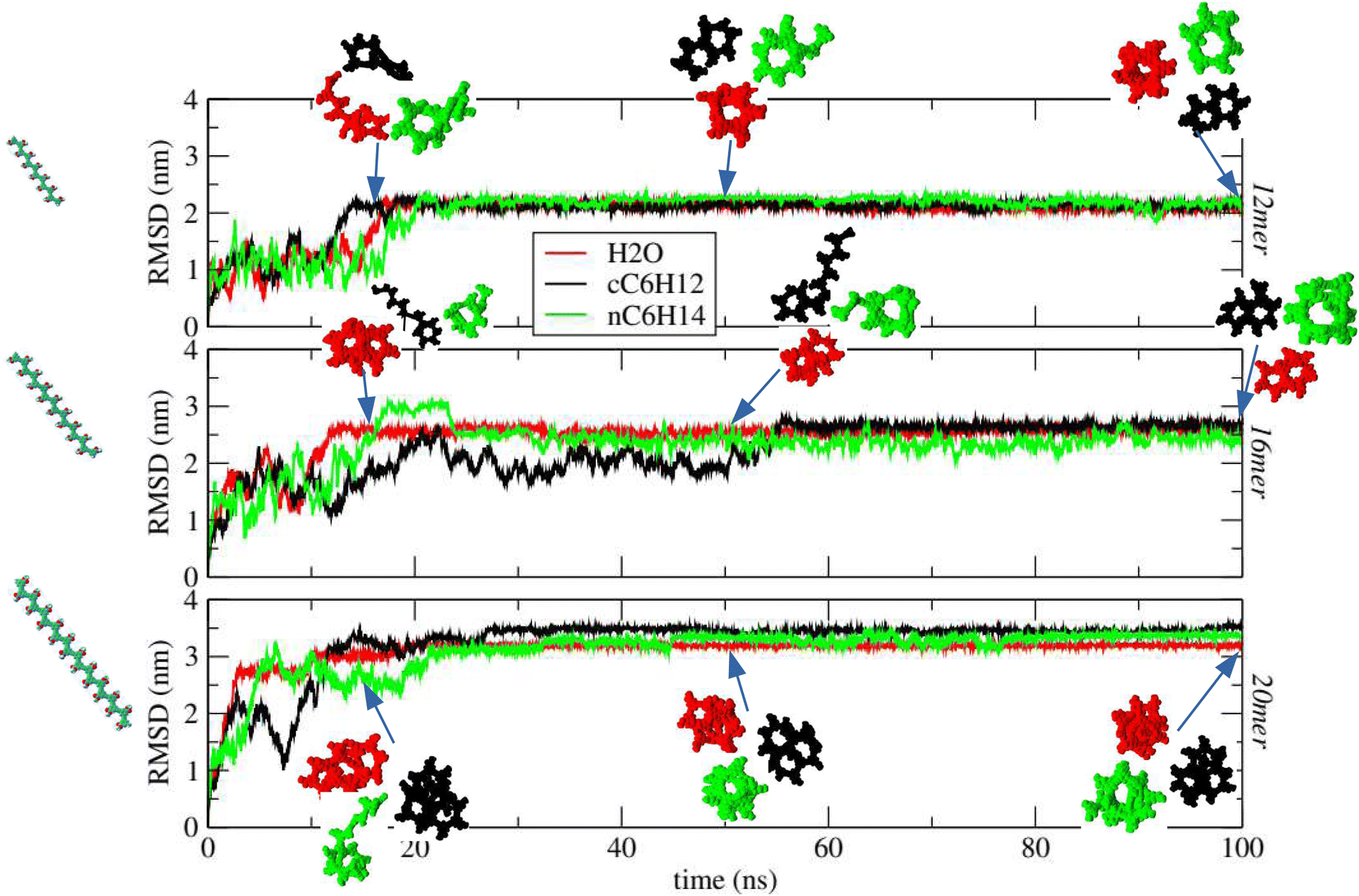Fig. 7 Root-mean-square-deviation (RMSD) from the initial conformation along the selected simulation trajectories. All the simulations started from the extended swollen conformations (left most inset view) and representative snapshots are extracted at representative time frames 15, 50, and 100 ns. Simulations performed in water H₂O (red curve), cyclohexane cC₆H₁₂ (black curve), and n-hexane nC₆H₁₄ (green curve) have also insets displaying representative snapshots with the same color code. From top to bottom results are reported for oligomer lengths 12mer, 16mer and 20mer.

Fig. 8 (a) Definitions of the pseudo-bond (Kuhn) length b, bond bending angle θ, and dihedral angle μ;⁵⁵ (b) distribution of the pseudo-bond length b; (c) distribution of bond bending angle θ; (d) distribution of the dihedral angle μ. Results include different oligomer units 12mer, 16mer and 20mer, and different curves refer to the three different solvents, water H₂O (red), cyclohexane cC₆H₁₂ (magenta) and n-hexane nC₆H₁₄ (cyan) employed in this work.

Additional insights can be obtained by computing the intramolecular site–site pair radial distrubution function between carbon atoms of pPA methoxycarbonyl group in the three solvents. This is reported in ESI† Fig. SV and displays clear peaks approximately 0.5 nm apart in water and n-hexane, a value that matches rather well with the distance between the aromatic planes in the π–π stacking.⁵⁶ By contrast, in cyclohexane, the peak distribution is fuzzier coherently with an unstable fold.

Within the common paradigm of good and poor solvent outlined in the paradigmatic case of a bead-spring polymer in a Lennard-Jones fluid, the above findings can be interpreted in terms of a polymer backbone mainly hydrophobic that collapses in water environment but not in an organic hydrophobic solvent such as cyclohexane or n-hexane. This is also consistent with another study⁵⁷ where MD simulations of a single carboxylate-substituted poly para phenylene ethynylene (PPE) chain in different solvents (water H₂O and toluene C₆H₅CH₃) were performed. In that case too, the chain was found to remain extended at room temperature in toluene, and found to collapse in water.

The results of Fig. 7 appears to have only a minimal dependence on the length of the polymer, with nearly identical behaviour in the case of oligomer lengths 12mer, 16mer and 20mer. This was to be expected. Nelson et al.⁹ observed experimental folding of a phenylacetylene oligomer only for oligomer length 6 or above, with the rigid nature of the phenyl ring preventing π–π stacking for too short chains. Likewise Prince et al.³⁸ observed the collapse of the chain in acetonitrile (polar) for oligomer length 8 or above. As all oligomer lengths reported in Fig. 7 are in all cases sufficiently long to allow π–π stacking, it is not surprising that the results turn out to be independent of the lengths.

3.4 Additional quantitative probes of the folding process

To provide additional evidence of the folding process, we also monitored the the radius of gyration (m_i is the mass of the i-th atom, R_CM is the center of mass of the polymer chain, and M is the total mass), and the solvent accessible surface area (SASA) using the algorithm devised by Eisenhaber et al.⁵⁸ We note that SASA can be regarded as a proxy of the sum of the cavity and van der Waals contributions to the solvation free energy⁶ and hence its monitoring is particularly insightful. For five independent runs, the average 〈R_g〉 and the standard deviation are reported in Fig. 9 (left). Three different number of monomers n = 12, 16, 20 were considered for all three different solvents. The same quantity is also plotted as a function of the number of monomers n in Fig. 9 (right), to identify the various phases. We find that 〈R_g〉 ≈ n^ν with ν ≈ 0.29 for water H₂O, in reasonable agreement with the value ν = 1/3 expected for the collapsed phase; ν ≈ 0.49 in the case of cyclohexane cC₆H₁₂, and ν ≈ 0.47 in the case of n-hexane nC₆H₁₄, both somewhat lower of the Flory value ν = 3/5 expected for the swollen phase in a good solvent,^1,2 likely indicative of the aforementioned erratic folding/unfolding process. It is here worth recalling that, strictly speaking, the above scaling laws are only valid in the thermodynamic limit, that is for sufficiently long polymers,² and hence a deviation from these laws is to be expected for short oligomers such as those discussed here.

Fig. 9 (left) Average pPA radius of gyration 〈R_g〉 for the individual runs performed. The error bars represent the standard deviations. All the three solvents water H₂O, cyclohexane cC₆H₁₂, and n-hexane nC₆H₁₄ are displayed for each of the oligomer's length 12mer, 16mer and 20mer considered here. The related time-based plots are shown in ESI† Fig. SII, SSIII, and SSIV. (right) Average pPA radius of gyration versus the number of monomers n for the three different solvents water H₂O, cyclohexane cC₆H₁₂, n-hexane nC₆H₁₄. Fitted slopes are also reported in the three cases. These results were obtained at room temperature of 300 K.

The results of Fig. 9 were obtained at room temperature of 298.15 K. However, the folding process appears rather stable against a temperature change in the interval 270–330 K, which brackets the 298.15 K temperature and coincides with thar previously used for oligopeptides.⁸ This is shown in Fig. 10 where the average radius of gyration 〈R_g〉 is reported at a function of the temperature T in the temperature range 270–330 K. Although we eventually expect to have a marked collapse of the chain for sufficiently low temperatures for all three solvents, the apparent insensitivity in this temperature range is rather intriguing.

Fig. 10 Temperature dependence of the average pPA radius of gyration for different oligomer length (a) 12mer, (b) 16mer and (c) 20mer in the three solvents water H₂O, cyclohexane cC₆H₁₂, and n-hexane nC₆H₁₄ considered here. (d) Average pPA accessible surface area over the independent simulations performed at 300 K temperature. The error bars stand for standard deviations. All the three solvents water H₂O, cyclohexane cC₆H₁₂, and n-hexane nC₆H₁₄ are displayed along with the oligomer's length 12mer, 16mer and 20mer used in this work. The corresponding time-based plots are shown in ESI† Fig. SII, SSIII, and SSIV.

The analysis of SASA at 298.15 K temperature provides consistent results. This is reported in Fig. 10d where SASA values are displayed for same three different number of monomers n and for the three different solvents: water H₂O, cyclohexane cC₆H₁₂, and n-hexane nC₆H₁₄. For all different n, SASA in water shows consistently lower values compared to both cyclohexane and n-hexane, indicative of a more stable collapsed phase, in agreement with the results of Fig. 7 and 9.

A final conclusion can be drawn for the occurring diffusion process of the folded structures. As the collapse (when present) is from a coil to a helical-like structure, rather than a globule, the diffusion need not be isotropic. Indeed, by recording the mean square displacements (MSD) with respect to the original conformation 〈(R_GC(t) − R_GC(0))²〉 = 6Dt of the geometrical centers of 20 aromatic rings mid-points (GC) of the pPA polymer (in units of 10³ nm²) vs. time (in ns), along with the corresponding parallel 〈(R_GC,‖(t) − R_GC,‖(0))²〉 = 2D_‖t, along the helical axis direction, and perpendicular 〈(R_GC,⊥(t) − R_GC,⊥(0))²〉 = 4D_⊥t counterparts, we note that diffusion is systematically faster along the direction parallel to helical axis with respect to the direction perpendicular to it, that is D_‖ > D_⊥ > D, as it is also the case for diffusion of rigid helices.⁵⁹ Details can be found in ESI† Fig. SXIX and SSXX.

3.5 Free energy landscape

The analysis reported in previous section clearly shows how the RMSD, the average radius of gyration 〈R_g〉, and SASA can all be used as possible “reaction coordinates” to track down and assess the folding/unfolding process. Accordingly, we can construct the relative energy landscape by monitoring their joint probability distribution, and then the relative free energy landscape by using eqn (5). Following a common choice in the literature, we selected 〈R_g〉 and the RMSD as reaction coordinates and compute the free energy landscape for all the three solvents and different number of monomers. Different combinations involving also SASA provide essentially identical results (see ESI†).

Fig. 11 reports the results of this free energy landscape analysis, with the first row corresponding to water H₂O, the second row to cyclohexane cC₆H₁₂, and the third row to n-hexane nC₆H₁₄. For each row, different columns refer to different lengths of the polymer, n = 12 on the left, n = 16 in the center, and n = 20 on the right. The color code of the contour plots is reported on the right vertical bar and it goes from a shallow minimum (red) to a deep one (blue).

Fig. 11 Free energy landscape (FEL) for each of the oligomers used here and in different solvents, using the average radius of gyration 〈R_g〉 and the RMSD as reaction coordinates. From top to bottom the FEL in water H₂O, cyclohexane cC₆H₁₂ and n-hexane nC₆H₁₄ are reported for increasing number of monomers from left to right (12mer, 16mer and 20mer). The remaining FEL for all the simulations performed are reported in ESI† Fig. SSXI, SSXII, and SSXIII. Color coding for the depth of the minima is reported on the right vertical bar.

In water H₂O (first row in Fig. 11 for n = 12, n = 16, and n = 20 from left to right), a development of a well defined and stable minimum occurring at low 〈R_g〉 and high RMSD is observed upon increasing the polymer length n, clearly associated with a folded conformation. A less pronounced effect is seen in the case of n-hexane nC₆H₁₄ (third row in Fig. 11 for n = 12, n = 16, and n = 20 from left to right), with the depth of the minima much less marked. By contrast, in ciclohexane cC₆H₁₂ (second row in Fig. 11 for n = 12, n = 16, and n = 20 from left to right) we see evidence of two marginally stable minima, one corresponding to the collapsed phase as in water and the other to the extended phase, indicating the presence of frequent folding/unfolding events, in agreement with the results reported in previous sections.

Taken together, the above results indicate that at room temperature a pPA oligomer tend to have a stable collapse water H₂O, an unstable conformation with erratic folding/unfolding events in cyclohexane cC₆H₁₂, and something in between for n-hexane nC₆H₁₄, confirming the interpretation of past experimental findings.^9,38

In polypeptides, the folded state in water is stabilized also by the formation of intrachain hydrogen bonds.⁶⁰ In the case of pPA, this is not the case as discussed in the next subsection.

3.6 Intra- and inter- oligomer–water hydrogen bonds

The above findings can only partially be interpreted within the common view of “like-dissolves-like”. This limitation was noted before in surfactants with inverted polarities⁶¹ and in the case of oligopeptides.⁸ One additional interesting question is related to the hydrogen bonds that pPA forms in water H₂O – pPA obviously does not form hydrogen bonds with either cyclohexane cC₆H₁₂ or n-hexane nC₆H₁₄. In the folding process of polypeptides in water,⁸ some hydrogen bonds that the peptide chain in the original swollen conformation forms with water break down upon folding and then reform internally as a intra-chain hydrogen bonds. This is indeed a way to stabilize the characteristic secondary structure in proteins as discovered by Linus Pauling approximately 70 years ago.⁶⁰ As we will see below, this is not the case in the case of pPA.

Fig. 12 (left panel) reports the change in the number of pPA–water hydrogen bonds during the entire MD trajectory in water H₂O. The three different panels (top, middle, bottom) refers to different lengths of the pPA oligomers (12mer, 16mer and 20mer), and in all cases, the right panels depict the distribution of the hydrogen bonds. Five independent runs were performed and the colored curve displayed in Fig. 12 report the running average, whereas the underlying gray region represents the relative thermal fluctuations. Irrespective of the length of the pPA oligomer, these results unambiguously show that the total number of pPA–water hydrogen bonds does not change significantly during the folding of the pPA oligomer. Hence the optimization of the hydrogen bond distribution is not one of the driving force to fold, unlike what happens in the biopolymer case. This suggests that the main driving force for folding in water should be sought elsewhere, and this will be discussed in the next subsection.

Fig. 12 (left panel) Overview in the changes of the number of solute–solvent hydrogen bonds as a function of the simulation time in water H₂O for 5 independent runs. From top to bottom the results refer to 12mer, 16mer and 20mer respectively. The gray fluctuations represent the overlays of the simulation results while their corresponding running average are plotted in the middle. (right panel) Distribution of hydrogen-bonds during the trajectory. All the plots are on the same scale.

3.7 Non-covalent interactions

As discussed in the previous subsection, hydrogen bonds are not a stabilizing factor of the folded state and hence the question arises of what are the other potential stabilizing factors. Hydrogen bonding is present only in water but as it does not change upon folding, its contribution in the total energetic balance can be neglected altogether. Then, we next discuss the additional energetic part of the non-covalent interactions, Lennard-Jones and Coulomb interactions, that are present for all three considered solvents. Fig. 13 depicts the contribution of the Lennard-Jones interactions (Fig. 13a) contrasted with the Coulomb contribution (Fig. 13b). In both cases, different oligomer lengths have been considered. In the case of water H₂O, the Lennard-Jones contribution is negative, decreasing for increasing number of monomers. By contrast, this contribution is always positive for both cyclohexane cC₆H₁₂ and n-hexane nC₆H₁₄, larger for cyclohexane, and with no definite trend in terms of oligomer length. On the other hand, in all cases this contribution is one order of magnitude smaller than that of Coulomb interactions that is negative (that is attractive) for all three solvents. As a result, the energetic part of the non-covalent interactions is nearly identical for all three solvents and is attractive. The origin of this result is unclear. Likely, it can be ascribed to the hydrogen–oxygen interaction occurring between side chains upon π–π stacking but it remains unclear how this contribution overwhelms the repulsive oxygen–oxygen contribution. What is clear, however, is that the energetic part of the interactions cannot be invoked to explain the differences in the folding processes of pPA in the three different folding. For this reason, we are going to tackle the calculation of the solvation free energy and its separation in energetic and entropic contribution in the next section.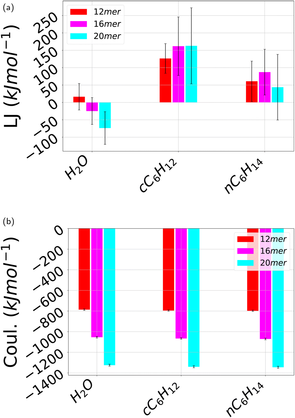

Fig. 13 Average pPA intramolecular non-covalent interaction energy over the independent simulations carried out here. (a) Lennard-Jones 12-6 interactions; (b) Coulomb interactions. The error bars stand for standard deviations. All the three solvents water H₂O, cyclohexane cC₆H₁₂, and n-hexane nC₆H₁₄ are displayed for each of the oligomer's length 12mer, 16mer and 20mer. The reference time-based plots are shown in ESI† Fig. SVI and SVII.

3.8 pPA solvation free energy

The solvation free energy can be computed via thermodynamic integration, using eqn (8). Then ΔG_solv corresponds to the difference in free energy between pPA in a gas phase and in a specific solvent. We will denote as ΔG_w, ΔG_c, and ΔG_h the solvation free energies in water H₂O, cyclohexane cC₆H₁₂, and n-hexane nC₆H₁₄, respectively. The knowledge of these three solvation free energies allows also to compute ΔΔG_w>c, and ΔΔG_w>h, that is the transfer free energy from water to either cyclohexane or n-hexane. A negative value of this quantity indicates a favorable solvation in either two solvents compared to water, the opposite for a positive value. As it also happens in the case of polypeptides,⁸ this relative quantity turns out to be the most relevant one, as it will be further discussed below.

Fig. 14a displays these free and transfer free energies, again for different oligomer lengths. While ΔG_w, ΔG_c, and ΔG_h are found to be all negative, indicating a stabilizing effect of all three solvents compared with the case of pPA in the gas phase, the relative transfer free energies turn out to be different. ΔΔG_w>c is positive and increasing with the oligomer length, whereas ΔΔG_w>h is negative, but significantly smaller in magnitude. This is a bit surprising in view of the putative predominant hydrophobicity of the pPA chain that would suggest a negative transfer free energy for both organic solvents. As the the chemical structure of the two organic solvent is nearly the same, the only alternative possibility is that the difference originates from the different shapes of the cC₆H₁₂ and nC₆H₁₄ molecules (see Fig. 4), which in turn might affect the entropic contribution to the solvation free energy. To address this possibility, we have studied the temperature dependence of the solvation free energy from which it is possible to disentangle the energetic and the entropic contributions by first computing the entropy as the derivative with respect to temperature of the free energy, and then obtaining the enthalpy as a difference (see for instance ref. 8 for details). This is done in Fig. 14b for all three solvents. The different behavior of cyclohexane cC₆H₁₂ and n-hexane nC₆H₁₄ is now clearly visible. We first note that in all three cases the slopes are negative and small. A zero slope would corresponds to the case of a process completely enthalpic dominated, a large slope to a process entropically dominated, a −1 slope to an optimal entropy–enthalpy compensation, that is what is actually occurring for polypeptides in water⁸ (see also next subsection). The results of Fig. 14b then show that the three solvation processes are all mainly enthalpically driven, but the actual energies involved are rather different, with a large enthalpy gain for both water H₂O and n-hexane nC₆H₁₄ compared to cyclohexane cC₆H₁₂. In the former case there is an entropy loss corresponding to the enthalpy gain, but with a much smaller magnitude. This confirms the enthalpic nature of the solvation process for all three solvents, and at the same time also confirms that n-hexane nC₆H₁₄ behaves differently from cyclohexane cC₆H₁₂ as a solvent for pPA and, intringuingly, more similarly to water H₂O.

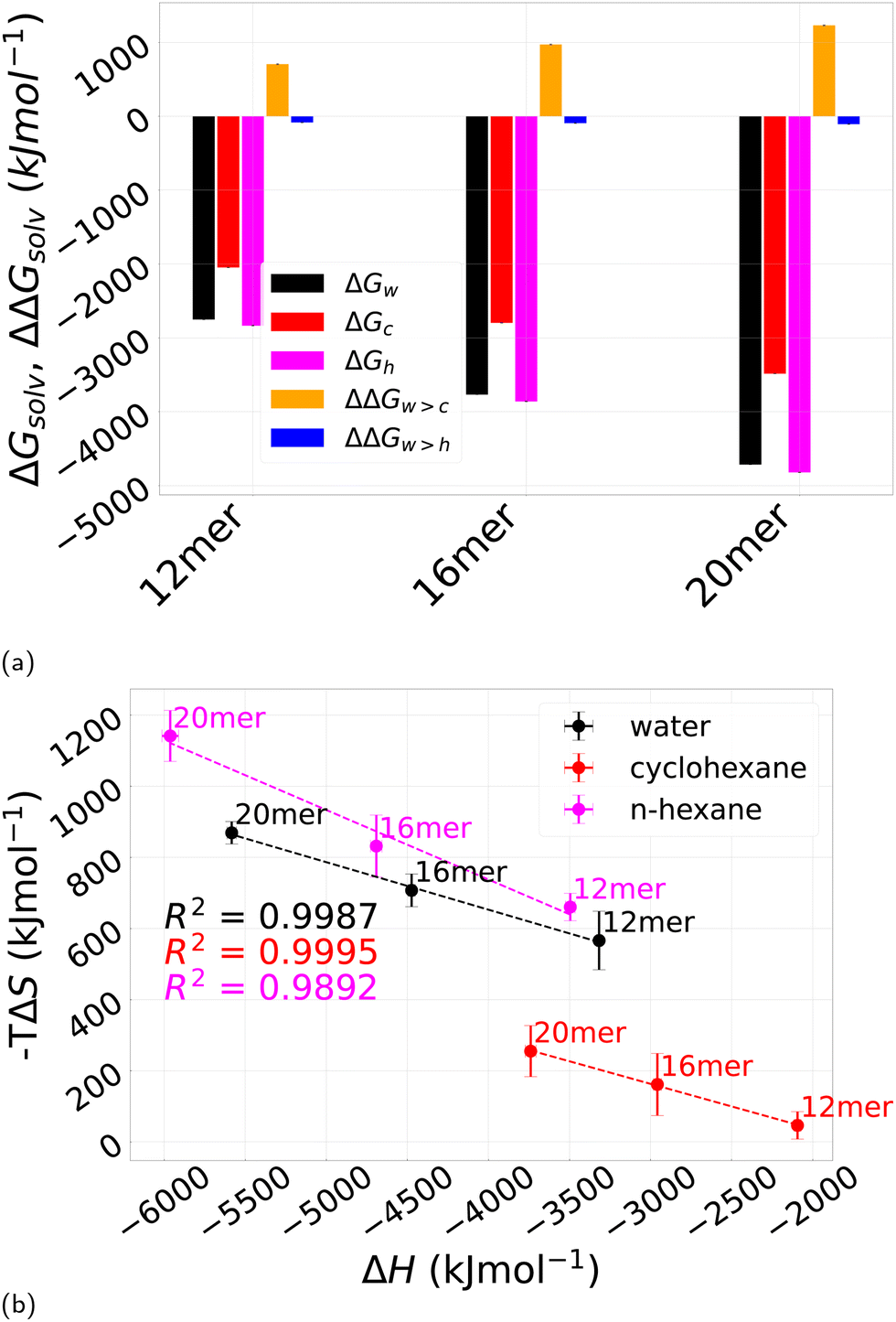Fig. 14 (a) Solvation free energy for pPA in the three different solvents studied in this work, water H₂O ΔG_w (black), cyclohexane cC₆H₁₂ ΔG_c (red), and n-hexane nC₆H₁₄ ΔG_h (magenta). Transfer free energies ΔΔG_w>c from water H₂O to cyclohexane cC₆H₁₂ (orange) and ΔΔG_w>h from water H₂O to n-hexane nC₆H₁₄ (blue) at 25 °C are also reported. Each block refers to the considered polymer length: left 12mer, middle 16mer and right 20mer; (b) entropic contribution −TΔS of ΔG_solv as a function of the enthalpic counterpart ΔH in the case of water H₂O (black) (slope −0.133), cyclohexane cC₆H₁₂ (red) (slope −0.127) and n-hexane nC₆H₁₄ (magenta) (slope −0.195).

Once more, this behavior appears to be very different when contrasted with the solvation behavior of polypeptides in the same solvents⁸ in particular with one that was not considered in previous study,⁸ and that will be discussed in the next section.

3.9 Solvation free energy of polyphelylanaline (polyPHE) oligopeptides

An important outcome of our previous findings is that hydrogen bonds do not play any role in the stabilization of the final helical structure. This is at variance with polypeptides where intra-chain hydrogen bonding is known to be a key factor in the formation of the secondary structures.⁶⁰ Then it comes as no surprise that the helix formed by pPA has a morphology very different from those formed by biopolymers.¹¹ In our previous study,⁸ the solvation process of seven polypeptides was studied in both water and cyclohexane. Similarly to the present case, the solute polarity was found to control the folding, with the solvent polarity playing a more marginal role. Unlike the present case, however, the entropic contribution in water was found to play a pivotal role.

To clarify this point, we consider here the folding process of polyphenylalanine (PHE), one of the additional polypeptides that was not included in ref. 8. One important feature of this peptide is to have a hydrophobic side chain due to its benzyl chemical structure, as illustrated in Fig. 15, whereas the backbone is significantly polar.⁸ Hence it is akin to an amphiphilic polymer⁴³ and it shares some similarities with pPA, albeit the distribution of the polar and hydrophobic moieties is very different from one another. Fig. 16a displays the solvation free energy in water H₂O ΔG_w of PHE with different number of residues from 3 to 11. In all cases it is large and negative. The same calculation in cyclohexane cC₆H₁₂ also reports a negative solvation free energy ΔG_c (Fig. 16a) even larger in magnitude. As a result the transfer free energy from water to cyclohexane ΔG_w>c is also negative (Fig. 16a) indicating that cyclohexane is a “poorer” solvent for PHE compared to water, and hence the corresponding folded state is more stable by a large margin. It is interesting to compare this result with the other hydrophobic polypeptides analyzed in ref. 8 (glycine, alanine, isoleucine) that also display negative ΔG_w>c (see Fig. 6 in ref. 8) but nearly two orders of magnitude smaller, at the same temperature. The single enthalpic and entropic contributions reported in Fig. 16b (black for water and red for cyclohexane) also display a significant difference with each other and with those of the other studied hydrophobic peptides (see Fig. 7 in ref. 8). In water (black solid line) the enthalpic gain is slightly larger that the entropic loss, thus resulting into a small solvation free energy gain reported in Fig. 16a – a value ΔG_w = 0 indicating an optimal enthalpy–entropy compensation.⁸ In cyclohexane (red line), the enthalpic gain is nearly equivalent to the solvation free energy gain and the entropic loss is significantly smaller, thus originating the large solvation free energy gain reported in Fig. 16b. A comparison with the results of other hydrophobic peptides (see Fig. 7 in ref. 8) also proves instructive. At variance with PHE, in glycine, alanine and isoleucine the slopes of the two curves are nearly identical, albeit in water the values are much smaller than in cyclohexane, similarly to what we find here for polyphenylanaline PHE.

Fig. 15 Initial stretched undeca-phenylalanine (PHE) structure.

Fig. 16 (a) Solvation ΔG_s and transfer ΔΔG_s free energy of polyphenylanaline oligopeptides of different length in water H₂O and in cyclohexane cC₆H₁₂ at 25 °C. (b) Entropic contribution −TΔS of the solvation free energy ΔG_s as a function of the enthalpic counterpart ΔH in the case of water H₂O (black) (slope −0.747) and cyclohexane cC₆H₁₂ (red) (slope −0.109). Other relevant data are reported in ESI† Fig. SXIV, SSXV, SSXVI and SSXVII and Table SV.

4 Conclusions

In this study we have addressed the relation between solvent quality, solvent polarity, and solvation free energy in the framework of the poly-polyphenylacetylene (pPA) polymer that has attracted considerable attention in the past in view of its important technological applications.^9,38,47–52 The equilibrium properties of pPA are of considerable interest because this foldamer tend to adopt a helical structure in water and other solvents and this opens up interesting perspectives associated with the helicity.⁴⁶ While this polymer can be classified as mainly hydrophobic, it forms hydrogen bond with water due to the presence of the polar moiety in its repeated unit. In order to be able to fully exploit these potential applications, however, a full control of the folding propensity is required. In this study, we specifically addressed this problem with a particular emphasis on the dependence on the solvent polarity, using the common practice of assuming the dielectric constant as a proxy for the solvent polarity.⁵ This study was carried out in several successive steps.

First, we have revisited the simple problem of a bead-spring Kramer–Grest polymer in explicit solvent,¹³ and shown that lowering the solvent quality is not equivalent to lowering the temperature, as often tacitly assumed based on implicit solvent models. This simple example allowed us to identify the correct approach required to tackle the equilibrium properties of pPA in solvents with different qualities and polarities.

Following ref. 42, we then assessed the ‘hydrophobicity’ of two paradigmatic organic solvents, cyclohexane cC₆H₁₂ and n-hexane nC₆H₁₄, in terms of their mean force potentials in water. We found that the two solvents have similar hydrophobicities although with some quantitative differences related to their different shapes.

We then performed constant temperature and pressure molecular dynamics of (pPA)_m in water H₂O (polar), in cyclohexane cC₆H₁₂, and in n-hexane nC₆H₁₄ for different number of monomers m = 12, 16, 20. Although there exist few previous experimental^9,38 and computational^50–52 studies for similar polymers and solvents, to the best of our knowledge this is the first systematic computational study of this type. We found that pPA forms stable helices in water (for sufficiently long oligomers), marginally stable in n-hexane, and unstable helices in cyclohexane.

As cyclohexane and n-hexane have similar chemical composition and hydrophobicity (Fig. 6) but different shapes, their entropy changes upon folding of the polymer might be different.⁶² The significant difference between water and the two organic solvents, and the small – but relevant, difference between cyclohexane and n-hexane, was further assessed by measuring the distribution of the bending and dihedral angles that were found to reflect the above differences. Other order parameters such as the radius of gyration R_g, the root-mean-square-deviation (RMSD) from the initial extended conformation, and the solvent accessible surface area (SASA), confirm these findings. Using two of them (R_g and RMSD) as “reaction coordinates”, we further performed a free energy landscape analysis which provided consistency to this scenario with the existence of well defined deep minimum in the case of water, two broader and shallow minima in the case of cyclohexane, and something in between for n-hexane (Fig. 11).

We further registered that the number of hydrogen bonds formed by pPA with water is essentially unchanged during the folding process, with no formation of intra-chain hydrogen bonding. Hence, hydrogen bonds do not contribute to the stability of the folded state at variance of the case of peptides.^8,51 The remaining non-covalent interactions (Lennard-Jones and Coulomb) were also monitored during the evolution. We find Lennard-Jones contribution to be negative in water, and positive in both cyclohexane and n-hexane. However, this contribution is largely overwhelmed by the Coulomb contribution that is negative for all three solvents, and significantly larger in magnitude. This suggests that the folding process is mainly enthalpically driven, with the main contribution electrostatic in nature, and largely independent of the solvent. As the chain folds driven by π–π stacking, the highly negatively charged oxygen atoms of each monomer likely combine with the positively charged hydrogen atoms of the adjacent turns, dictating the specific shape of the folded state.

Our study covers up ≈100 ns of the complete folding pathways from a linear random swollen coil, to a structured, ordered helical-like fold, in explicit solvents of different polarities, well beyond a previous computational study which could only assess the stability of the pre-organized oligomer fold, using implicit solvent and a different side chain.¹⁰

In the final step, we used thermodynamic integration to evaluate the solvation free energy of transfering a pPA single polymer from a gas phase to each of the three considered solvents. We found a negative value in all three cases, indicating a stabilizing effect of all three solvents. However, their relative stability was found to be different as assessed by the relative transfer free energies from water to cyclohexane (positive) and from water to n-hexane (negative). By monitoring the temperature dependence of these solvation free energies it was possible to separate out the enthalpic and entropic contributions. In all three solvents, we found a large dominance of the enthalpic part, but with water and n-hexane behaving similarly and differently from cyclohexane, coherently with previous results.

The same calculation carried out on phenylalanile (PHE) oligopeptides underscores the significant differences with pPA. In this case, the PHE peptide shows the expected “entropy–enthalpy compensation” in water, with a nearly perfect anticorrelation dependence (slope ≈ −1) in the −TΔS–ΔH plane. By contrast, in cyclohexane the peptide behaves similarly to pPA.

The apparent insensitivity of the entropy/enthalpy ratio for pPA in all three solvents is quite puzzling, especially when compared with the response of oligopeptides such as the PHE analyzed here. It could be very well possible that pPA has a different response at temperatures outside the range considered in the present study (270–330 K) that is the typical range of interest for oligopeptides but not necessarily for synthetic polymers. These considerations certainly warrant future studies along these lines.

While not fully conclusive, our findings recapitulate and rationalize some open issues in past results on this class of synthetic foldamers. There exist other systems where similar features might be envisaged. For instance, it is known that the degree of association in Grignard compounds is strongly dependent on the details of the solvent.^63,64 We hope that our findings will trigger further efforts in all these systems that are far from being fully understood.

All the reported simulation findings are from single-molecule runs. Motivated by present results, it would be very interesting to study the self-assembly properties of many pPA oligomers in the three different solvents considered in the present study. This is indeed part of the on-going effort by our group on the self-assembly of many chain polymer in solution, part of which has been already reported elsewhere.^65–67 We hope to be able to provide further insights on this system too in the near future.

Author contributions

CJDF: software, formal analysis, methodology, visualization, original draft preparation, review & editing. TA: software, formal analysis, visualization. TS: software, formal analysis, visualization, review & editing. AG: conceptualization, formal analysis, methodology, funding acquisition, original draft preparation, supervision, review & editing.

Data availability

The data supporting this article have been included as part of the ESI.†

Conflicts of interest

There are no conflicts to declare.

Acknowledgements

The uses of the SCSCF and vHPC multiprocessor clusters at the Università Ca’ Foscari Venezia are gratefully acknowledged. We acknowledge the CINECA awards HP10CGFUDT, HP10C1XOOJ, HP10CEB73V, HP10C7XMSY and HP10CG92F4 for the availability of high-performance computing resources and support under the ISCRA initiative. The work was supported by MIUR PRIN-COFIN2022 grant 2022JWAF7Y (AG). The authors would like to acknowledge networking support by the COST Action CA17139. Enlightening discussions with Jayanth Banavar, Michele Cascella, Amos Maritan, Davide Marcato, George Rose, and Angelo Rosa are also gratefully acknowledged.

Notes and references

1. M. Doi and S. F. Edwards, The Theory of Polymer Dynamics (International Series of Monographs on Physics), Clarendon Press, 1988.
2. P.-G. De Gennes, Scaling concepts in polymer physics, Cornell University Press, 1979.
3. A. R. Khokhlov, A. Y. Grosberg and V. S. Pande, Statistical Physics of Macromolecules (Polymers and Complex Materials), American Institute of Physics, 1994th edn, 2002.
4. M. Rubinstein and R. H. Colby, Polymer Physics (Chemistry), Oxford University Press, 1st edn, 2003.
5. T. R. Griffiths and D. C. Pugh, Coord. Chem. Rev., 1979, 29, 129–211.
6. A. R. Leach, Molecular modelling: principles and applications, Pearson Education, 2001.
7. A. Y. Ben-Naim, Hydrophobic interactions, Springer Science & Business Media, 2012.
8. C. J. Dongmo Foumthuim and A. Giacometti, Phys. Chem. Chem. Phys., 2023, 25, 4839–4853.
9. J. C. Nelson, J. G. Saven, J. S. Moore and P. G. Wolynes, Science, 1997, 277, 1793–1796.
10. S. Sen, J. Phys. Chem. B, 2002, 106, 11343–11350.
11. J. R. Banavar, A. Giacometti, T. X. Hoang, A. Maritan and T. Škrbić, Proteins: Struct., Funct., Bioinf., 2023 DOI:10.1002/prot.26567.
12. K. Kremer and G. S. Grest, J. Chem. Phys., 1990, 92, 5057–5086.
13. Y. Huang and S. Cheng, J. Polym. Sci., 2021, 59, 2819–2831.
14. J. D. Weeks, D. Chandler and H. C. Andersen, J. Chem. Phys., 1971, 54, 5237–5247.
15. S. Plimpton, J. Comput. Phys., 1995, 117, 1–19.
16. A. P. Thompson, H. M. Aktulga, R. Berger, D. S. Bolintineanu, W. M. Brown, P. S. Crozier, P. J. in’t Veld, A. Kohlmeyer, S. G. Moore, T. D. Nguyen, R. Shan, M. J. Stevens, J. Tranchida, C. Trott and S. J. Plimpton, Comput. Phys. Commun., 2022, 271, 108171.
17. L. Verlet, Phys. Rev., 1967, 159, 98.
18. W. Shinoda, M. Shiga and M. Mikami, Phys. Rev. B: Condens. Matter Mater. Phys., 2004, 69, 134103.
19. N. M. O’Boyle, M. Banck, C. A. James, C. Morley, T. Vandermeersch and G. R. Hutchison, J. Cheminf., 2011, 3, 33.
20. J. Wang, R. M. Wolf, J. W. Caldwell, P. A. Kollman and D. A. Case, J. Comput. Chem., 2004, 25, 1157–1174.
21. J. Wang, W. Wang, P. A. Kollman and D. A. Case, J. Mol. Graphics Modell., 2006, 25, 247–260.
22. K. Lindorff-Larsen, S. Piana, K. Palmo, P. Maragakis, J. L. Klepeis, R. O. Dror and D. E. Shaw, Proteins: Struct., Funct., Bioinf., 2010, 78, 1950–1958.
23. A. W. Sousa da Silva and W. F. Vranken, BMC Res. Notes, 2012, 5, 1–8.
24. A. Jakalian, B. L. Bush, D. B. Jack and C. I. Bayly, J. Comput. Chem., 2000, 21, 132–146.
25. A. Jakalian, D. B. Jack and C. I. Bayly, J. Comput. Chem., 2002, 23, 1623–1641.
26. W. L. Jorgensen, J. Chandrasekhar, J. D. Madura, R. W. Impey and M. L. Klein, J. Chem. Phys., 1983, 79, 926–935.
27. C. J. Dongmo Foumthuim, M. Carrer, M. Houvet, T. Škrbić, G. Graziano and A. Giacometti, Phys. Chem. Chem. Phys., 2020, 22, 25848–25858.
28. G. Bussi, D. Donadio and M. Parrinello, J. Chem. Phys., 2007, 126, 014101.
29. B. Hess, H. Bekker, H. J. C. Berendsen and J. G. E. M. Fraaije, J. Comput. Chem., 1997, 18, 1463–1472.
30. M. Parrinello and A. Rahman, J. Appl. Phys., 1981, 52, 7182–7190.
31. R. Sarma and S. Paul, J. Chem. Phys., 2011, 135, 174501.
32. R. Sarma and S. Paul, J. Phys. Chem. B, 2012, 116, 2831–2841.
33. Y. M. Muñoz-Muñoz, G. Guevara-Carrion, M. Llano-Restrepo and J. Vrabec, Fluid Phase Equilib., 2015, 404, 150–160.
34. W. L. Jorgensen, J. D. Madura and C. J. Swenson, J. Am. Chem. Soc., 1984, 106, 6638–6646.
35. R. Fantoni, A. Giacometti and A. Santos, J. Chem. Phys., 2015, 142, 224905-1–224905-17.
36. H. Garg, R. Rajesh and S. Vemparala, J. Chem. Phys., 2023, 158, 114903-1–114903-10.
37. P. Gallo, K. Amann-Winkel, C. A. Angell, M. A. Anisimov, F. Caupin, C. Chakravarty, E. Lascaris, T. Loerting, A. Z. Panagiotopoulos and J. Russo, et al. , Chem. Rev., 2016, 116, 7463–7500.
38. R. B. Prince, J. G. Saven, P. G. Wolynes and J. S. Moore, J. Am. Chem. Soc., 1999, 121, 3114–3121.
39. Y. D. Fomin, V. N. Ryzhov and E. N. Tsiok, J. Chem. Phys., 2015, 143, 184702.
40. R. Boese, H.-C. Weiss and D. Bläser, Angew. Chem., Int. Ed., 1999, 38, 988–992.
41. G. Herzberg, Electronic spectra and electronic structure of polyatomic molecules, Van Nostrand, 1966.
42. D. E. Smith and A. D. J. Haymet, J. Chem. Phys., 1993, 98, 6445–6454.
43. V. V. Vasilevskaya, P. G. Khalatur and A. R. Khokhlov, Macromolecules, 2003, 36, 10103–10111.
44. D. J. Hill, M. J. Mio, R. B. Prince, T. S. Hughes and J. S. Moore, Chem. Rev., 2001, 101, 3893–4012.
45. B. Teng, J. Atcher, L. Allmendinger, C. Douat, Y. Ferrand and I. Huc, Org. Biomol. Chem., 2023, 21, 3525–3530.
46. F. Freire, E. Quinoa and R. Riguera, Chem. Rev., 2016, 116, 1242–1271.
47. M. S. Gin, T. Yokozawa, R. B. Prince and J. S. Moore, J. Am. Chem. Soc., 1999, 121, 2643–2644.
48. R. B. Prince, S. A. Barnes and J. S. Moore, J. Am. Chem. Soc., 2000, 122, 2758–2762.
49. W. Y. Yang, R. B. Prince, J. Sabelko, J. S. Moore and M. Gruebele, J. Am. Chem. Soc., 2000, 122, 3248–3249.
50. S. Elmer and V. S. Pande, J. Phys. Chem. B, 2001, 105, 482–485.
51. S. Sen, J. Phys. Chem. B, 2002, 106, 11343–11350.
52. S. P. Elmer and V. S. Pande, J. Chem. Phys., 2004, 121, 12760–12771.
53. T. Qi, V. Maurizot, H. Noguchi, T. Charoenraks, B. Kauffmann, M. Takafuji, H. Ihara and I. Huc, Chem. Commun., 2012, 48, 6337–6339.
54. B. Chu, Q. Ying and A. Y. Grosberg, Macromolecules, 1995, 28, 180–189.
55. T. Škrbić, A. Maritan, A. Giacometti, G. D. Rose and J. R. Banavar, Phys. Rev. E, 2021, 104, 014402.
56. A. Spanò, L. Fanton, D. C. Pizzolato, J. Moi, F. Vinci, A. Pesce, C. J. Dongmo Foumthuim, A. Giacometti and M. Simeoni, BMC Bioinf., 2023, 24, 336.
57. S. Wijesinghe, S. Maskey, D. Perahia and G. S. Grest, J. Polym. Sci., Part B: Polym. Phys., 2016, 54, 582–588.
58. F. Eisenhaber, P. Lijnzaad, P. Argos, C. Sander and M. Scharf, J. Comput. Chem., 1995, 16, 273–284.
59. L. Dal Compare, F. Romano, J. A. Wood, A. Widmer-Cooper and A. Giacometti, J. Chem. Phys., 2023, 159, 174905.
60. L. Pauling, R. B. Corey and H. R. Branson, Proc. Natl. Acad. Sci. U. S. A., 1951, 37, 205–211.
61. M. Carrer, T. Skrbic, S. L. Bore, G. Milano, M. Cascella and A. Giacometti, J. Phys. Chem. B, 2020, 124, 6448–6458.
62. S. Asakura and F. Oosawa, J. Polym. Sci., 1958, 33, 183–192.
63. F. W. Walker and E. Ashby, J. Am. Chem. Soc., 1969, 91, 3845–3850.
64. M. de Giovanetti, S. H. Hopen Eliasson, A. C. Castro, O. Eisenstein and M. Cascella, J. Am. Chem. Soc., 2023, 145, 16305–16309.
65. D. Marcato, A. Giacometti, A. Maritan and A. Rosa, J. Chem. Phys., 2023, 159, 154901.
66. T. Arcangeli, T. Škrbijć, S. Azote, D. Marcato, A. Rosa, J. R. Banavar, R. Piazza, A. Maritan and A. Giacometti, Phase behaviour and self-assembly of semiflexible polymers in poor-solvent solutions, 2024, https://arxiv.org/abs/2405.11287.
67. D. Marcato, A. Giacometti, A. Maritan and A. Rosa, Assessing Polymer Phase Behavior in Explicit Solvent and with Vacancies, 2024, https://arxiv.org/abs/2407.01590.

---

Footnote

† Electronic supplementary information (ESI) available: Additional results, including figures and tables. See DOI: https://doi.org/10.1039/d4sm00727a

---