
 Open Access Article
 This Open Access Article is licensed under a
 Creative Commons Attribution 3.0 Unported Licence
Phase separation in soft repulsive polymer mixtures: foundation and implication for chromatin organization
Naoki
Iso
,
Yuki
Norizoe
and
Takahiro
Sakaue
 *
*
Department of Physical Sciences, Aoyama Gakuin University, 5-10-1 Fuchinobe, Chuo-ku, Sagamihara, Japan. E-mail: sakaue@phys.aoyama.ac.jp
First published on 19th August 2024
Abstract
Given the wide range of length scales, the analysis of polymer systems often requires coarse-graining, for which various levels of description may be possible depending on the phenomenon under consideration. Here, we provide a super-coarse grained description, where polymers are represented as a succession of mesosopic soft beads which are allowed to overlap with others. We then investigate the phase separation behaviors in a mixture of such homopolymers based on mean-field theory, and discuss universal aspects of the miscibility phase diagram in comparison with the numerical simulation. We also discuss an extension of our analysis to mixtures involving random copolymers, which might be interesting in the context of chromatin organization in a cell nucleus.
1 Introduction
Phase separation in polymer solutions and blends have a long history of research due to its importance in fundamental science as well as industrial applications.1–7 Recently, its pivotal role in the field of biophysics has been recognized as a basic mechanism to organize various cellular and nuclear bodies.8–19 Here, given the complexity of biological systems, standard approaches such as the Flory–Huggins theory to analyze the phase separation do not always suffice, and various extensions or modifications may be called for depending on the phenomena under consideration.In this paper, we provide one such example, where we investigate the phase separation behavior of polymer mixtures made of mesoscopic segments. Our work has been motivated by the recent attempts to simulate chromatin organization in a cell nucleus. In ref. 20, Fujishiro and Sasai constructed a polymer model of the whole genome of human cells, where each chromatin is modeled as a succession of soft-core monomers. Here, individual monomers (beads) represent ∼102 kbp of DNA, which is much larger than the conventional monomers defined in a standard theory or simulation of polymer systems. They argued that the interaction between such mesoscopic segments is soft and repulsive, and the imbalance in this repulsion in systems with e.g., eu- and hetero-chromatic monomers would trigger the phase separation. Similar modeling of the large scale behavior of chromatin with a soft-core potential naturally arises after the coarse-graining, hence has been employed in other studies as well,21–25 where the soft potential incorporates the entropic effect relevant to the mesoscopic segments.
How can we describe such phase separation phenomena in chromatin theoretically? The immediate complication lies in the copolymer nature of the chromatin model.21,26 However, even if we leave aside the sequence effect and restrict our attention to a binary mixture of homopolymers, the application of the Flory–Huggins theory is hampered because of the allowed overlap between monomers due to the soft-core nature of the inter-monomer potentials. A key insight would thus be obtained by the phase behavior of the mixture of soft particles. This problem has been extensively studied by groups of Likos, Löwen and Kahl.27–29 Very recently, Sta![[n with combining breve]](https://www.rsc.org/images/entities/char_006e_0306.gif) o, Likos and Egorov have extended the framework to a system of chains of soft beads.30 Although their primary target is a mixture of linear polymers and ring polymers (or polycatenanes), we expect that the same physics applies to the chromatin system, too.
o, Likos and Egorov have extended the framework to a system of chains of soft beads.30 Although their primary target is a mixture of linear polymers and ring polymers (or polycatenanes), we expect that the same physics applies to the chromatin system, too.
Our first aim is thus to recapitulate and to numerically validate the theoretical framework for the binary mixture of polymers made of soft monomers, which allows one to analyze the phase behavior. In Section 2, we introduce the mean-field free energy for our system. From the analysis of the free energy, we present in Section 3 the miscibility phase diagram and compare it with the result from molecular dynamics (MD) simulations. Section 4 is devoted to discussions on universal aspects of the phase diagram, comparison with a conventional Flory–Huggins theory, and connection to the Gaussian core model. Building on the framework, we also discuss its extension to a system containing copolymers in Section 5.
2 Free energy of the soft repulsive polymer mixture
Following Stao,30 we adopt the following free energy density for the mixture of polymers modeled as the succession of soft beads which represent mesoscopic segments | (1) |
Note that in this representation, the parameters χxy have a unit of volume, and we measure them in units of the volume of individual beads. In other words, we assume, for simplicity, the characteristic size (σ) of beads a and b are equal, which is taken to be the unit of length. Although there is no attraction, the phase separation may be induced by the asymmetry in the repulsion, i.e., χaa ≠ χbb. At first sight, eqn (1) looks like a free energy in the second virial approximation valid for low concentrations. As we will show below, however, the free energy eqn (1) is capable of describing the phase separation in the concentrated regime (ca + cb)σ3 > 1 (see Section. 4.3 for discussion).
Let us first clarify a mathematical aspect relevant to the phase equilibria condition in the system described by the free energy eqn (1). If a homogeneous mixture of polymer A and polymer B separates into phase 1 and phase 2, the demixed state is specified by the concentrations of both components in respective phases, i.e., (c(1)a, c(1)b) and (c(2)a, c(2)b). The number of unknowns is thus nu = 4. On the other hand, the phase equilibria between two phases indicates the equalities of chemical potentials μ(α)x = ∂f/∂c(α)x between two phases (α = 1 or 2) for both components (x = a or b), i.e., μ(1)a = μ(2)a and μ(1)b = μ(2)b and also the mechanical balance ensured by the equality of pressure P(1) = P(2), where P(ca, cb) = ca[∂f(ca, cb)/∂ca] + cb[∂f(ca, cb)/∂cb] − f(ca, cb), leading to the number of conditions to determine the phase equilibria nc = 3. Comparing the number of unknowns and conditions, we expect that the dimensionality of the phase boundary, i.e., binodal is dpb = nu − nc = 1.
3 Phase diagram of the soft repulsive polymer mixture
In Fig. 1(a), we show an example of the miscibility phase diagram obtained from the free energy eqn (1) under the fixed interaction parameters. As we have discussed, the phase diagram is two-dimensional spanned by ca and cb, in which the uniform state (bottom left) and the demixed state (upper right) are separated by a one-dimensional phase boundary. Tie lines, which connect (c(1)a, c(1)b) and (c(2)a, c(2)b) in the demixed state, are negatively sloped, indicating the phase separation is a segregative type. As expected, the region for demixing widens with the increase in either chain length or the repulsion strength, see Fig. 1(b). Note that despite the symmetry in the chain length Na = Nb in the examples shown here, the phase diagram exhibits asymmetry about the diagonal ca = cb. The asymmetry is caused by the difference in physical properties of type a and b beads, which leads to the phase rich in softer beads b being more concentrated than the other. This feature can be made more evident by re-plotting the phase diagram with the total concentration c = ca + cb and the composition ψ = ca/c plane (Fig. 1(c)). | ||
| Fig. 1 Miscibility phase diagram obtained from the free energy eqn (1). (a) Binodal (solid curve) and spinodal (dashed curve) in the case of repulsion parameters χaa = 2, χbb = 1, χab = 1.5 and the chain length Na = Nb = 20. Two curves meet at the critical point marked by a circle. Some examples of tie lines are also shown. (b) Dependence of the phase diagram on chain length and repulsion parameters, where binodals obtained from a different set of parameters are shown. (c) Replot of the phase diagram (a) in the plane spanned by total concentration c = ca + cb and the composition ψ = ca/c. | ||
To check the validity of the free energy prediction, we have performed numerical simulations of the polymer mixture. Briefly, the system is a mixture of two types of linear homopolymers A and B, where the A(B) polymer is made of a succession of Na(Nb) beads of type a(b) (see the appendix for details of the simulation model). To represent the soft repulsion between monomers, we employ the Gaussian potential, see eqn (15) in the appendix, where the strength of the repulsion between the x-bead and y-bead is εxy in units of kBT.
The numerically determined phase boundary shown in Fig. 2(a) is obtained with the interaction strength εaa = 2, εbb = 1, εab = 1.5 and the chain length Na = Nb = 20, where the overall concentrations are varied from (c(o)a, c(o)b) = (0.1, 0.1) to (c(o)a, c(o)b) = (0.5, 0.5). We find that the mixture is homogeneous at (c(o)a, c(o)b) = (0.1, 0.1), but develops large concentration fluctuation at (c(o)a, c(o)b) = (0.25, 0.25), and a further increase in concentration leads to a well-defined phase separated structure (Fig. 2(b)). Remarkably, the numerically determined phase diagram resembles that predicted by the free energy analysis (Fig. 1). More specifically, we find that the numerical and analytical phase diagrams almost overlap under the correspondence χxy/εxy ≃ 2.5 between the interaction parameters in free energy and the interaction strengths in simulation.
 | ||
| Fig. 2 Phase boundary (solid down-pointing triangles) of the miscibility phase diagram obtained from numerical simulation with interaction parameters εaa = 2, εbb = 1, εab = 1.5 and the chain length Na = Nb = 20. Open symbols (square, circle and triangle) indicate the overall concentrations of the system simulated; a square or triangle indicates that the uniform state is stable or unstable, while a circle represents the vicinity of the critical point. (a) The overlapped solid curve is the binodal curve obtained from mean field theory with χaa = 5, χbb = 2.5, χab = 3.75. (b) Spatial profile of concentration of the a-bead under various overall concentrations. (c) Histogram of the number density of the a-bead, where the horizontal axis represents the deviation from the uniform concentration ca − c(o)a. | ||
4 Discussions
4.1 General aspects of the phase diagram
In Section 3, we have shown one example of how the phase boundary alters with the change in chain length or the interaction strength (Fig. 1(b)). To clarify the dependence of the shape of the phase diagram on the system parameters in a more systematic way, it is desirable to determine the universal aspects inherent to the model described by the free energy eqn (1).To this end, we introduce the rescaled concentrations ![[c with combining tilde]](https://www.rsc.org/images/entities/i_char_0063_0303.gif) a = caNaχaa and b = cbNbχbb, which enables us to rewrite eqn (1) as
a = caNaχaa and b = cbNbχbb, which enables us to rewrite eqn (1) as
 | (2) |
 | (3) |
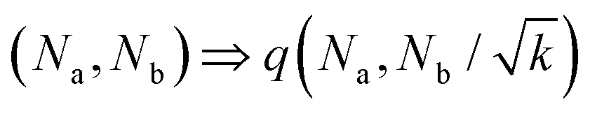
 constant. These conditions are satisfied by the following transformations
 | (4) |
 | (5) |
o et al.30 Indeed, from the stability analysis of the uniform state, one finds the spinodal curve | (6) |
 | (7) |
 , and eqn (7) determines the location of the critical point on the spinodal curve.30 In Fig. 3, we demonstrate a collapse of the phase diagram upon rescaling.
 | ||
Fig. 3 Rescaling of phase diagram. Phase boundaries for three different conditions with common families specified by (a) k1 = 2,  and (b) k1 = 1.4, and (b) k1 = 1.4,  . In (a), the parameters of one of the three conditions shown here are set to (χaa, χbb, χab, Na, Nb) = (2, 1, 1.5, 20, 20) and the other two are obtained from the transformations eqn (4) and (5) with p = 0.25, q = 1, k = 4 (blue) and p = 2, q = 0.5, k = 0.25 (green). In (b), the reference parameters are set to (χaa, χbb, χab, Na, Nb) = (4.2, 3, 3.6, 20, 20) and the other two are obtained from the transformations eqn (4) and (5) with p = 1, q = 0.5, k = 4 (blue) and p = 0.25, q = 2, k = 1 (green). (c) and (d) are master curves of the phase diagrams for the family with k1 = 2, . In (a), the parameters of one of the three conditions shown here are set to (χaa, χbb, χab, Na, Nb) = (2, 1, 1.5, 20, 20) and the other two are obtained from the transformations eqn (4) and (5) with p = 0.25, q = 1, k = 4 (blue) and p = 2, q = 0.5, k = 0.25 (green). In (b), the reference parameters are set to (χaa, χbb, χab, Na, Nb) = (4.2, 3, 3.6, 20, 20) and the other two are obtained from the transformations eqn (4) and (5) with p = 1, q = 0.5, k = 4 (blue) and p = 0.25, q = 2, k = 1 (green). (c) and (d) are master curves of the phase diagrams for the family with k1 = 2,  and k1 = 1.4, and k1 = 1.4,  , respectively, upon rescaling of original phase diagrams (a) and (b). , respectively, upon rescaling of original phase diagrams (a) and (b). | ||
4.2 Comparison with Flory–Huggins theory
It is instructive to compare the present theory with the standard Flory–Huggins theory for polymer blends. The Flory–Huggins free energy (per lattice site) for a blend of polymer A and B is written as12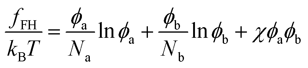 | (8) |
Fig. 4 shows the phase diagram calculated from eqn (8). When we fix the interaction parameter at the value χ > χc, where  is the critical value for the phase separation, the phase diagram as a function of ϕa is a one-dimensional line with two points ϕ(1)a and ϕ(2)a representing the phase boundaries. If the overall concentration falls in between these two points, the uniform state is metastable (outside the spinodal region) or unstable (inside the spinodal region) and the system phase separates into the A-poor (dilute) and A-rich (concentrated) phases with the volume fractions ϕ(1)a and ϕ(2)a, respectively. Note that the dimensionality of the phase boundary at fixed χ is dpb = 0, i.e., points, which is a consequence of the equality of the number of conditions (nc = 2, i.e., μ(1)a = μ(2)a and μ(1)b = μ(2)b) and the number of unknowns (nu = 2, i.e., ϕ(1)a and ϕ(2)a). We note that a set of conditions μ(1)a = μ(2)a and μ(1)b = μ(2)b is equivalent to μ(1)a = μ(2)a and Π(1) = Π(2), where Π(ϕa) = ϕa[dfFH(ϕa)/dϕa] − fFH(ϕa) is the osmotic pressure, the use of which may be more common in polymer solution, where component b is regarded to be a solvent. These two methods are equivalent due to the relationship
| −Π(ϕa)v0 = μb(ϕa), | (9) |
 | ||
| Fig. 4 (a) Miscibility phase diagram for a polymer blend obtained from Flory–Huggins free energy eqn (8). (b) Under a fixed χ-parameter (χ > χc), the phase boundaries are points (dpb = 0) on a line. | ||
It is also known that the interaction part in the Flory–Huggins free energy initially takes the form (χaa/2)ϕa2 + (χbb/2)ϕb2 + χabϕaϕb. Rewriting it into the form of eqn (8) with a single parameter χ = χaa/2 + χbb/2 − χab is done using the incompressibility condition. Again, it does not apply to our soft polymer description. Since our system originally possesses three components, we naturally need three interaction parameters to characterize the system. We also note that the critical χ parameter in blends of long polymers Na, Nb ≫ 1 is χc → 0 in Flory–Huggins theory. A necessary condition for the phase separation in this limit is thus χ > 0 ⇔ (χaa + χbb)/2 > χab. In contrast, as discussed in Section 4, the corresponding condition in our soft polymer mixtures is 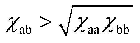 independent of the chain length.30
4.3 Relationship with the Gaussian core model
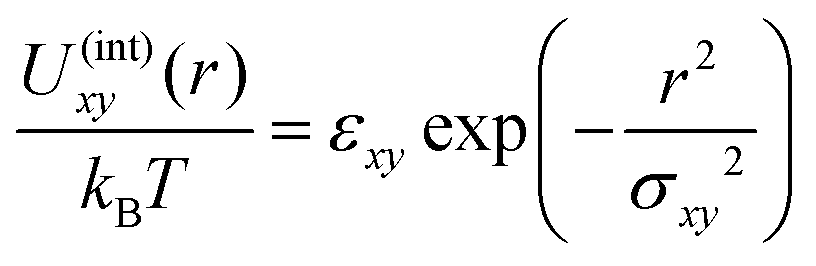
In our model, polymers are described as N successive soft beads, where these beads are already mesoscopic entities with their internal degrees of freedom integrated out. We note here that, starting from a microscopic model, there is a freedom to choose N, i.e., the degree of the coarse-graining. Although the extreme limit of the choice is N = 1, in which individual polymers are described as single soft particles, the validity of such a description may break down at high concentration.31It is known that the effective pair potential between two isolated polymer coils in dilute solution can be well approximated using a simple Gaussian potential
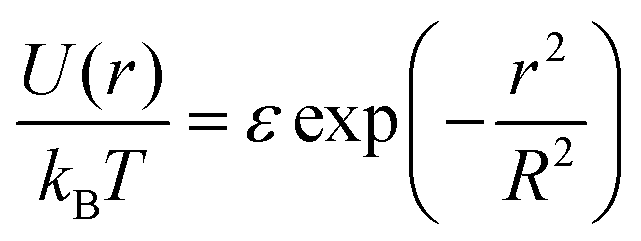 | (10) |
Another point deserving comment is the relationship between the strength of the interaction potential εxy and the interaction parameter χxy in our free energy eqn (1). We have shown in Section 3 that the simulation results quantitatively match with the free energy prediction under the relationship χxy/εxy ≃ 2.5. Since the free energy (1) takes apparently the same form as the virial expansion up to the second order, one may expect that the εxy − χxy relationship would be obtained from  . As emphasized in ref. 32 however, the free energy eqn (1) is based on the random phase approximation (RPA).33 As such, it becomes more and more accurate in higher concentration regimes in contrast to the second virial approximation.33 In fact, unlike the virial expansion, the quadratic form of the free energy in concentrations is a consequence of the RPA closure, where the direct correlation functions, which appear in the Ornstein–Zernike relationship, is independent of the concentrations. The analysis of the equation of state with RPA leads to the identification
  . Given the resultant ratio χxy/εxy = π3/2 is considered to be an upper bound compared to a more accurate estimate e.g., obtained from hypernetted chain closure,32 we find our result χxy/εxy ≃ 2.5 reasonable and providing an overall consistency of the soft core model description of the phase separation based on the free energy eqn (1).
5 Mixtures with random copolymers
So far we have discussed a foundation for the coarse-grained description of a polymer mixture, where polymers are represented as a succession of soft mesoscopic beads. In particular, we have focused on the phase behavior of a mixture of homopolymers. As stated in the introduction, however, one of the main motivations to necessitate such a description is its relevance to describe the large scale behavior of chromatin in a cell nucleus. In this section, we would like to discuss a simple extension of our theory, which may be linked to a certain aspect of chromatin organization in living cells.It is known that interphase chromatin in early embryos is quite homogeneous inside the nucleus, which is, in a certain sense, reminiscent to a uniform solution of homopolymers.34 With the progress of the development stage, however, several characteristic structures, such as heterochromatin foci and transcriptional factories, start to appear.35 Responsible for such structure formations would be a phase separation, which is driven by local alternation of chromatin monomers caused by e.g., post-translational modification. The change in the chemical state in chromatin monomers likely induces the modulation of physical properties along the chromatin polymer, which could be represented by a copolymer model. Since the variation in repulsive forces primarily reflects the difference in the density of core-bearing monomers within the coarse-grained segments,20,36 segment “a” represents regions where chromatin exists in a relaxed, less condensed state, reminiscent of euchromatin, while segment “b” corresponds to more condensed regions akin to heterochromatin. The structure formation under consideration could thus be treated by the appearance of copolymers in the matrix of homopolymers. With this in mind, let us consider a mixture of homopolymers H (with length Nh), which is composed of type a beads only, and copolymer C (with length Nc), which is composed of type a and b beads. The monomer concentration of H and C polymers are ch and cc, respectively. For the analytical tractability in a simple mean-field description, we assume the latter to be a random copolymer, which is characterized by the fraction α of b beads, i.e., the number of b beads in a copolymer C is αNc.
The free energy of the mixture is written as
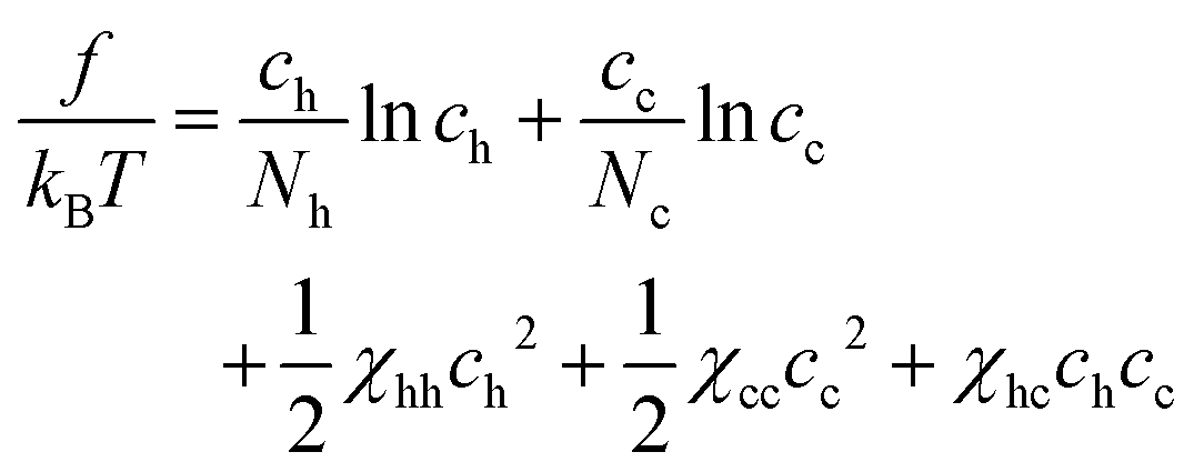 | (11) |
| χcc = (1 − α)2χaa + α2χbb + 2α(1 − α)χab | (12) |
| χhc = (1 − α)χaa + αχab | (13) |
In Fig. 5, we show phase diagrams obtained from the free energy eqn (11) with eqn (12) and (13) for a fixed α. Note that α = 0 reduces to a homopolymer solution (with only type a bead), and α = 1 corresponds to a blend of homopolymers A and B analyzed in earlier sections. Here we show the cases for α = 0.3, 0.5. As expected, the region for phase separation enlarges with the fraction α. In addition, the results depend on a relative stiffness between beads a and b. As shown, the system is more prone to phase separation when the matrix polymer is softer χaa < χbb reflecting the asymmetry in the phase diagram of homopolymer mixtures (Section 3).
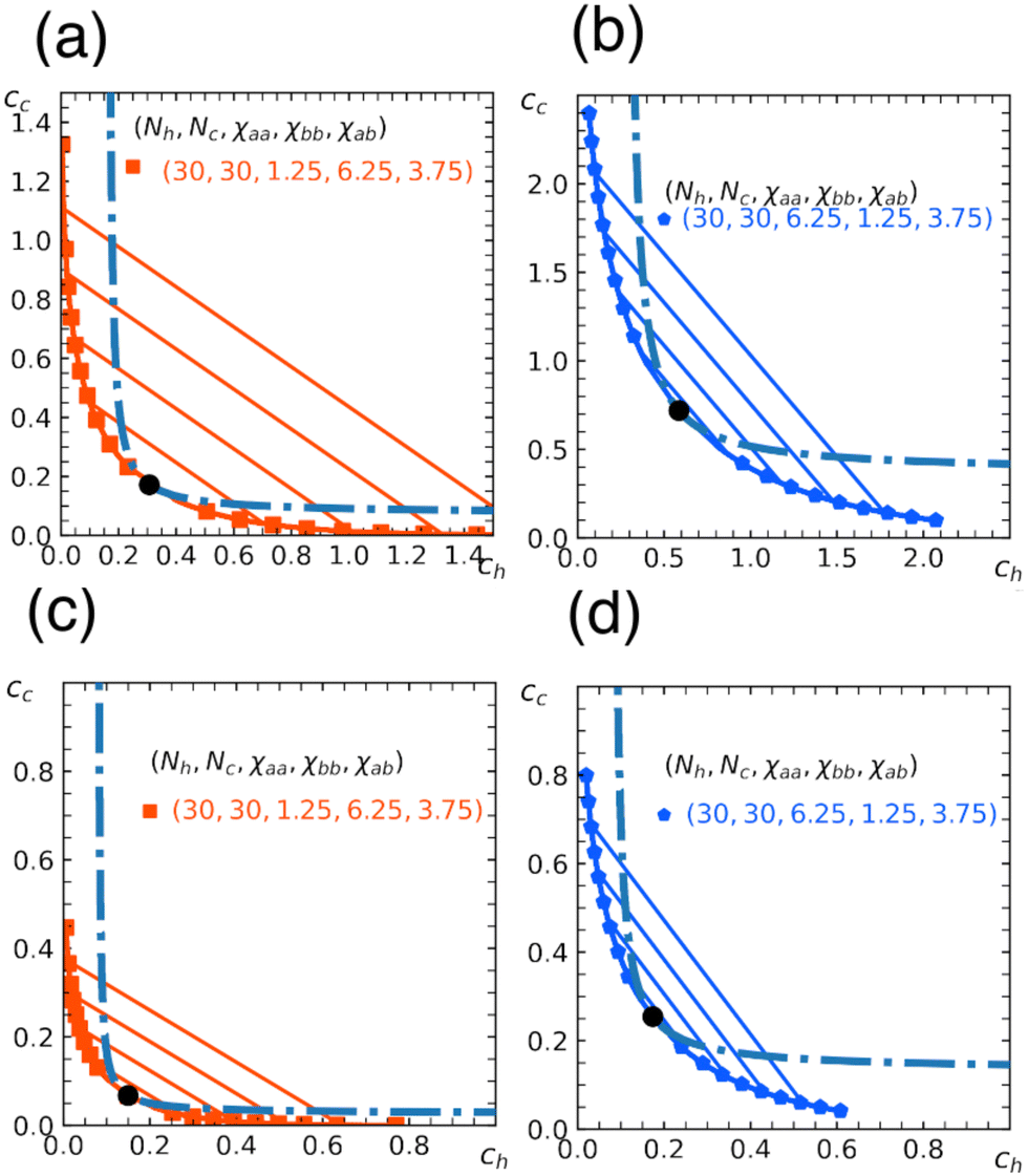 | ||
| Fig. 5 Miscibility phase diagram of homo- and copolymer mixtures obtained from the free energy eqn (11). Binodal (solid curve) and spinodal (dashed curve) for the chain length Nh = Nc = 30. Fraction of b beads in the copolymer is α = 0.3 in (a) and (b), and α = 0.5 in (c) and (d). The repulsion parameters between beads are χaa = 1.25, χbb = 6.25, χab = 3.75 in (a) and (c), and χaa = 6.25, χbb = 1.25, χab = 3.75 in (b) and (d). Critical point (marked by a circle), and some examples of tie lines are also shown. | ||
To check the validity of the free energy prediction, we again performed numerical simulations using Gaussian potentials to represent bead–bead soft repulsions. In Fig. 6 and 7, we compare the theoretical phase diagram in Fig. 5 with simulation results, where the repulsion strengths for the Gaussian potentials are set to be εxy = χxy/2.5 between beads x and y as determined from the result of the homopolymer mixtures. As shown, the agreement is rather satisfactory, demonstrating that the overall trend of phase separation is well captured by the proposed free energy. In Fig. 6 and 7, we also show the spatial profiles of the monomer concentration ch of the homopolymer together with the corresponding typical snapshots.
 | ||
| Fig. 6 Quantitative comparison of a theoretical phase diagram against the numerical simulation. Chain lengths are Nh = Nc = 30, the fraction of b beads in the copolymer is α = 0.3, and the repulsion parameters between beads are (a) χaa = 1.25, χbb = 6.25, χab = 3.75 and (b) χaa = 6.25, χbb = 1.25, χab = 3.75. These conditions correspond to those in Fig. 5(a) and (b), respectively. (Top) Binodal (solid curve) with the critical point marked by a solid circle. Open symbols indicate the overall concentration (c(0)h, c(0)c) adopted in numerical simulations performed under the parameter correspondence εxy = χxy/2.5, where open squares and triangles, respectively, indicate the one-phase and two-phase regions. In the latter, the concentrations after phase separation are shown by solid triangles, which are connected by tie lines. (Middle) Spatial profiles of the monomer concentration of H-polymer. (Bottom) Typical snapshots obtained in simulations with (c(0)h, c0)c) = (0.4, 0.4), where red beads represent type-a beads contained in the H-polymer, while yellow or blue beads represent type-a or type-b beads contained in the C-polymer, respectively. The snapshots were rendered using OVITO.37 | ||
 | ||
| Fig. 7 Quantitative comparison of the theoretical phase diagrams against the numerical simulation. Parameters are the same as those in Fig. 6 (Nh = Nc = 30, and repulsion parameters χaa = 1.25, χbb = 6.25, χab = 3.75 in (a) or χaa = 6.25, χbb = 1.25, χab = 3.75 in (b)) except for the fraction of b beads in the copolymer, which is α = 0.5 here. These conditions correspond to those in Fig. 5(c) and (d), respectively. (Top) Binodal (solid curve) with the critical point marked by the solid circle. Open symbols indicate the overall concentration (c(0)h, c(0)c) adopted in numerical simulations performed under the parameter correspondence εxy = χxy/2.5, where open squares and triangles, respectively, indicate the one-phase and two-phase regions. In the latter, concentrations after phase separation are shown by solid triangles, which are connected by tie lines. (Middle) Spatial profile of the monomer concentration of the H-polymer. (Bottom) Typical snapshots obtained in simulations with (c(0)h, c(0)c) = (0.2, 0.2), where red beads represent type-a beads contained in the H-polymer, while yellow or blue beads represent type-a or type-b beads contained in the C-polymer, respectively. The snapshots were rendered using OVITO.37 | ||
6 Discussions and summary
Numerical simulations of large scale chromatin organization in the cell nucleus often adopt highly coarse-grained models, in which the chromatin polymer is represented as a succession of soft beads.20–25 Unlike a model which employs nucleosomes as monomers of the chromatin polymer, each bead here represents a substantial amount of nucleosomes, thus regarded as a mesoscopic entity, allowing mutual overlaps with entropic penalty. It has been shown that the effective interaction between such mesoscopic segments is soft and repulsive, a qualitative feature of which is well approximated by the Gaussian potential.20We have considered binary mixtures of such soft repulsive polymers and investigated how the imbalance in repulsive interactions between different species leads to the phase separation. After summarizing universal aspects of the phase diagram based on invariant properties of the free energy upon changes in parameter values, we have extended the theory to mixtures including random copolymers, which may have some implications on chromatin phase separation.
As discussed in Section 5, the random copolymer model is inspired by epigenetic modification of chromatin. This modification is performed and maintained by enzymes, thus includes an energy consuming nonequilibrium process. In this sense, our description based on an equilibrium framework should be considered a useful effective description to elucidate the impact of phase separation on chromatin organization. The same remark applies to many current biophysical models of chromatin, not only for its structural organization but also for its dynamics. Yet, there are several other works, which emphasize possible impacts of various nonequilibrium effects on chromatin.18,38–45 Perhaps, some of these effects associated with nonequilibrium activities could be described by effective equilibrium models. This kind of strategy may well work to understand some aspect of the problem, but may fail to capture other aspects. In our opinion, it remains to be seen how and when nonequilibrium factors are critically important in chromatin biophysics. The same comment would apply to topological constraints, another factor presumably important in chromatin, but not explicitly included in our description.46,47 In this regard, it is interesting to note that as discussed in ref. 42, similar physics as described in the present paper may be important in a blend of non-concatenated ring polymers, where the soft repulsion arises from the so-called topological volume due to topological constraints.48–50
As possible extensions of our work, we first note that our theory deals with macro-phase separation, hence does not capture the possible appearance of mesophases. However, the occurrence of “micro-phase separation” is naturally expected in copolymer systems, the elucidation of which should provide further insight into the problem of chromatin organization in nuclei. Secondly, although we have only analyzed bulk properties based on mean-field theory, we expect that the effect of correlations and interfacial properties at the phase boundary and near a confining wall could be analyzed by following an approach outlined in ref. 30. It would be interesting to see how such an analysis can be compared to the chromatin spatial profile, e.g. near the nuclear membrane.
Finally, we point out that there are several studies on compressibility effects in polymer solutions, which become evident, for instance, in pressure-induced phase separation.51 Here, interesting phenomena such as the acousto-spinodal decomposition have been predicted.52 Although comparison with these studies may be interesting, we note that the loss of incompressible condition in our description results after coarse-graining, i.e., integrating out solvent degrees of freedom. Therefore, to address the kinetic effect, we need to properly take solvent effects into account.
Data availability
The data that support the findings of this study are available from the corresponding author upon reasonable request.Conflicts of interest
There are no conflicts to declare.Appendix
Simulation model
The system is a mixture of two types of linear homopolymers A and B, where the A(B) polymer is made of a succession of Na(Nb) beads of type a(b). The potential energy in the system has two contributions. The first is the intrachain bonding potential | (14) |
 | (15) |
Molecular dynamics (MD) simulations with fixed volume and constant temperature are performed using the LAMMPS package.53 To integrate the equations of motion, we adopt the velocity Verlet algorithm, in which all beads are coupled to a Langevin thermostat with the damping constant γ = τ0−1 with τ0 = σ(m/kBT)1/2, where m is the bead mass (assumed to be the same for type a and b). This τ0 is chosen as the unit time. The integration time step is set at 0.01τ0. (Lx, Ly, Lz) represents the size of the rectangular parallelepiped system box with periodic boundary conditions. This system box is placed in −Lω/2 < ω < Lω/2, where ω represents the Cartesian axes x, y, and z. (Lx = 48σ, Ly = 16σ, Lz = 16σ) is fixed unless (Lx = 120σ, Ly = 16σ, Lz = 16σ) is utilized for the simulation of the A-B homopolymer mixtures at (ca, cb) = (0.3, 0.3).
To prepare the initial state, we start from dilute solution, where the same numbers of the homopolymers A and B are distributed in a large cubic box with the size (200σ, 200σ, 200σ). We run the simulation at εaa = εbb = εab = 2.0 (mixture of homopolymers) or 2.5 (mixture with random copolymers) for 2 × 10⁷ steps with slowly compressing the system box into the final system size (Lx, Ly, Lz). In this way, we obtain the desired concentration of the polymer mixture, where both the A and B-polymers are homogeneously mixed. For the mixture with copolymers, (1 − α)Nc beads in each B-homopolymer in this initial configuration are randomly chosen, and turned into type-a beads. We then set the interaction strengths to appropriate values in the subsequent production run (see below). Then, we reassign the monomer label to adjust the initial spatial concentration profile to prepare the phase separated initial state.
To perform various statistical analysis, we sampled microstates of the system every 1000 steps after the system reaches equilibrium, i.e., at 2 × 10⁶ steps (simulation runs in Section 4) and 3 × 10⁶ steps (Section 5) after setting the interaction strengths to appropriate values. However, for the case of simulation runs given in Section 4 at (c(0)a, c(0)b) = (0.3, 0.3), the sampling starts at 9 × 10⁶ steps, and for the case of Section 5 at α = 0.3, (εaa,εbb,εab) = (2.5, 0.5, 1.5), (c(0)h, c(0)c) = (0.5, 0.5), the sampling starts at 7 × 10⁶ steps. In all simulations, we collect 1001 independent samples of particle configurations in equilibrium. For the simulation at (c(0)a, c(0)b) = (0.3, 0.3), as only one exception, production runs end at 18 × 106 steps, and particle coordinates are sampled every 1000 steps from 9 × 10⁶ to 18 × 106 steps, during which 9001 independent samples of particle configurations in equilibrium are collected for statistical accuracy improvement in the vicinity of the critical point. We have confirmed that the physical properties of the simulation system are not significantly changed when we start the simulation from the homogeneously mixed initial states.
Acknowledgements
We thank M. Sasai and S. Fujishiro for discussions. This work is supported by JSPS KAKENHI (Grants No. JP23H00369, JP23H04290 and JP24K00602).Notes and references
- P. G. de Gennes, Scaling Concepts in Polymer Physics, Cornell University Press, Ithaca, NY, 1979 Search PubMed.
- M. Doi, Introduction to Polymer Physics, Oxford University Press, 1995 Search PubMed.
- F. Bates, Science, 1991, 251, 898–905 CrossRef CAS PubMed.
- P. van de Witte, P. Dijkstra, J. van den Berg and J. Feijen, J. Membr. Sci., 1996, 117, 1–31 CrossRef CAS.
- X. Yin, J. Yang and H. Wang, Adv. Funct. Mater., 2022, 32, 2202071 CrossRef CAS.
- C. F. Goh and M. E. Lane, Adv. Drug Delivery Rev., 2022, 180, 114077 CrossRef CAS PubMed.
- H. Sakuta, F. Fujita, T. Hamada, M. Hayashi, K. Takiguchi, K. Tsumoto and K. Yoshikawa, ChemBioChem, 2020, 21, 3323–3328 CrossRef CAS PubMed.
- C. P. Brangwynne, C. R. Eckmann, D. S. Courson, A. Rybarska, C. Hoege, J. Gharakhani, F. Juelicher and A. A. Hyman, Science, 2009, 324, 1729–1732 CrossRef CAS PubMed.
- Y. Chen and A. S. Belmont, Curr. Opin. Genet. Dev., 2019, 55, 91–99 CrossRef CAS PubMed.
- A. Esposito, A. Abraham, M. Conte, F. Vercellone, A. Prisco, S. Bianco and A. M. Chiariello, Polymers, 2022, 14, 1918 CrossRef CAS PubMed.
- M. Yanagisawa, Biophys. Rev., 2022, 14, 1093–1103 CrossRef CAS PubMed.
- M. Falk, Y. Feodorova, N. Naumova, M. Imakaev, B. R. Lajoie, H. Leonhardt, B. Joffe, J. Dekker, G. Fudenberg, I. Solovei and L. A. Mirny, Nature, 2019, 570, 395–399 CrossRef CAS PubMed.
- J. A. Riback, L. Zhu, M. C. Ferrolino, M. Tolbert, D. M. Mitrea, D. W. Sandersr, M.-T. Wei, R. W. Kriwacki and C. P. Brangwynne, Nature, 2020, 581, 209–214 CrossRef CAS PubMed.
- D. Deviri and S. A. Safran, Proc. Natl. Acad. Sci. U. S. A., 2021, 118, e2100099118 CrossRef CAS PubMed.
- H. Yamazaki, M. Takagi, H. Kosako, T. Hirano and S. H. Yoshimura, Nat. Cell Biol., 2022, 24, 625–632 CrossRef CAS PubMed.
- T. Yamamoto, T. Yamazaki, K. Ninomiya and T. Hirose, Commun. Biol., 2023, 6, 1129 CrossRef CAS PubMed.
- L. Hilbert, Y. Sato, K. Kuznetsova, T. Bianucci, H. Kimura, F. Jülicher, A. Honigmann, V. Zaburdaev and N. L. Vastenhouw, Nat. Commun., 2021, 12, 1360 CrossRef CAS PubMed.
- D. Michieletto, D. Col, D. Marenduzzo and E. Orlandini, Phys. Rev. Lett., 2019, 123, 228101 CrossRef CAS PubMed.
- T. Koyama, N. Iso, Y. Norizoe, T. Sakaue and S. H. Yoshimura, Charge block-driven liquid–liquid phase separation: mechanism and biological roles, submitted.
- S. Fujishiro and M. Sasai, Proc. Natl. Acad. Sci. U. S. A., 2022, 119, e2109838119 CrossRef CAS PubMed.
- R. Das, T. Sakaue, G. Shivashankar, J. Prost and T. Hiraiwa, eLife, 2022, 11, e79901 CrossRef CAS PubMed.
- R. Das, T. Sakaue, G. V. Shivashankar, J. Prost and T. Hiraiwa, Phys. Rev. Lett., 2024, 132, 058401 CrossRef CAS PubMed.
- S. Kadam, K. Kumari, V. Manivannan, S. Dutta, M. K. K. Mitra and R. Padinhateeri, Nat. Commun., 2023, 14, 4108 CrossRef CAS PubMed.
- M. D. Pierro, B. Zhang, E. L. Aiden, P. G. Wolynes and J. N. Onuchic, Proc. Natl. Acad. Sci. U. S. A., 2016, 113, 12168–12173 CrossRef PubMed.
- T. Komoto, M. Fujii and A. Awazu, Biophys. Physicobiol., 2022, 19, e190018 CAS.
- E. M. Hildebrand and J. Dekker, Trends Biochem. Sci., 2020, 45, 385–396 CrossRef CAS PubMed.
- C. N. Likos, H. Löwen, M. Watzlawek, B. Abbas, O. Jucknischke, J. Allgaier and D. Richter, Phys. Rev. Lett., 1998, 80, 4450–4453 CrossRef CAS.
- C. N. Likos, Phys. Rep., 2001, 348, 267–439 CrossRef CAS.
- C. N. Likos, B. M. Mladek, D. Gottwald and G. Kahl, J. Chem. Phys., 2007, 126, 224502 CrossRef PubMed.
- R. Stao, C. N. Likos and S. A. Egorov, Macromolecules, 2023, 56, 8168–8182 CrossRef PubMed.
- C. Pierleoni, B. Capone and J.-P. Hansen, J. Chem. Phys., 2007, 127, 171102 CrossRef PubMed.
- A. A. Louis, P. G. Bolhuis and J. P. Hansen, Phys. Rev. E: Stat. Phys., Plasmas, Fluids, Relat. Interdiscip. Top., 2000, 62, 7961–7972 CrossRef CAS PubMed.
- J. Hansen and I. McDonald, Theory of Simple Liquids: with Applications to Soft Matter, Elsevier Science, 2013 Search PubMed.
- A. K. Yesbolatova, R. Arai, T. Sakaue and A. Kimura, Phys. Rev. Lett., 2022, 128, 178101 CrossRef CAS PubMed.
- R. Arai, T. Sugawara, Y. Sato, Y. Minakuchi, A. Toyoda, K. Nabeshima, H. Kimura and A. Kimura, Sci. Rep., 2017, 7, 3631 CrossRef PubMed.
- K. Maeshima, S. Iida, M. A. Shimazoe, S. Tamura and S. Ide, Trends Cell Biol., 2024, 34, 7–17 CrossRef CAS PubMed.
- A. Stukowski, Modell. Simul. Mater. Sci. Eng., 2009, 18, 015012 CrossRef.
- A. Zidovska, Biophys. Rev., 2020, 12, 1093–1106 CrossRef PubMed.
- S. Put, T. Sakaue and C. Vanderzande, Phys. Rev. E, 2019, 99, 032421 CrossRef PubMed.
- R. Bruinsma, A. Grosberg, Y. Rabin and A. Zidovska, Biophys. J., 2014, 106, 1871–1881 CrossRef CAS PubMed.
- H. Vandebroek and C. Vanderzande, Phys. Rev. E: Stat., Nonlinear, Soft Matter Phys., 2015, 92, 060601 CrossRef PubMed.
- T. Sakaue and C. H. Nakajima, Phys. Rev. E, 2016, 93, 042502 CrossRef PubMed.
- C. Micheletti, I. Chubak, E. Orlandini and J. Smrek, ACS Macro Lett., 2024, 13, 124–129 CrossRef CAS PubMed.
- I. Chubak, S. M. Pachong, K. Kremer, C. N. Likos and J. Smrek, Macromolecules, 2022, 55, 956–964 CrossRef CAS PubMed.
- A. Awazu, Phys. Rev. E: Stat., Nonlinear, Soft Matter Phys., 2014, 90, 042308 CrossRef PubMed.
- J. D. Halverson, J. Smrek, K. Kremer and A. Y. Grosberg, Rep. Prog. Phys., 2014, 77, 022601 CrossRef PubMed.
- A. Rosa and R. Everaers, PLoS Comput. Biol., 2008, 4, 1–10 CrossRef PubMed.
- T. Sakaue, Phys. Rev. Lett., 2011, 106, 167802 CrossRef PubMed.
- M. D. Frank-Kamenetskii, A. V. Lukashin and A. V. Vologodskii, Nature, 1975, 258, 398–402 CrossRef CAS PubMed.
- T. Sakaue, Soft Matter, 2018, 14, 7507–7515 RSC.
- M. Shahamat and A. D. Rey, Chem. Eng. Sci., 2015, 121, 100–109 CrossRef CAS.
- G. Rasouli and A. D. Rey, J. Chem. Phys., 2011, 134, 184901 CrossRef PubMed.
- A. P. Thompson, H. M. Aktulga, R. Berger, D. S. Bolintineanu, W. M. Brown, P. S. Crozier, P. J. in 't Veld, A. Kohlmeyer, S. G. Moore, T. D. Nguyen, R. Shan, M. J. Stevens, J. Tranchida, C. Trott and S. J. Plimpton, Comput. Phys. Commun., 2022, 271, 108171 CrossRef CAS.
| This journal is © The Royal Society of Chemistry 2024 |