DOI:
10.1039/D3SM01306E
(Paper)
Soft Matter, 2024,
20, 704-716
Asymmetric rectified electric fields: nonlinearities and equivalent circuits†
Received
29th September 2023
, Accepted 13th December 2023
First published on 19th December 2023
Abstract
Recent experiments [S. H. Hashemi et al., Phys. Rev. Lett., 2018, 121, 185504] have shown that a long-ranged steady electric field emerges when applying an oscillating voltage over an electrolyte with unequal mobilities of cations and anions confined between two planar blocking electrodes. To explain this effect we analyse full numerical calculations based on the Poisson–Nernst–Planck equations by means of analytically constructed equivalent electric circuits. Surprisingly, the resulting equivalent circuit has two capacitive elements, rather than one, which introduces a new timescale for electrolyte dynamics. We find a good qualitative agreement between the numerical results and our simple analytic model, which shows that the long-range steady electric field emerges from the different charging rates of cations and anions in the electric double layers.
1 Introduction
Studying the response of an aqueous electrolyte to an externally applied oscillating electric field is a very active research direction, as AC voltages can be used to achieve various goals in a wide range of practical applications in electrolytes. For example, an AC voltage can be used to drive electrokinetic pumps,1,2 induce fluid flow within microfluidic systems,3–6 manipulate charged colloids in aqueous electrolytes,7–9 desalinate and de-ionize the electrolyte using porous membranes,10–12 study the electrolyte dynamics with impedance and dielectric spectroscopy,7,13–17 render memristive properties to aqueous electrolytes in confinement,18–20 and study bioparticles.21,22 For various applications, one of the key motivations to use AC electric fields over DC fields is to eliminate any net current or net charge in the system due to the vanishing field when averaged over a period. Here we will see, however, that the period-averaged current and charge do not necessarily vanish.
The simplest geometry allowing to study the basic physical effects in an electrolyte under the influence of AC fields consists of a globally neutral 1![[thin space (1/6-em)]](https://www.rsc.org/images/entities/char_2009.gif) :1 electrolyte of point-like ions confined between two blocking electrodes, to which an AC voltage is applied. It is well known that in equilibrium or at low frequencies a so-called Electric Double Layer (EDL) arises at the interface between a charged solid (electrode, colloid, etc.) and an electrolyte. The EDL consists of the surface charges of the solid and an oppositely charged diffuse ionic cloud with an excess of counter-ions and a depletion of co-ions.23 The EDL has a characteristic thickness equal to the Debye length λD of the order of 10 nm when the salt concentration in water is around 1 mM at room temperature.
:1 electrolyte of point-like ions confined between two blocking electrodes, to which an AC voltage is applied. It is well known that in equilibrium or at low frequencies a so-called Electric Double Layer (EDL) arises at the interface between a charged solid (electrode, colloid, etc.) and an electrolyte. The EDL consists of the surface charges of the solid and an oppositely charged diffuse ionic cloud with an excess of counter-ions and a depletion of co-ions.23 The EDL has a characteristic thickness equal to the Debye length λD of the order of 10 nm when the salt concentration in water is around 1 mM at room temperature.
The behavior of the EDLs in this seemingly simple system can be described by Poisson–Nernst–Planck (PNP) equations, which take the Coulomb interactions into account as well as the diffusive and conductive properties of ions dissolved in water, viewed as a dielectric continuum. In this planar geometry the PNP equations form a system of coupled non-linear partial differential equations, that has been solved analytically only perturbatively24,25 or in terms of special functions.26 Due to this, a large number of studies has concentrated on the quasi-equilibrium approach and weak driving electric potentials.27–29 In recent years, however, more studies have considered AC potentials whose amplitude Ψ0 is well in-to the non-linear screening regime Ψ0 ≳β−1e ≈ 25 mV, where e is the elementary charge and β−1 the product of the Boltzmann constant and room temperature. Thorough reviews of the response of an electrolytic cell to large applied DC and AC signals have been presented in ref. 30 and 31. The most notable effect appearing at these high voltages is the presence of higher-order modes of the ion movement from the pattern of the driving potential – e.g. a sinusoidal driving voltage does not translate into (possibly phase shifted) sinusoidal ionic fluxes in the electrolyte anymore, because higher-order harmonics appear.
The inspiration to study non-linear effects in systems driven by an AC electric field has also come from experimental studies such as those in ref. 7 and 8. The authors considered a vertical system consisting of an aqueous electrolyte confined between two horizontal blocking electrodes. The electrolyte contained charged colloids that tend to sediment in the gravitational field. However, it was observed that under the influence of a sufficiently strong harmonic AC voltage applied between the electrodes, a fraction of colloidal particles would float in the gravitational field rather than sediment to the bottom electrode.32 A similar method to employ an AC voltage to generate non-zero steady effects has also been used in ref. 33 to reverse the flow of AC electroosmosis. The physical mechanisms behind these effects remain somewhat unclear.
Observations such as the floating colloids and flow reversal mentioned above led to an investigation whether the ionic response to an AC driving voltage applied to the horizontal electrode could affect the ability of colloids to counteract the gravitational force.32 This study used the aforementioned electrolytic cell model with blocking electrodes. It was discovered that ions with unequal diffusion coefficients in an electrolytic cell driven by a harmonic external potential can produce non-zero time-averaged electric fields that extend from the electrodes well into the bulk of the electrolyte. This phenomenon was called Asymmetric Rectified Electric Field (AREF).32 Besides this effect being interesting on its own, it was also suggested that the electric force exerted by this field could be responsible for keeping the charged colloids afloat in a gravitational field in the experiments of ref. 7. Therefore the AREF was investigated in more detail in follow-up papers concerned with the dependence on several system parameters34 and with perturbative solutions of the governing system of non-linear differential equations,24 the latter even replicating the main characteristics of the AREF structure analytically. Interestingly, however, the physical mechanism responsible for AREF generation has not been discussed in any detail, except perhaps for a toy model proposed in ref. 34 that we will briefly discuss at the very end of this study. It is also interesting to note that a recent study regarding floating colloids under AC voltage in an electrolytic cell35 suggested that besides AREF, dielectrophoresis can also counter the gravitational force depending on the parameters of the system. It is, however, still not clear to what extent each of these two mechanisms is contributing to the floating height of the colloids.35
In this paper we focus on AREF and numerically solve the PNP equations and also construct an analytical expression based on an equivalent RC circuit, modified, however, to take nonlinearities into account. This captures the behavior of the AREF qualitatively, helping us to identify the core physical mechanism responsible for the effect by reducing it to simple charging–discharging processes of capacitors. The structure of this paper is as follows. In Section 2 we introduce the system of interest together with the PNP equations that govern the processes in the electrolytic cell. In Section 3 we describe and give an explanation of the AREF effect for a particular set of system parameters, essentially reproducing, confirming, and reformulating some earlier results. In Section 4 we numerically study how the AREF depends on the main system parameters. Then, in Section 5 we solve the PNP equations to identify the equivalent circuit corresponding to the electrolytic cell and use it to construct an analytic toy model in Section 6 that compares quite favourably to the numerical solutions of the PNP equations. Finally, in Section 7 we conclude and discuss our results.
2 Poisson–Nernst–Planck equations
The system of interest consists of a 3D aqueous electrolyte of relative dielectric constant ε at room temperature confined between two parallel macroscopic planar electrodes at a distance L from each other, where we assume translational invariance in the lateral directions. The electrolyte consists of two types of monovalent point-like ions: cations (+) and anions (−) characterized by valencies z± = ±1 and diffusion coefficients D±. The total number of cations and anions is equal, hence the total system is electroneutral. The electrodes are blocking, so that no ion can leave the electrolyte and we exclude any chemical REDOX reactions. The system is driven by an AC voltage Ψ(t) = Ψ0eiωt applied to the left electrode placed in the plane  whereas the right one, placed at
  is kept grounded. Here ω is the imposed angular frequency and Ψ0 the amplitude. A schematic representation of the system is shown in Fig. 1.
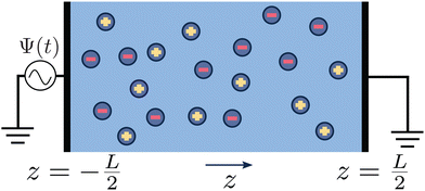 |
| | Fig. 1 Schematic representation of the aqueous 1:1 electrolyte of interest containing a continuum solvent and two ionic species confined between two parallel blocking electrodes separated by a distance L. The electrolyte is driven by a time-dependent electric potential Ψ(t) applied to the electrode at  while the other one at while the other one at  is kept grounded. is kept grounded. | |
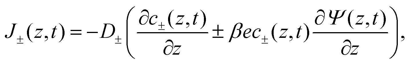
We use the Poisson–Nernst–Planck (PNP) equations to study the system. The first is the Poisson equation, which relates the local electric potential profile Ψ(z,t) to the local charge density e(c+(z,t) − c−(z,t)), where c±(z,t) denotes the concentration of cations (+) and anions (−) at position z and time t. For  the Poisson equation reads
| | 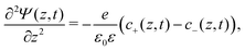 | (1) |
where
ε0 is the permittivity of vacuum and
ε = 80 represents water as a structureless continuum. The ionic fluxes
J±(
z,
t) contain a diffusive contribution due to the gradients of ion concentrations and a conductive contribution due to the potential gradient, jointly described by the Nernst–Planck equation
| | 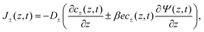 | (2) |
where we consider the diffusion coefficients to be spatially constant and different for cations (
D+) and anions (
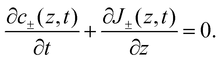
D−). Because we exclude any chemical reaction in the system, the concentrations and fluxes are coupled by the continuity equation
| | 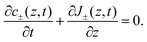 | (3) |
The PNP
eqn (1)–(3) form a closed set for the concentrations
c±, the fluxes
J± and the potential
Ψ. Solving PNP equations explicitly requires boundary and initial conditions, which we write as
| | | J±(−L/2,t) = J±(L/2,t) = 0, | (6) |
where
cs is the fixed initial average salt concentration, that is equal for both ionic species in our symmetric 1
:
1 electrolyte. Due to
eqn (3) combined with boundary conditions
eqn (6) the number of cations and anions will be conserved such that
| | 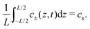 | (8) |
Here we note that for convenience during derivations below we use a complex representation of physical quantities (like for the voltage in
eqn (4)), however, in numerical calculations we use sin(
ωt) to drive the system (ensuring that the system starts from equilibrium with
Ψ(
z,0) = 0), therefore the physical quantities will correspond to the imaginary part of derived complex expressions. For given
Ψ0,
D±,
ω and
cs,
eqn (1)–(8) complete the system of non-linear coupled differential equations. We solve these equations numerically employing COMSOL® as a finite-element method solver software.
Convenient insight into relevant system parameters can be obtained as follows. In static equilibrium, so for ω = 0, the applied potential Ψ(−L/2,t) = Ψ0 (a constant), and J±(z,t) = 0, and in the linear regime with |βeΨ0| ≲ 1, the EDLs get fully developed at the two electrodes and the NP eqn (2) can be integrated to obtain the Boltzmann distribution
| | 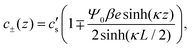 | (9) |
with
κ−1 the characteristic Debye length of the equilibrium EDL given by
| | 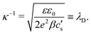 | (10) |
The concentration

is an integration constant that is very close to
cs in the large
L-limit of interest here, so throughout the paper we set

in the definition of
λD. In this limit, as we will derive below, the characteristic timescale of EDL formation
31,36 is written as the RC time
| | 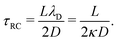 | (11) |
For future convenience we also define the Debye time
| | 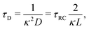 | (12) |
during which the ions diffuse over a distance of the order of the Debye length.
31,37 Here the effective diffusion coefficient of the ions in the electrolyte is given by
| |  | (13) |
For later reference it proves convenient to keep
D fixed and to characterise the asymmetry of
D+ and
D− by
| |  | (14) |
such that
| | 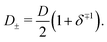 | (15) |
Clearly, for equal diffusivities we have
D =
D+ =
D−, however, for extremely asymmetric diffusivities the effective diffusion coefficient is essentially twice the smallest one.
For a few typical 1:1 electrolytes the asymmetry parameter δ is given in Table 1. Although close-to-symmetric electrolytes with δ ≃ 1 exist according to the table, others have some degree of mobility asymmetry up to δ ≃ 2 in the present examples. For simplicity we restrict attention to monovalent ions here, however we note that the mobility asymmetry of multivalent ions can be larger, for instance BeCl2 has δ = 3.44. Without loss of generality we choose δ > 1 throughout this study, such that the negative ions will be the faster ones, thus D− > D+.
Table 1 Ionic mobility ratio δ = D−/D+ for various common aqueous 1:1 electrolytes38
| Salt |
Ions |
D
+
|
D
−
|
δ
|
| CsCl |
Cs+, Cl− |
2.06 |
2.03 |
0.99 × 10⁻⁹ m2 s−1 |
| CsI |
Cs+, I− |
2.06 |
2.05 |
1.00 × 10⁻⁹ m2 s−1 |
| KCl |
K+, Cl− |
1.96 |
2.03 |
1.03 × 10⁻⁹ m2 s−1 |
| NaCl |
Na+, Cl− |
1.33 |
2.03 |
1.53 × 10⁻⁹ m2 s−1 |
| LiI |
Li+, I− |
1.03 |
2.05 |
1.99 × 10⁻⁹ m2 s−1 |
3 Asymmetric rectified electric field (AREF)
3.1 AREF description
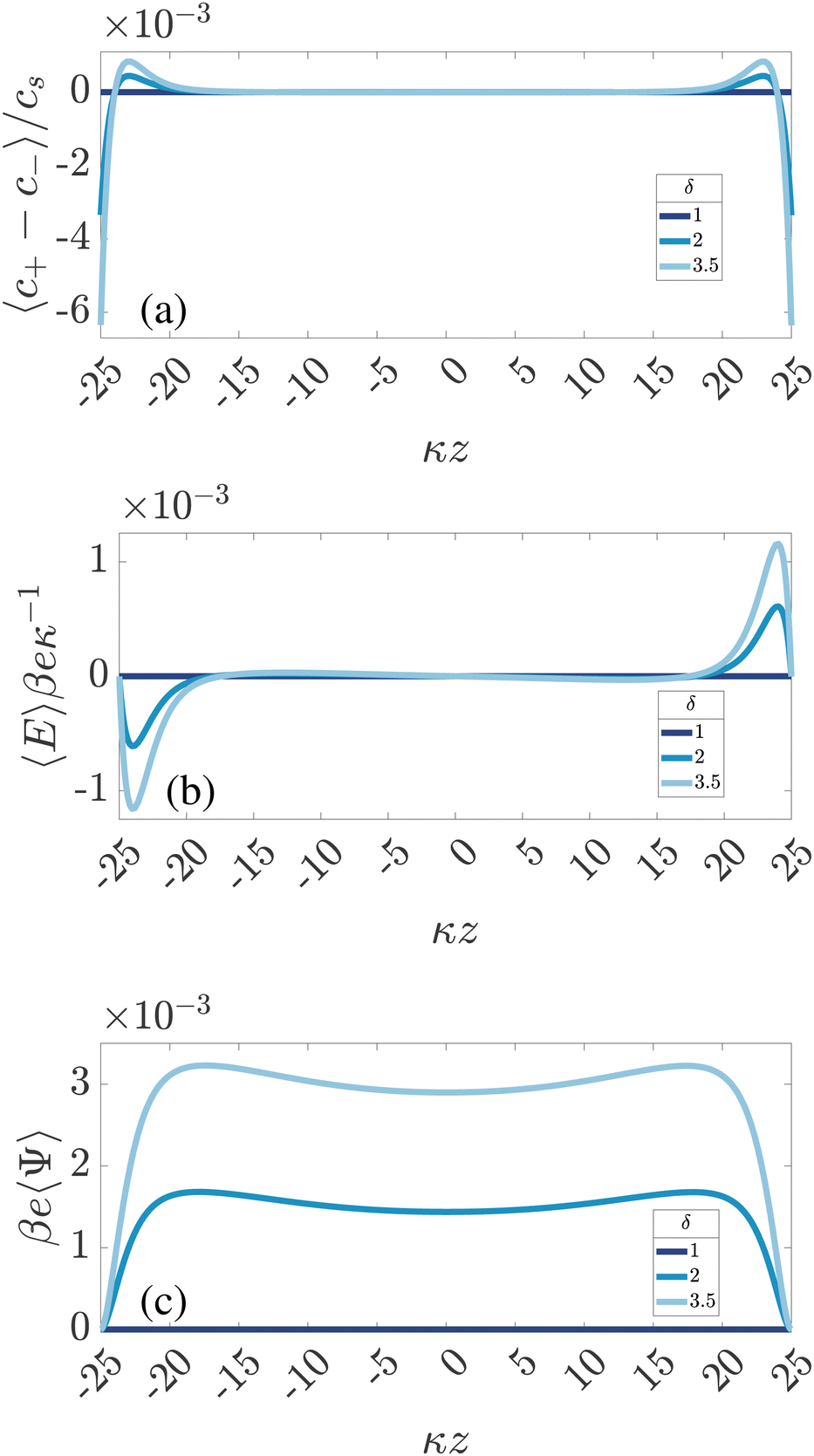
According to ref. 32, a mobility mismatch of ions, δ ≠ 1, can introduce a long-range steady electric field upon AC driving. This also follows from our numerical results. For convenience we define a standard parameter set including an amplitude and frequency of the driving potential given by βeΨ0 = 3 and ωτRC = 1, respectively. The standard system size is characterized by κL = 50, and the standard diffusion coefficients are D+ = D−/δ = 1.09 × 10⁻⁹ m2 s−1 (resulting in D = 1.456 × 10⁻⁹ m2 s−1) with δ = 2 by default. The bulk concentration of ions is cs = 1 mM, resulting in a Debye length λD = 10−8 m. Any deviation from this set will be explicitly stated. The coordinate z is measured in terms of Debye length λD = κ−1 and ranges from −L/2 to L/2. Our standard focus is also on the late-time limit-cycle when all transients have decayed such that all time-dependence has the same period as that of the driving potential, potentially, however, with higher-order harmonics.
In Fig. 2 we plot for the standard parameter set, with asymmetries δ = 1, 2 and 3.5, the late-time period-averaged position-dependent profiles of (a) the dimensionless charge distribution 〈c+ − c−〉 (z), (b) the electric field 〈E〉 (z), and (c) the potential 〈Ψ〉 (z). Here time-averaging is defined by
| | 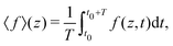 | (16) |
where
t0 is the (sufficiently late) time at which we start averaging,

is the period of AC voltage, and
f can be any of the functions that we are considering – either the electric field
E, the electric potential
Ψ, or a combination of the ion concentrations
c±.
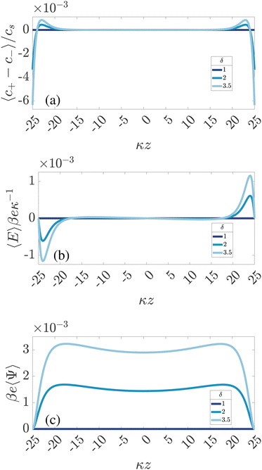 |
| | Fig. 2 Dimensionless spatial profiles of the time-averaged (a) ionic charge density 〈c+ − c−〉/cs, (b) electric field βeκ−1〈E〉, and (c) electric potential βe〈Ψ〉 for an aqueous 1:1 electrolyte with Debye length λD = 10 nm confined between two planar electrodes at distance L = 50λD. The electrode at z = L/2 is grounded, the one at z = −L/2 has an AC potential Ψ0eiωt with amplitude Ψ0 = 3/βe = 75 mV and frequency ω = τRC−1 with RC-time τRC given by eqn (11). The different colors represent the three different mobility ratios δ = D−/D+ of the faster anions and the slower cations. | |
For ω > 0, so for finite T, Fig. 2 shows for symmetric electrolytes (δ = 1) that 〈c+−c−〉 = 〈Ψ〉 = 〈E〉 = 0, meaning that charges are distributed evenly across the system, as expected. However, if the ionic mobilities become mismatched (δ = 2 and δ = 3.5), the average charge distribution 〈c+ − c−〉 becomes spatially non-uniform (see Fig. 2(a)), which, in turn, gives rise to a non-zero time-averaged electric field and a steady non-uniform electric potential, presented in Fig. 2(b) and (c), respectively. We note in Fig. 2(c) that the time-averaged electrode potential is zero by construction, as imposed by the boundary conditions. Nevertheless, the steady electric field extends several Debye lengths into the electrolyte (in the current case it is more than 5λD, however this can be even more, as demonstrated in ref. 34). Fig. 2 gives a first clue of the underlying physics, as we see that 〈c+ − c−〉 is negative in the vicinity of the surfaces and positive a few Debye lengths away, showing that the faster anions manage to approach the electrode in larger quantities, on average, than the slower cations.
Fig. 2(b) is an example of the long-range steady electric field that is referred to as Asymmetric Rectified Electric Field (AREF) in ref. 32. Parametric studies of AREF performed in ref. 34 concentrate on two characteristics of AREF – the position and the height of the largest peak of the concentration profile of the slower ions. Instead, here we use the spatio-temporal average U of the (dimensionless) electric potential profile to characterize the magnitude of AREF,
| |  | (17) |
which is a convenient integrated quantity to study numerically. Moreover, for large
L, the dimensionless quantity
U is a measure for the time-averaged electroosmotic (EO) mobility,
39 as it plays the same role as the zeta potential of charged surfaces; it is proportional to the physically measurable EO mobility
μEO. However, EO is not the focus of the current paper and can be explored in future studies. Finally, it is also interesting to note that the period-averaged surface charge density on the electrodes, 〈
σ〉 ∝ 〈
E|
z=−L/2〉 vanishes by Gauss law due to the electric neutrality of the system. This is also clear from
Fig. 2b, where the curves of 〈
E〉 approach zero at
z = ±
L/2. Thus the layers of fast anions that we see at each of the electrodes in
Fig. 2a essentially play the role of charged electrodes that are screened by the cloud of slow cations.
3.2 AREF mechanism
Here we discuss the mechanism for AREF generation. It is perhaps best understood by tracking the number of ions gathering at one of the electrodes (e.g. the one at z = −L/2) for the whole period T = 2π/ω. In the electrolytic cell that we are considering with the driving voltage given by eqn (4), in the first half of the period T/2 the negative (faster) ions will gather at the chosen electrode because it is positive, whereas in the second half the positive (slower) ones will tend to get closer. If the frequency of the voltage is such that the EDLs have enough time to develop (but not fully form) during the T/2 time span, the faster ions will manage to gather at the electrode in larger amounts. Therefore, if we average the number of ions at the electrode over the whole period T, we will get an excess of faster ions at the electrode. Exactly the same thing occurs at the opposite electrode, however with a T/2 shift in phase. This is what we also observe in Fig. 2(a), where the negative (faster) ions are accumulating at both electrodes on average in time. Moreover, due to the global electroneutrality of the cell, the surface charge on both electrodes is zero on average, such that the excess of the negative ions at both electrodes is screened by the excess of the oppositely charged ions located several Debye lengths away from the electrodes for the current parameters, as seen in Fig. 2(a).
4 Parameter dependence of AREF
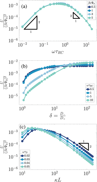
In this section we study the dependence of the numerically obtained AREF magnitude U on the main system parameters.
4.1 Applied voltage amplitude
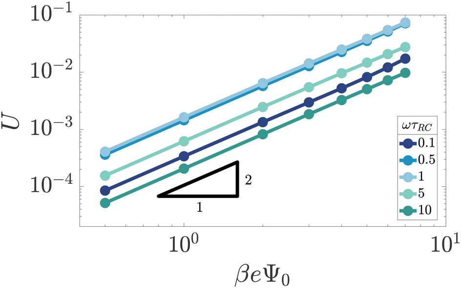
We start by studying the dependence of the space- and time-averaged potential U as defined in eqn (17) on the amplitude Ψ0 of the externally applied AC potential. The range that we consider for the driving voltage amplitude Ψ0 is limited from above by our point ion approximation, which for cs = 1 mM can become unrealistic due to strong ion crowding effects at the electrodes.40–42 This occurs beyond βeΨ0 ≈ 8, which is therefore the upper limit that we consider.
Fig. 3 shows the dependence of U on Ψ0 for various driving frequencies for our standard parameter set. For the full range of frequencies ωτRC ∈ [0.1,10] that we consider here, the slope of the double-logarithmic curves is essentially identical to 2, i.e. U ∼ Ψ02 for all frequencies considered, which is in line with the findings of ref. 34. It should be noted, however, as was also demonstrated in ref. 34, that the AREF scaling deviates somewhat from Ψ02 at even higher voltage amplitudes Ψ0 > 10. This voltage range leads, at least at low frequencies, to high ionic concentrations outside the regime of applicability of the underlying point-ion model. For this reason we leave this high-voltage regime out of the discussion in the current paper. In the regime of interest the scaling confirms that AREF is a non-linear screening effect and motivates the study of its dependence on frequency, mobility asymmetry, and system size in terms of the scaled form U/(βeΨ0)2 below.
 |
| | Fig. 3 Double-logarithmic representation of the period- and space-averaged dimensionless potential U of eqn (17) as a function of the driving voltage amplitude for varying driving frequencies ω at our standard parameter set (see text). The quadratic scaling U ∼ Ψ02 demonstrates that AREF is a non-linear effect. | |
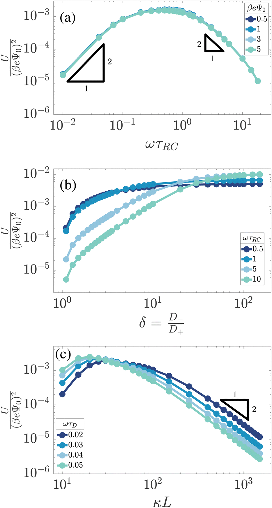
4.2 Frequency
Fig. 3 already showed that U is relatively large at ωτRC ≈ 1 and considerably smaller at ωτRC = 0.1 and 10. Here we study for several Ψ0 the frequency-dependence of U as obtained from the numerical solutions of the PNP equations in full detail for our standard parameter set. Fig. 4(a) shows U/(βeΨ0)2 as a function of ωτRC, featuring the expected collapse for all Ψ0, a broad maximum at ωτRC ∼ 1, and an algebraic decay ∼ω2 for small frequencies ω. For frequencies ω in the ωτRC ∼ 1–10 range, the curve shows an algebraic ∼ω−2 decay, however, as the frequency ω gets increased further, the slope of the curve becomes steeper (stronger decay) due to an overscreening effect that starts to appear at the electrodes in this regime.
 |
| | Fig. 4 Dimensionless and scaled period-averaged potential U/(βeΨ0)2 as obtained from numerical late-time solutions of the PNP equations for the standard parameter set (see text), in (a) as a function of the dimensionless frequency ωτRC, in (b) as a function of the the mobility asymmetry δ = D−/D+, and in (c) as a function of the dimensionless system size κL, in all three cases in a double-logarithmic representation. In (a) we see a collapse of the curves for several voltage amplitudes Ψ0. In (b) and (c) we consider several dimensionless frequencies ωτRC and ωτD, respectively. | |
Qualitatively this frequency dependence can be explained by the mechanism that we proposed above. In the low-frequency limit, the system is nearly static and during the time span T/2 both ion species have enough time to essentially fully build up an EDL at the corresponding electrodes. Thus the number of ions in this fully developed EDL is the same for both half periods, the average ionic charge and thus the potential at the electrodes in the timespan T approaches zero, which agrees with the low-frequency part of the curve in Fig. 4(a). In the high-frequency limit, on the other hand, none of the ion species, not even the faster ones, has enough time to develop the EDLs. Therefore no net accumulation of charge occurs at the electrodes, yielding a decaying trend for U as the frequency increases. The maximum of the effect is reached for intermediate frequencies of the order of the characteristic RC time for EDL formation ωτRC ∼ 1. At these frequencies the difference between the number of fast and slow ions gathering at the electrodes in the T/2 timespan is largest.
4.3 Ion mobility asymmetry
The asymmetry of ion mobility, δ ≠ 1, is the main cause of AREF and here we study how U depends on δ at fixed effective diffusion coefficient D-such that τRC remains fixed if we vary δ for fixed L and λD. For our standard parameter set Fig. 4(b) shows the δ-dependence of U/(βeΨ0)2 for several driving frequencies ωτRC. Here we extend the interval for δ ∈ [1,100] far beyond the typical range for small ions to identify that apart from the common monotonic increase of U with δ the curves are highly non-universal, with a frequency-dependent asymptotic saturation of U at high δ that is larger for higher frequencies whereas U is smaller for higher frequencies in the low-δ regime, with a crossover at δ ≃ 20–30.
These results can qualitatively be explained within the scope of our proposed mechanism, where the large-δ limit proves helpful. Let us consider a (late-time) period [t0,t0 + T] and divide it into two half periods in which the potential of the electrode at z = −L/2 is positive for t ∈ [t0,t0 + T/2] ≡ t+ and negative for the complementary interval t ∈ [t0 + T/2,t0 + T] ≡ t−. Introducing the maximum of the (absolute) areal ionic charge on this electrode during either of these periods as
| |  | (18) |
we expect, for
δ > 1, that
Γ− >
Γ+ since the faster anions can accumulate faster in
z ∈ [−
L/2,0] during
t− than the slower cations can during
t+ (for simplicity we ignore the fact that the faster anions also deplete faster than the slower cations, as depletion has a weaker contribution to the competition of number of ions present at the electrode compared to the accumulation).
Now let us assess how δ affects the charge accumulation process. From eqn (15) we see for increasing δ at fixed D that cations will asymptotically settle at a fixed diffusion coefficient  while the anions become increasingly mobile. At finite frequency, their finite mobility sets a limit for the amount of accumulation or depletion of cations at the electrode. For anions, despite the fact that their diffusion coefficient becomes increasingly faster, the equilibrium EDL configuration still imposes a limit to the anion concentration close to the electrode. Taking this into account, it becomes clear that
  which is exactly what we see in Fig. 4(b).
To explain the different saturation values of U in Fig. 4(b), we notice that at the low (realistic) values of δ the value of U follows the logic of the U(ω) curves – the maximum is achieved at around ωτRC ∼ 1. However, as we increase δ, the hierarchy of the curves changes and in the δ → ∞ limit U(δ) reaches higher values for higher frequencies ω. The number of charges contained in a fully developed EDL only depends on the thermodynamic properties of the electrolytic cell together with the magnitude of the applied voltage, therefore, in the δ→∞ limit anions will fully form an EDL irrespective of the (finite) voltage frequency ω. However, the concentration of cations gathered at the electrode-decreases with the frequency ω (as the higher the frequency ω, the less time there is for ions to gather), therefore the saturation value of U, proportional to the difference in the number of anions and cations gathered at the electrode, will increase with frequency, which is again exactly what we observe in Fig. 4(b).
4.4 System size
In Fig. 4(c) we plot U/(βeΨ0)2 as a function of the system size L (in units of the Debye length) for our standard parameter set at a number of dimensionless frequencies ωτD. Up to this point we used the dimensionless combination ωτRC of eqn (12) to characterize the frequency of the AC voltage, which, however, is not convenient here since τRC itself depends on the system size, according to eqn (11). For the system sizes κL∈ [10,103] that we consider here, we see that U peaks at larger κL for lower frequencies ωτD, which corresponds in fact to a peak in the regime where ωτRC ∼ 1, consistent with our earlier findings in Fig. 4(b). For κL ≫ 102 we observe an algebraic decay U ∝ L−2, the exponent of which resembles that of the decay U ∝ ω−2 that we found in Fig. 4(a). This similar decay is not surprising since the key dimensionless parameter ωτRC is linear in both L and ω. However, as we will see in Section 6.2, the reason for this quadratic algebraic decay U ∝ L−2 is a bit more subtle than it seems here.
5 Equivalent circuit from linearized PNP equations
An alternative way of studying the system of interest involves the construction of an equivalent RC circuit, rather than relying solely on the numerical calculations.16,43–46 This convenient strategy of studying electro-chemical systems has been employed in this field for many years; for a historical overview on this matter we refer the reader to ref. 47. In the present case we first construct an equivalent RC circuit corresponding to the electrolytic cell in Fig. 1 in the linear regime for which Ψ0 ≪ 1/βe – we will modify this model later to account for the intrinsically nonlinear character of AREF. In the linear regime, a widely used scheme is a simple RC circuit with R and C elements connected in series.30,31,48 However, as we will now show, it is not entirely accurate at high frequencies where ωτRC > 1.
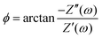
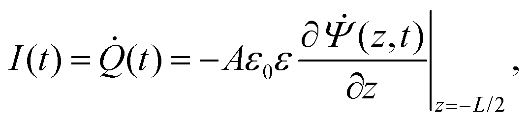
In order to determine an equivalent circuit for our model we study its frequency response using the electrical impedance defined as
| | 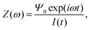 | (19) |
where
I(
t) is the current flowing through the external (electronic) system due to the applied potential over the electrodes. The current is the time derivative (indicated by a dot) of the charge
Q(
t) =
Aσ(
t) on the electrode at
z = −
L/2 and can be calculated from the time-dependent potential profile
Ψ(
z,
t) using Gauss' law as
| | 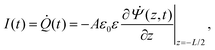 | (20) |
with
A the surface area of the electrode. Within the linear regime the PNP equations and boundary conditions of
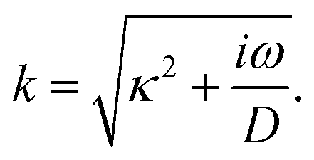
eqn (1)–(8) are well known to be solvable analytically, resulting in
| | 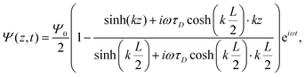 | (21) |
where we define the complex wavenumber
| |  | (22) |
Here
D is the effective diffusion coefficient introduced in
eqn (13).
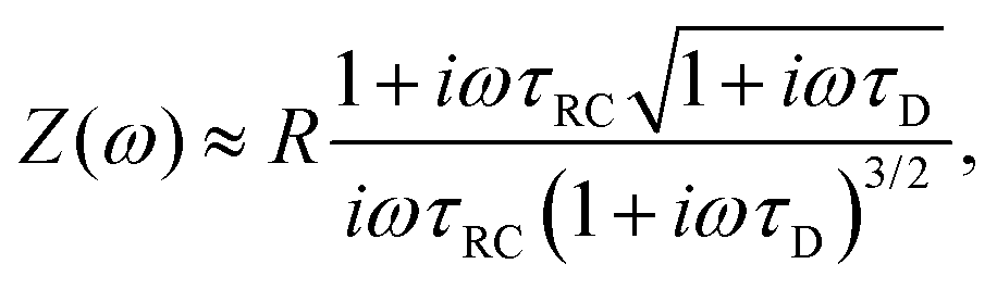
Inserting eqn (21) together with eqn (20) into eqn (19) and also assuming that the system is large, L ≫ κ−1, we obtain the explicit expression
| | 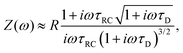 | (23) |
where
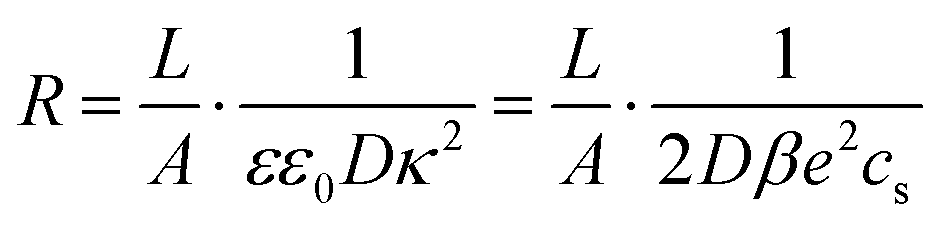
| |  | (24) |
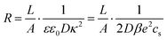
is the resistance of the system and
τRC, as defined in
(11), the timescale characterizing the EDL formation process. Note that
Z(
ω)/
R depends only on
ωτRC and
τRC/
τD =
κL/2.
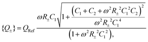
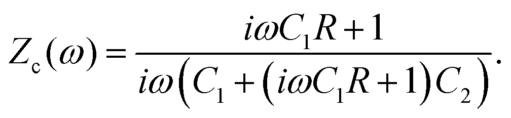
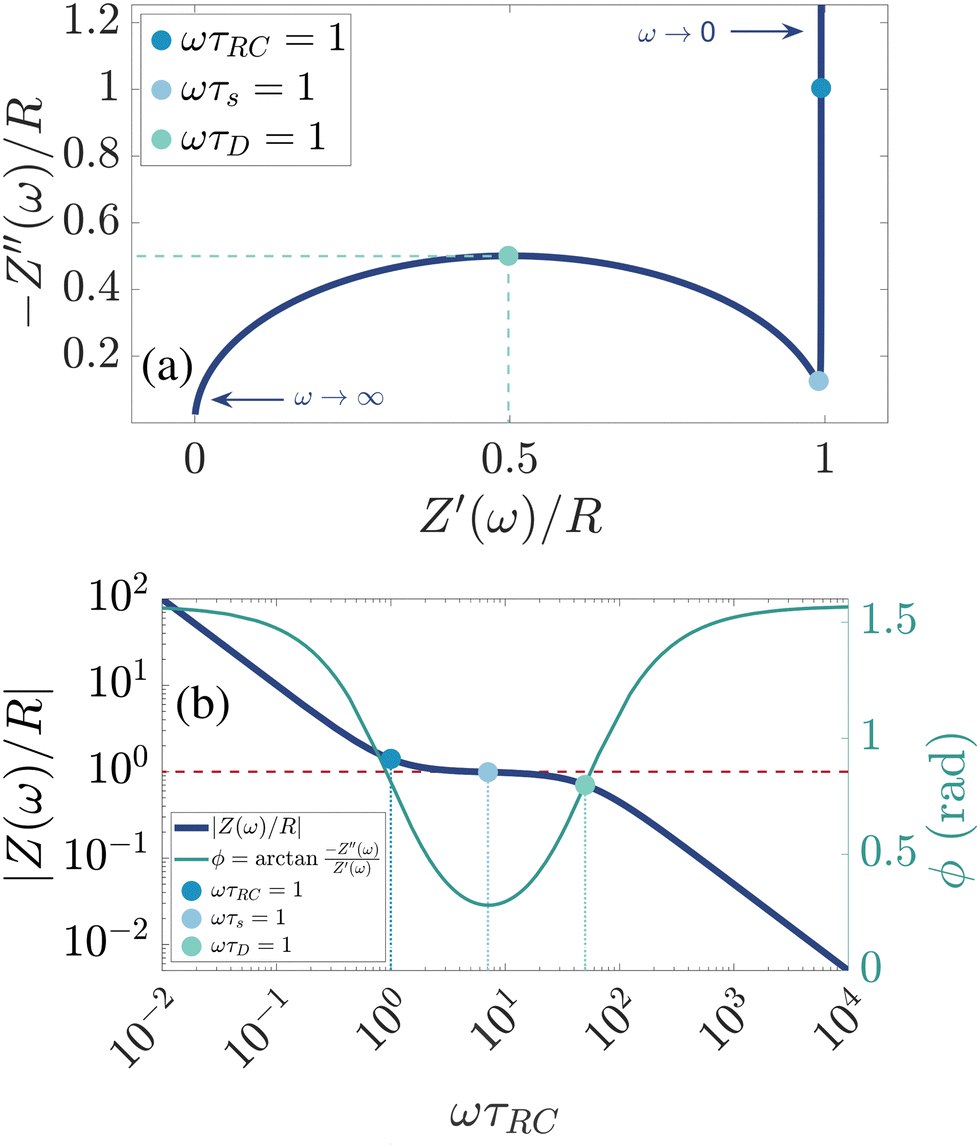
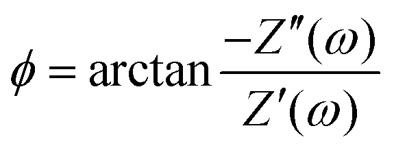
There are several ways to plot the frequency dependence of the impedance.13 We will use the so-called Argand complex plane diagrams for the complex impedance Z(ω) = Z′(ω) + iZ′′(ω), as represented by a parametric (ω dependent) plot of (Z′(ω), −Z′′(ω)). The Argand diagram will also be backed up with a Bode plot, describing how the impedance modulus |Z(ω)| depends on the frequency ω. The combination of Argand diagram together with a Bode plot often allows readily for an identification of a circuit, not only of the linear elements included in the circuit but also how they should be connected – either in series, parallel or combinations thereof. Usually the frequency response plots mentioned above are unique for relatively simple electric circuits.13 Nonetheless, in order to ensure the robustness of the chosen equivalent circuit configuration, it is a commonly employed strategy to support its selection with physical considerations. This ensures that the circuit mimics the behavior of the system it represents, as detailed in ref. 14. An electric circuit that produces similar Argand and Bode curves while also possessing a configuration consistent with physical principles is denoted as the equivalent electric circuit associated with the electrolytic cell.
We plot, for κL = 500, the Argand diagram of the dimensionless combination Z(ω)/R given by eqn (23) in Fig. 5(b) and the corresponding Bode plot in Fig. 5(b), in both cases with dots at three characteristic frequencies. The Argand diagram features a vertical line at Z′ = R in the low-frequency limit, characteristic for a resistor R with a capacitor connected in series, and a semi-circle with a maximum of −Z′′ = R/2 at Z′ = R/2 for higher frequencies, characteristic for a parallel connection of a resistor R and a capacitor. The Bode plot gives us similar clues, allowing us to identify the electric response of the electrolytic cell with that of an equivalent circuit that consists of a capacitor C2 in parallel with a resistor R and a capacitor C1 in series, as illustrated in Fig. 7(a). The impedance Zc(ω) corresponding to this circuit can easily be calculated and reads
| |  | (25) |
We note that the functional forms of
eqn (23) and (25) are actually slightly different, however with a remarkable agreement for our regime of interest where −
C1 ≫
C2, which translates into
κL ≫ 1 as we will discuss in more detail below. In order to derive the expressions for the individual elements
C1,
C2 and
R of the circuit, we match the impedances of the electrolytic cell and the circuit from
eqn (23) and (25), respectively, by considering the high- and low-frequency limits
ωτRC → ∞ and
ωτD → 0, respectively. For
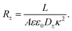
R this yields the bulk resistance of the electrolyte given by
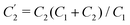
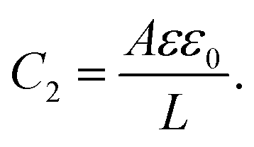
eqn (24) and for the capacitances we find
| |  | (26) |
| |  | (27) |
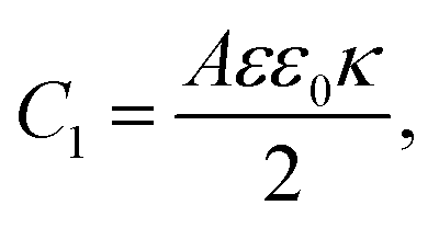
Physically
C1 corresponds to the net capacitance of the two fully developed EDLs in series,
i.e. at both planar electrodes, each with the linear-screening capacitance
Aεε0κ. Likewise,
C2 corresponds to the capacitance of a dielectric (water-filled) parallel-plate capacitor of size
L without any ionic charge carriers (and hence without any EDL).
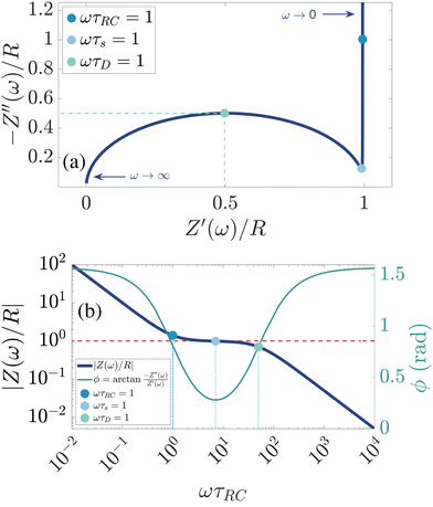 |
| | Fig. 5 (a) Argand diagram and (b) Bode plot characterising the frequency-dependence of the complex impedance of an electrolytic cell given by eqn (23), with system size κL = 500 for our standard parameter set (see text). Characteristic frequencies corresponding to the (long) RC-time τRC, the (short) Debye time τD, and the (intermediate) time  (see text) are indicated with dots. The Bode plot also features the frequency dependence of the phase shift, showing a minimum at ωτs = 1. (see text) are indicated with dots. The Bode plot also features the frequency dependence of the phase shift, showing a minimum at ωτs = 1. | |
We remarked already that the functional form of the impedances of the cell and the effective circuit are not identical. Using the matching parameters for R, C1, and C2 determined above, we compare in Fig. 6 the Argand plots of the cell (solid lines) and the electric circuit of Fig. 7(a) (dashed lines), for system sizes κL = 30, 100, and 1000. For all three system sizes the agreement is rather good for all frequencies, especially for high frequencies ωτD ≫ 1 where EDLs can hardly develop. For the two smaller systems sizes deviations between the solid and dashed lines can be seen by eye at higher frequencies, however their distinction is beyond the resolution of the plot for κL = 1000. This can be quantitatively appreciated by the inset of Fig. 6, where the maximum difference between unity and the ratios  and
and  , defined as
  and
and  are plotted as a function of system size κL. Here we denote the real and imaginary parts of the circuit impedance from eqn (25) by
  and
and  , respectively. The inset of Fig. 6 clearly shows an increasing agreement between the two frequency responses with increasing system size with differences decaying proportional to (κL)−1. Hence we can faithfully use the circuit in Fig. 7(a) to represent the electrolytic cell for κL ≫ 1.
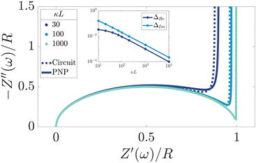 |
| | Fig. 6 Argand diagrams for the complex impedance of the electrolytic cell (solid lines) and the equivalent circuit (dashed lines) for system sizes κL = 30, 100, 1000 and our standard parameter set (see text). The inset shows the (small) maximum deviation of the ratios  and and  from unity as a function of system size κL, indicative of the increasingly good agreement between PNP calculations of the cell and the equivalent circuit for larger system sizes. from unity as a function of system size κL, indicative of the increasingly good agreement between PNP calculations of the cell and the equivalent circuit for larger system sizes. | |
 |
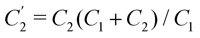
| | Fig. 7 (a) Equivalent electric circuit corresponding to the electrolytic cell in the linear regime for large system sizes L ≫ κ−1. (b) Alternative version of the equivalent circuit with modified elements (see text). (c) Simplified equivalent electric circuit corresponding to the low-frequency case 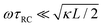 . Here R and C2 correspond to the resistance and capacitance of the cell at infinite frequency, respectively, and C1 is the total capacitance of two fully developed electric double layers at the electrodes, as described by eqn (24), (26), and (27). . Here R and C2 correspond to the resistance and capacitance of the cell at infinite frequency, respectively, and C1 is the total capacitance of two fully developed electric double layers at the electrodes, as described by eqn (24), (26), and (27). | |
Interestingly, the circuit of Fig. 7(b) can be shown to have an impedance of the exact same functional form as eqn (25), however with modified elements  ,
,  , and
, and 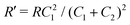 . This implies that the capacitor ratio of the two circuits is the same,
  , and also that
 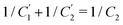 . Since the difference between the circuits becomes irrelevant in the limit C1 ≫ C2 of our main interest, we focus on the circuit of Fig. 7(a) in the remainder of this work.
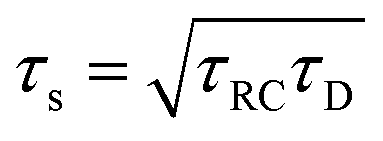
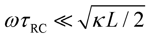
Let us return to the Argand diagram of Fig. 5(a), for which we already discussed the vertical line at sufficiently low frequencies, which implies that in this regime the equivalent circuit is the simple serial circuit shown in Fig. 7(c), with R and C1 in series without the second capacitor C2 in parallel. This simplified equivalent circuit has been used to model electric cells in many studies before,30,31,48,49 however the presence of the semi-circle shows that the simplified circuit breaks down at high enough driving frequencies. Interestingly, the crossover between the semi-circle and the vertical line, i.e. the crossover regime for the (un)importance of C2 in the equivalent circuit, does neither occur at frequencies as high as ω ≃ 1/τDnor at frequencies as low as ω ≃ 1/τRC, but rather at frequencies ω ≃τs−1 where we introduce the intermediate characteristic time scale
| | 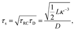 | (28) |
where the label s stands for “series”. The simplified series approximation shown in
Fig. 7(c) only holds for
ω ≲
τs−1. Physically,
τs characterises the timescale at which the imaginary part of the impedance (
i.e. the capacitive effects of the circuit) gets minimized. This is clearly visible in
Fig. 5(b), where the phase angle
is seen to exhibit a minimum for
ωτs ∼ 1.
We should note here though, that the presence of the additional τs and τD timescales does not influence the characteristic charging time of the full circuit and it matches that of an RC in series circuit. The reason for this is that we work with large systems κL ≫ 1 which translates into C1 ≫ C2, meaning that the total charging time will be dictated by how fast the C1 capacitor is charged.
6 Toy model
6.1 Modified linear circuit
Even though the mechanism of the AREF allows for a qualitative understanding of the numerical results of Section 4, a more quantitative explanation remains missing, for instance on the exponents characterising the algebraic decay of the time- and space-averaged potential U at high and low frequencies and the scaling with system size. For this reason we will now construct a simplified model of the electrolytic cell based on the equivalent circuit of Fig. 7(a). This model will allow us to analytically calculate a proxy of U, namely the period-averaged charge gathered in the EDL. As we will see below, in the majority of cases this charge has a similar dependence on the system parameters as U.
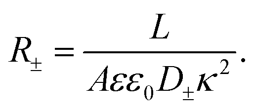
Clearly, however, due to the linear nature of the equivalent circuit, some modifications are needed to account for the intrinsically non-linear nature of AREF. For the clarity of explanation, we start by exploiting the mirror symmetry of the geometry to concentrate only on the left half of the system z ∈ [−L/2,0], as the right half z ∈ [0,L/2] will be in exact anti-phase. In our toy model we calibrate the time such that the electrode potential at z = −L/2 is positive during t ∈ [0,T/2] and negative during t ∈ [T/2,T], with T = 2π/ω the period. We assume that the EDL of the left electrode gets charged only by the fast anions in the first half of the period, while only the slow cations charge the same electrode in the second half of the period. This assumption significantly simplifies the treatment of the system, as it clearly separates the timescales of EDL charging/discharging processes by fast and slow ions, while allowing us to characterize the inherently non-linear charging process by combining two separate linear equivalent circuits albeit with different system parameters during the two half periods. Throughout we use the equivalent circuit of Fig. 7(a), however with two different ionic mobilities D±, and hence two different resistances R− for t ∈ [0,T/2] and R+ for t ∈ [T/2,T], which in analogy to eqn (24), are given by
| |  | (29) |
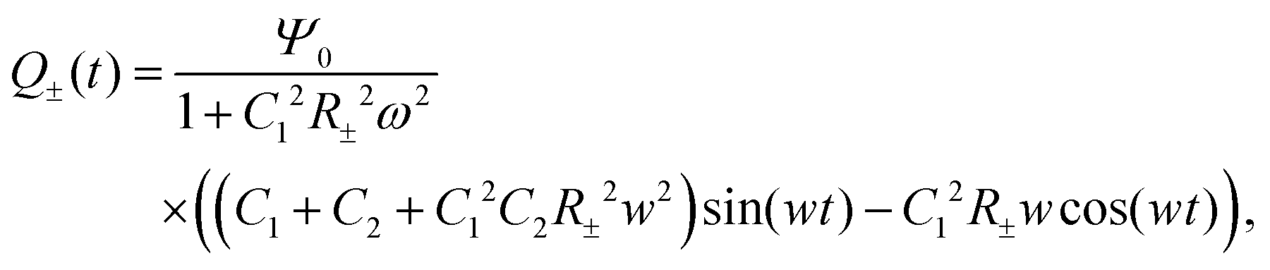
For Ψ(t) = Ψ0eiωt, by employing Kirchhoff's equation and Laplace transformation, it is straightforward to calculate the total electric charge Q±(t) on the two capacitors C1 and C2 for each of the two equivalent circuits, and we find
| |  | (30) |
where we neglected all the transient terms, as we are interested in the limit-cycle solutions. Here we note that
C1 and
C2 are thermodynamic quantities that do not depend on the ionic transport properties such as diffusion coefficient; they are given in
eqn (26) and (27) and are the same for both types of ions during each of the two half periods. For both sets of circuit parameters we can then calculate the average charge {
Q±} on the capacitors in the interval
t ∈ [
t0,
t0 +
T/2], yielding
| | 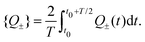 | (31) |
We now chose
t0 such that
Q±(
t) is positive for
t ∈ [
t0,
t0 +
T/2], which is always possible because
Q±(
t) of
(30) is a harmonic function with the same frequency as the driving voltage. Inserting
eqn (30) into
eqn (31) yields
| |  | (32) |
with a convenient reference charge defined by
QRef = (2/π)
C1Ψ0 that is identical in the circuits and the two half-periods. Following our convention that
D− >
D+ we can then calculate the dimensionless period-averaged net charge
| |  | (33) |
which is a measure for the time-averaged excess charge that is accumulated in a circuit with low resistance (corresponding to the fast anions charging an EDL at a positive electrode potential) compared to the circuit with a higher resistance (corresponding to the slower cations charging the EDL). Below we will consider
Q′ as a proxy for the space- and time-averaged potential
U of
eqn (17). Interestingly, one checks that
Q′ only depends on three dimensionless parameters that can be represented by
C1/
C2,
R+/
R−, and
which are equal to the system size
κL, the mobility asymmetry
δ, and
ωτRC, respectively. These three parameters correspond exactly to three of the four parameters on which
U depends, the fourth one being the amplitude of the driving potential
βeΨ0. The disagreement between the nonlinear dependence
U ∝
Ψ02 that we identified earlier and the independence of
Q′ on
Ψ0 is the price we pay for analysing the nonlinear AREF phenomenon in terms of linear-circuit theory. The dependence of
Q′ on
κL,
δ, and
ωτRC will, however, be quite similar to the dependence of
U on these parameters, as we will discuss now.
6.2 Parameter dependence of the proxy Q′
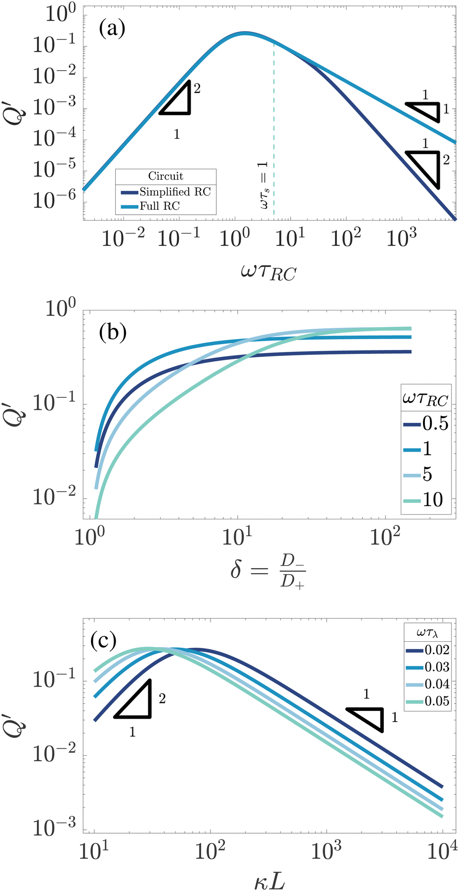
In Section 4 we studied the dependence of U on several system parameters numerically, using a standard reference set. Here we study to what extent the analytical expression of eqn (33) for the proxy Q′ gives similar results, where we use the same standard parameter set.
First we study the frequency dependence. In Fig. 8(a) we plot Q′ as a function of ωτRC, not only for the full RC-circuit of Fig. 8(b) but for comparison also for the simplified circuit of Fig. 4(a), for which C2 = 0 as in an infinitely large system with κL → ∞. It is apparent that for low to medium frequencies ω ≲ τs−1, as indicated by the vertical dashed line, both curves are strikingly similar to each other and to the one for U in Fig. 4(a), as all three share a broad maximum at ωτRC ∼ 1 and an algebraic decay ∝ω2 for small frequencies. However, at higher frequencies ωτRC ≫ 1 Fig. 8(a) shows a remarkable difference between the simplified and the full circuit, the former showing a decay Q′ ∝ ω−1 and the latter a decay Q′ ∝ ω−2. This can be attributed to C2 acting increasingly similar to a short circuit or a wire as we increase the frequency. Hence, the high-frequency scaling of Q′ of the full circuit is clearly closer to that of U, although the phenomenon of overscreening (that is obviously not included in the linear-circuit theory) causes deviations of the algebraic high-frequency scaling of U that is not included in Q′. Nevertheless, the overall agreement of the frequency dependence of U and Q′ is comforting and supports our view of the underlying mechanism. From this point onward we will only use results based on the full circuit that includes both a finite C1 and C2.
 |
| | Fig. 8 Dependence of the analytically calculated period-averaged charge difference Q′ given by eqn (33) for our standard parameter set (see text) on (a) the dimensionless frequency ωτRC, (b) the asymmetry of ionic mobilities  and (c) system size κL. In (a) Q′ is plotted for the full equivalent RC circuit of Fig. 7(a) and for the simplified one of Fig. 7(c). In (b) Q′ is plotted for several driving frequencies ω. The effective diffusion coefficient D, and, consequently, the frequency ω, is kept fixed along each curve. In (c) Q′ is plotted for several driving frequencies ω. Both (b) and (c) are based on the full equivalent circuit. and (c) system size κL. In (a) Q′ is plotted for the full equivalent RC circuit of Fig. 7(a) and for the simplified one of Fig. 7(c). In (b) Q′ is plotted for several driving frequencies ω. The effective diffusion coefficient D, and, consequently, the frequency ω, is kept fixed along each curve. In (c) Q′ is plotted for several driving frequencies ω. Both (b) and (c) are based on the full equivalent circuit. | |
Next we study the δ-dependence of Q′ for exactly the same parameters as we used for U in Fig. 4(b), i.e. for our standard parameter set with a fixed τRC. The resulting Q′ is plotted in Fig. 8(b) for δ ∈ [1,100] for various driving frequencies ωτRC. As was the case for U, we see that Q′ is monotonically growing with δ until an asymptotic large-δ limit that is larger for the higher frequencies than for the lower frequencies, which is the exact opposite of the ordering of Q′ in the small-δ regime. Hence we see once again that our modified linear circuits can catch some of the essential features of AREF.
Finally, we study the system-size dependence of Q′ by plotting it in Fig. 8(c) as a function of κL for several frequencies characterised by fixed ωτD, again for the same parameters as we used for U in Fig. 4(c). We can see that Q′ peaks at system sizes that vary from κL ≃ 20 at the highest frequency to κL ≃ 100 at the lowest frequency, which corresponds, for every frequency considered, to a peak at that system size where ωτRC ≃ 1. This is very similar to our finding for the L-dependence of U in Fig. 4(c). However, a key difference between Q′ and U involves their large-L scaling behaviour, which is seen to be given by Q′ ∝ L−1 in Fig. 8(c) whereas we found U ∝ L−2 in Fig. 4(c). As we mentioned earlier, changing the system size affects the electrolytic cell in a similar way as changing the driving frequency ω. However, in contrast to changing ω, which leaves the geometrical characteristics of the electrolytic cell and, correspondingly, those of the elements of the equivalent circuit unaffected, they change when κL is increased. At larger system sizes κL ≳ 100, the impedance corresponding to C2 grows and effectively closes the C2 branch of the full circuit for the current, turning it into a simplified circuit of Fig. 8(c). This in turn implies that the scaling of Q′ with L should be the same as with ω in the case of a simplified circuit i.e. it should decay as L−1, which is exactly what we see in Fig. 7(c). The reason why we saw the decay U ∝ L−2 in the PNP case is that increasing the system size of the electrolytic cell not only reduces C2 to negligible magnitude for large κL, but also linearly decreases the applied electric field at fixed Ψ0, which together result in U ∝ L−2 rather than U ∝ L−1.
We can conclude that the modified linear-circuit model captures quite a few of aspects of the numerical PNP results of the AREF. The toy model essentially suggests that the key ions are the ones closest to the electrode (anions in one half of the period and cations in the other half). The time-averaged result is dominated by the faster anions.
7 Summary and discussion
We studied the static time-averaged electric field that arises in the AC-driven electrolytic cell shown in Fig. 1 if the cations and anions have unequal diffusion coefficients D+ < D−. We solved the governing non-linear coupled Poisson–Nernst–Planck (PNP) equations numerically to study how the magnitude of this so-called asymmetric rectified electric field (AREF) depends on the main system parameters such as the amplitude of the applied AC voltage Ψ0, the driving frequency ω, the ionic mobility asymmetry δ, and the system size L. We also solved the linearized PNP equations analytically and constructed an equivalent RC-circuit for the electrolytic cell. Based on this circuit, which involves a capacitor C2 in parallel with a series of a restistor R and a capacitor C1, we propose a modification that serves as our toy model to describe and explain the physical mechanisms responsible for the nonlinear AREF effect in terms of linear circuits. The key is to consider two different resistances (R+ and R− associated with the different diffusion coefficients D+ and D− of the cations and the anions, respectively) during different phases of the driving voltage, with cations/anions dominating the oscillating dynamics at negative/positive electrode potentials.
Let us for comparison briefly mention an appealing alternative toy model for AREF, proposed in ref. 32, in which the key idea is to consider two point charges that oscillate in anti-phase with different amplitudes to mimic the AC driving of a (monovalent) cation and anion with different mobilities. Interestingly, the motion of these two ions is shown to create a non-zero time-averaged electric field far from the oscillation origin, which is then considered to be the analogue of AREF. While this picture is very appealing at first sight and seems to capture the essential AREF physics, it would actually only apply to a one-dimensional line of ions that connect the electrodes and that interact with three-dimensional “1/r” Coulomb potentials. In the geometry of interest here, however, the analogue would be oscillating three-dimensional planes of charge, which by Gauss law interact by one-dimensional Coulomb potentials “|z − z′|” such that both species produce a spatially constant but oppositely directed electric field that exactly cancels in a globally neutral system. So despite its attractive appeal its predicted AREF is strongly affected by the geometry of three-dimensional space.
The modified linear-circuit toy model proposed here, which is based on the (dis-)charging of 3D capacitive EDLs in planar geometry, also has some shortcomings. Nevertheless, it describes the scaling of the AREF magnitude with several important system parameters quite well and reveals the physical mechanism behind AREF generation. The asymmetry in the ion mobilities introduces an asymmetry in the speed of the charging process of the EDLs during the two half periods of negative and positive electrode potentials. At driving frequencies ω of the order of the characteristic charging time of EDLs in the system, ωτRC ∼ 1, the asymmetry causes a time-averaged ionic charge distribution where the faster ions are on average closer to the electrode and play the role of the surface charge in conventional EDLs, while the slower ones play the role of the screening cloud. This results in a non-zero time-averaged EDL-like AREF structure. Even though AREF is essentially a non-linear screening phenomenon, we could gain some additional insight from a linearized RC-circuit analysis where we considered the resistance R to take different values R+ ∝ D+−1 and R− ∝ D−−1 during different phases of the AC-potential. Interestingly, our circuit analysis also yields a new time scale  which implies the peculiar scaling τs ∝ L1/2 for a given electrolyte. This time scale involves a key role for the dielectric capacitor C2, even in the large-L regime of interest where the EDL capacitor C1 = κLC2 ≫ C2. Physically τs corresponds to the timescale that separates the low-frequency regime from the high-frequency one. When ωτs = 1 the phase angle of the current in the full electric circuit (see Fig. 7(a) has a minimum). While C2 might be safely set to zero at correspondingly low frequencies ωτs ≲ 1, it becomes increasingly important at higher frequencies. The timescale τs therefore also defines the threshold between the regimes in which the system can be treated as the simple RC circuit in series of Fig. 7(a) at low frequencies ωτs ≪ 1 and the full circuit of Fig. 7(a) at high frequencies ωτs ≫ 1.
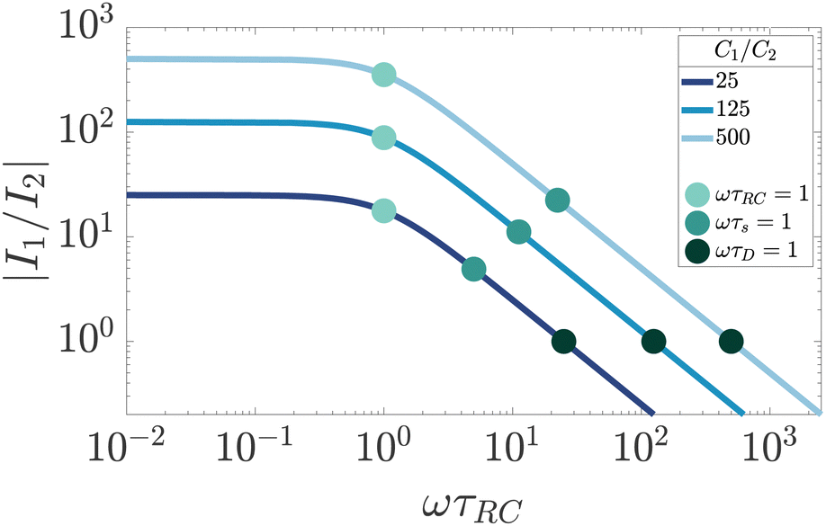
Finally, by studying the currents in the full electric circuit of Fig. 7(a) as shown in Fig. 9, we can also give the Debye time τD an additional physical interpretation. The currents in the C1 and C2 branches of the circuit of Fig. 7(a) become approximately equal in magnitude when ωτD = 1 (for κL ≫ 1). This means that τD corresponds to a timescale, at which the EDLs are built to such an extent that the combined impedance of the EDL capacitance and the bulk resistance of the cell becomes equal to that of the capacitor created by the electrodes of the cell.
 |
| | Fig. 9 Dependence of the ratio of electric current magnitudes |I1/I2| in the RC1 and C2 branches of the full circuit on the driving frequency ω, for various ratios of C1/C2 for our standard parameter set (see text). We clearly see that the currents have equal magnitude I1 = I2 for ωτD = 1, independently of the ratio C1/C2. | |
Extensions of our work could possibly involve the inclusion of redox or acid–base reactions, which would give additional time scales because of the reaction rates. Other directions could involve AC-electroosmosis or non-sinusoidal sawtooth-like potentials that break the symmetry between charging and discharging, in fact even for electrolytes with equal mobilities of the cations and anions. We speculate that amplification or suppression of the AREF effect is possible by tuning the combination of electrolyte, surface chemistry, and driving potential.
Conflicts of interest
There are no conflicts of interest to declare.
Acknowledgements
This work is part of the D-ITP consortium, a program of the Netherlands Organisation for Scientific Research (NWO) that is funded by the Dutch Ministry of Education, Culture and Science (OCW).
References
- M. M. Gregersen, L. H. Olesen, A. Brask, M. F. Hansen and H. Bruus, Phys. Rev. E: Stat., Nonlinear, Soft Matter Phys., 2007, 76, 056305 CrossRef PubMed.
- A. Ajdari, Phys. Rev. E: Stat., Nonlinear, Soft Matter Phys., 2000, 61, R45 CrossRef CAS PubMed.
- S. S. Dukhin, Adv. Colloid Interface Sci., 1991, 35, 173–196 CrossRef CAS.
- A. Ramos, H. Morgan, N. G. Green and A. Castellanos, J. Colloid Interface Sci., 1999, 217, 420–422 CrossRef CAS PubMed.
- V. Studer, A. Pépin, Y. Chen and A. Ajdari, Analyst, 2004, 129, 944–949 RSC.
- J. Catalano and P. Biesheuvel, Europhys. Lett., 2018, 123, 58006 CrossRef.
- T. Woehl, B. Chen, K. Heatley, N. Talken, S. Bukosky, C. Dutcher and W. Ristenpart, Phys. Rev. X, 2015, 5, 011023 Search PubMed.
- S. C. Bukosky and W. D. Ristenpart, Langmuir, 2015, 31, 9742–9747 CrossRef CAS PubMed.
- W. Ristenpart, I. A. Aksay and D. Saville, Phys. Rev. Lett., 2003, 90, 128303 CrossRef CAS PubMed.
- P. Biesheuvel, Y. Fu and M. Bazant, Russ. J. Electrochem., 2012, 48, 580–592 CrossRef CAS.
- A. Campione, L. Gurreri, M. Ciofalo, G. Micale, A. Tamburini and A. Cipollina, Desalination, 2018, 434, 121–160 CrossRef CAS.
- S. Al-Amshawee, M. Y. B. M. Yunus, A. A. M. Azoddein, D. G. Hassell, I. H. Dakhil and H. A. Hasan, Chem. Eng. J., 2020, 380, 122231 CrossRef CAS.
-
A. Lasia, Modern aspects of electrochemistry, Springer, 2002, pp. 143–248 Search PubMed.
- M. E. Orazem and B. Tribollet, New Jersey, 2008, 1, 383–389 Search PubMed.
- Y. Solomentsev, M. Böhmer and J. L. Anderson, Langmuir, 1997, 13, 6058–6068 CrossRef CAS.
- K. S. Cole and R. H. Cole, J. Chem. Phys., 1941, 9, 341–351 CrossRef CAS.
- H. Fröhlich and A. Maradudin, Phys. Today, 1959, 12, 40–42 CrossRef.
-
P. Robin, T. Emmerich, A. Niguès, A. Siria, L. Bocquet, A. Ismail, A. Keerthi, A. Geim and R. Boya, APS March Meeting Abstracts, 2022, pp. Q02–012 Search PubMed.
- P. Robin, T. Emmerich, A. Ismail, A. Niguès, Y. You, G.-H. Nam, A. Keerthi, A. Siria, A. Geim and B. Radha,
et al.
, Science, 2023, 379, 161–167 CrossRef CAS PubMed.
- T. Kamsma, W. Boon, T. ter Rele, C. Spitoni and R. van Roij, Phys. Rev. Lett., 2023, 130, 268401 CrossRef CAS PubMed.
- S. Tada, T. Natsuya, A. Tsukamoto and Y. Santo, Biorheology, 2013, 50, 283–303 Search PubMed.
- J.-H. Lim, S. D. McCullen, J. A. Piedrahita, E. G. Loboa and N. J. Olby, Cell. Reprogram., 2013, 15, 405–412 CrossRef CAS PubMed.
- H. Helmholtz, Ann. Phys., 1879, 243, 337–382 CrossRef.
- A. Hashemi, G. H. Miller, K. J. Bishop and W. D. Ristenpart, Soft Matter, 2020, 16, 7052–7062 RSC.
- B. Balu and A. S. Khair, J. Eng. Math., 2021, 129, 4 CrossRef.
- A. Torres, R. van Roij and G. Téllez, J. Colloid Interface Sci., 2006, 301, 176–183 CrossRef CAS PubMed.
- A. Hollingsworth and D. Saville, J. Colloid Interface Sci., 2003, 257, 65–76 CrossRef CAS PubMed.
- C. Mangelsdorf and L. White, J. Chem. Soc., Faraday Trans., 1997, 93, 3145–3154 RSC.
- E. H. DeLacey and L. R. White, J. Chem. Soc., Faraday Trans. 2, 1981, 77, 2007–2039 RSC.
- L. H. Olesen, M. Z. Bazant and H. Bruus, Phys. Rev. E: Stat., Nonlinear, Soft Matter Phys., 2010, 82, 011501 CrossRef PubMed.
- M. Z. Bazant, K. Thornton and A. Ajdari, Phys. Rev. E: Stat., Nonlinear, Soft Matter Phys., 2004, 70, 021506 CrossRef PubMed.
- A. Hashemi, S. C. Bukosky, S. P. Rader, W. D. Ristenpart and G. H. Miller, Phys. Rev. Lett., 2018, 121, 185504 CrossRef PubMed.
- A. Hashemi, G. H. Miller and W. D. Ristenpart, Phys. Rev. Fluids, 2020, 5, 013702 CrossRef.
- A. Hashemi, G. H. Miller and W. D. Ristenpart, Phys. Rev. E, 2019, 99, 062603 CrossRef PubMed.
- X. Chen, X. Chen, Y. Peng, L. Zhu and W. Wang, Langmuir, 2023, 39, 6932–6945 CrossRef CAS PubMed.
- M. Janssen and M. Bier, Phys. Rev. E, 2018, 97, 052616 CrossRef CAS PubMed.
- I. Rubinstein, B. Zaltzman, A. Futerman, V. Gitis and V. Nikonenko, Phys. Rev. E: Stat., Nonlinear, Soft Matter Phys., 2009, 79, 021506 CrossRef CAS PubMed.
- Table of Diffusion Coefficients, https://www.aqion.de/site/diffusion-coefficients, Accessed: 17th November 2022.
- J. J. Bikerman, Z. Phys. Chem., 1933, 163A, 378–394 CrossRef.
- M. S. Kilic, M. Z. Bazant and A. Ajdari, Phys. Rev. E: Stat., Nonlinear, Soft Matter Phys., 2007, 75, 021503 CrossRef PubMed.
- M. V. Fedorov and A. A. Kornyshev, Electrochim. Acta, 2008, 53, 6835–6840 CrossRef CAS.
- M. Z. Bazant, M. S. Kilic, B. D. Storey and A. Ajdari, Adv. Colloid Interface Sci., 2009, 152, 48–88 CrossRef CAS PubMed.
- J. R. Macdonald, Phys. Rev., 1953, 92, 4 CrossRef CAS.
- J. R. Macdonald, J. Chem. Phys., 1971, 54, 2026–2050 CrossRef CAS.
- G. Barker, J. Electroanal. Chem., 1966, 12, 495–503 CAS.
- M. S. Abouzari, F. Berkemeier, G. Schmitz and D. Wilmer, Solid State Ionics, 2009, 180, 922–927 CrossRef.
- L. Geddes, Ann. Biomed. Eng., 1997, 25, 1–14 CrossRef CAS PubMed.
- J. R. Macdonald, J. Chem. Phys., 1954, 22, 1857–1866 CrossRef CAS.
-
R. Kortschot, PhD thesis, University Utrecht, 2014.
|
| This journal is © The Royal Society of Chemistry 2024 |
Click here to see how this site uses Cookies. View our privacy policy here. 
 Open Access Article
 This Open Access Article is licensed under a
  * and
R.
van Roij
* and
R.
van Roij
 whereas the right one, placed at
  is kept grounded. Here ω is the imposed angular frequency and Ψ0 the amplitude. A schematic representation of the system is shown in Fig. 1.

 while the other one at
  is kept grounded.
 the Poisson equation reads


 is an integration constant that is very close to cs in the large L-limit of interest here, so throughout the paper we set
  in the definition of λD. In this limit, as we will derive below, the characteristic timescale of EDL formation31,36 is written as the RC time
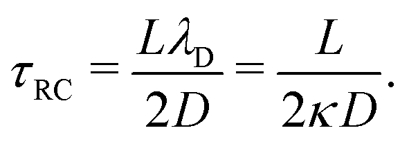


 is the period of AC voltage, and f can be any of the functions that we are considering – either the electric field E, the electric potential Ψ, or a combination of the ion concentrations c±.

 while the anions become increasingly mobile. At finite frequency, their finite mobility sets a limit for the amount of accumulation or depletion of cations at the electrode. For anions, despite the fact that their diffusion coefficient becomes increasingly faster, the equilibrium EDL configuration still imposes a limit to the anion concentration close to the electrode. Taking this into account, it becomes clear that
 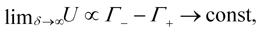 which is exactly what we see in Fig. 4(b).
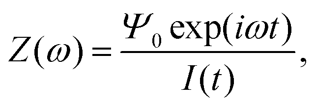

 (see text) are indicated with dots. The Bode plot also features the frequency dependence of the phase shift, showing a minimum at ωτs = 1.
 and
and  , defined as
 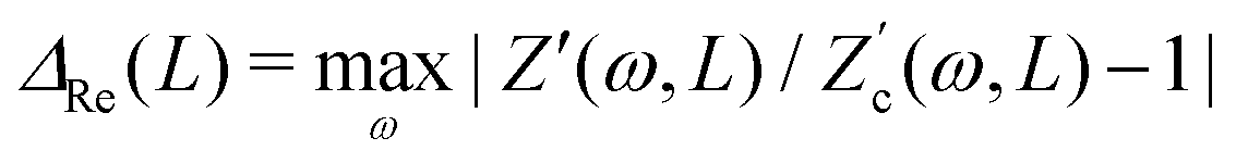 and
and 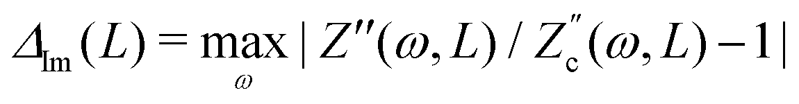 are plotted as a function of system size κL. Here we denote the real and imaginary parts of the circuit impedance from eqn (25) by
  and
and  , respectively. The inset of Fig. 6 clearly shows an increasing agreement between the two frequency responses with increasing system size with differences decaying proportional to (κL)−1. Hence we can faithfully use the circuit in Fig. 7(a) to represent the electrolytic cell for κL ≫ 1.
 and
and  from unity as a function of system size κL, indicative of the increasingly good agreement between PNP calculations of the cell and the equivalent circuit for larger system sizes.
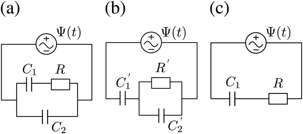
 . Here R and C2 correspond to the resistance and capacitance of the cell at infinite frequency, respectively, and C1 is the total capacitance of two fully developed electric double layers at the electrodes, as described by eqn (24), (26), and (27).
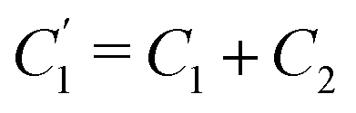 ,
,  , and
, and 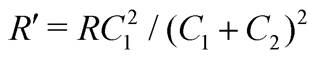 . This implies that the capacitor ratio of the two circuits is the same,
  , and also that
 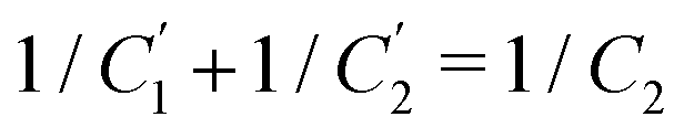 . Since the difference between the circuits becomes irrelevant in the limit C1 ≫ C2 of our main interest, we focus on the circuit of Fig. 7(a) in the remainder of this work.
 is seen to exhibit a minimum for ωτs ∼ 1.
 which are equal to the system size κL, the mobility asymmetry δ, and ωτRC, respectively. These three parameters correspond exactly to three of the four parameters on which U depends, the fourth one being the amplitude of the driving potential βeΨ0. The disagreement between the nonlinear dependence U ∝ Ψ02 that we identified earlier and the independence of Q′ on Ψ0 is the price we pay for analysing the nonlinear AREF phenomenon in terms of linear-circuit theory. The dependence of Q′ on κL, δ, and ωτRC will, however, be quite similar to the dependence of U on these parameters, as we will discuss now.
 and (c) system size κL. In (a) Q′ is plotted for the full equivalent RC circuit of Fig. 7(a) and for the simplified one of Fig. 7(c). In (b) Q′ is plotted for several driving frequencies ω. The effective diffusion coefficient D, and, consequently, the frequency ω, is kept fixed along each curve. In (c) Q′ is plotted for several driving frequencies ω. Both (b) and (c) are based on the full equivalent circuit.
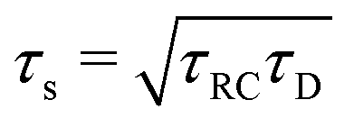 which implies the peculiar scaling τs ∝ L1/2 for a given electrolyte. This time scale involves a key role for the dielectric capacitor C2, even in the large-L regime of interest where the EDL capacitor C1 = κLC2 ≫ C2. Physically τs corresponds to the timescale that separates the low-frequency regime from the high-frequency one. When ωτs = 1 the phase angle of the current in the full electric circuit (see Fig. 7(a) has a minimum). While C2 might be safely set to zero at correspondingly low frequencies ωτs ≲ 1, it becomes increasingly important at higher frequencies. The timescale τs therefore also defines the threshold between the regimes in which the system can be treated as the simple RC circuit in series of Fig. 7(a) at low frequencies ωτs ≪ 1 and the full circuit of Fig. 7(a) at high frequencies ωτs ≫ 1.