
 Open Access Article
 This Open Access Article is licensed under a
 Creative Commons Attribution 3.0 Unported Licence
Understanding Cu(I) local environments in MOFs via63/65Cu NMR spectroscopy†
Wanli
Zhang
a,
Bryan E. G.
Lucier
 a,
Victor V.
Terskikh
b,
Shoushun
Chen
c and
Yining
Huang
*a
a,
Victor V.
Terskikh
b,
Shoushun
Chen
c and
Yining
Huang
*a
aDepartment of Chemistry, The University of Western Ontario, 1151 Richmond Street, London, Ontario N6A 5B7, Canada. E-mail: yhuang@uwo.ca
bMetrology, National Research Council Canada, Ottawa, Ontario K1A 0R6, Canada
cCollege of Chemistry and Chemical Engineering, Lanzhou University, Lanzhou 730000, China
First published on 27th February 2024
Abstract
The field of metal–organic frameworks (MOFs) includes a vast number of hybrid organic and inorganic porous materials with wide-ranging applications. In particular, the Cu(I) ion exhibits rich coordination chemistry in MOFs and can exist in two-, three-, and four-coordinate environments, which gives rise to many structural motifs and potential applications. Direct characterization of the structurally and chemically important Cu(I) local environments is essential for understanding the sources of specific MOF properties. For the first time, 63/65Cu solid-state NMR has been used to investigate a variety of Cu(I) sites and local coordination geometries in Cu MOFs. This approach is a sensitive probe of the local Cu environment, particularly when combined with density functional theory calculations. A wide range of structurally-dependent 63/65Cu NMR parameters have been observed, including 65Cu quadrupolar coupling constants ranging from 18.8 to 74.8 MHz. Using the data from this and prior studies, a correlation between Cu quadrupolar coupling constants, Cu coordination number, and local Cu coordination geometry has been established. Links between DFT-calculated and experimental Cu NMR parameters are also presented. Several case studies illustrate the feasibility of 63/65Cu NMR for investigating and resolving inequivalent Cu sites, monitoring MOF phase changes, interrogating the Cu oxidation number, and characterizing the product of a MOF chemical reaction involving Cu(II) reduction to Cu(I). A convenient avenue to acquire accurate 65Cu NMR spectra and NMR parameters from Cu(I) MOFs at a widely accessible magnetic field of 9.4 T is described, with a demonstrated practical application for tracking Cu(I) coordination evolution during MOF anion exchange. This work showcases the power of 63/65Cu solid-state NMR spectroscopy and DFT calculations for molecular-level characterization of Cu(I) centers in MOFs, along with the potential of this protocol for investigating a wide variety of MOF structural changes and processes important for practical applications. This approach has broad applications for examining Cu(I) centers in other weight-dilute systems.
Introduction
Metal–organic frameworks (MOFs) are porous crystalline materials composed of organic and inorganic components, arranged in a motif that features metal cations or metal–inorganic clusters connected by organic linkers.1,2 Due to their porosity, structural diversity, and functionality, these materials have shown promise for diverse applications in fields such as gas storage, gas separation, catalysis, sensing and drug delivery.3–6 The metal-centered entities are typically referred to as secondary building units (SBUs); the SBU composition and coordination can be tailored to achieve desired MOF topologies and properties.7,8Copper(I) is a versatile metal that can adopt a multitude of coordination states; Cu(I) applications range from serving as active sites in catalysts to playing an integral role in proteins and biology. From a materials perspective, Cu(I) has the ability to form a wide variety of cluster-based compounds and MOFs.9 The copper(I) halide clusters CuxXy (X = Cl, Br, I) exhibit unique luminescent behaviors.9 Cu(I)-based MOFs have demonstrated catalytic activity in addition to luminescent properties.10–12 Cu(I) centers in MOFs can adopt three distinct local coordination geometries: two-coordinate linear, three-coordinate trigonal planar, and four-coordinate tetrahedral. Cu(I) can bind to a variety of different donor atoms on MOF linkers, including nitrogen, sulfur, phosphorus, and oxygen, and can form diverse one-, two-, and three-dimensional frameworks.10,12–18
Structural characterization is critical to understanding the molecular-level origins of unique MOF properties. The coordination state, geometry, local environment, and position of Cu(I) sites in the SBU and MOF influence the properties and applications of the resulting material. Cu(I) is generally regarded as a “spectroscopically silent” target that cannot be probed through traditional routes such as EPR and UV-vis spectroscopies, which makes characterization very challenging. Solid-state NMR spectroscopy can provide detailed information regarding local atomic environments in MOFs,19–26 including in cases of low sample crystallinity,27,28 short-range disorder,29,30 and framework defects.31–33 Many of the metal centers incorporated into MOFs are potential targets for NMR experiments.20,3463/65Cu solid-state NMR is one of the few spectroscopic techniques that can directly probe Cu(I) metal centers, and has previously been used to extract rich short-range data from simpler Cu(I) compounds.35–5063/65Cu NMR is subject to the anisotropic quadrupolar and chemical shift (CS) NMR interactions, and is thus a useful tool for understanding the three-dimensional local geometry and bonding around Cu(I) sites.35,36,51–5663/65Cu solid-state NMR is a promising untapped avenue for probing the local metal structure and unravelling structure–property relationships in Cu(I) MOFs.
Copper has two NMR active isotopes, 63Cu and 65Cu, which are both quadrupolar nuclei with a spin number (I) of 3/2. The electric quadrupolar moments (Q) of both nuclei are relatively high, where Q(63Cu) = −0.220 and Q(65Cu) = −0.204 barn.57,58 The natural abundance of 63Cu is 69.2% and 65Cu is 30.8%,59 yet 65Cu is generally the preferred option for solid-state NMR in systems where sensitivity is not an issue due to the smaller Q and higher gyromagnetic ratio (γ, where γ(65Cu) = 7.6104 × 10⁷ rad T−1 s−1 and γ(63Cu) = 7.1088 × 10⁷ rad T−1 s−1).60 In situations when the Cu(I) density within a material is low (e.g., catalytic applications), the significantly more abundant 63Cu isotope may be a more prudent choice for NMR experiments. The sizeable Q of both isotopes renders 63/65Cu NMR spectra very broad when Cu does not reside in a local environment of high symmetry, making spectral acquisition challenging. The same anisotropic quadrupolar and chemical shift interactions that give rise to broadened and complicated 63/65Cu NMR spectra also encode a wealth of information regarding the local Cu environment.
The 63/65Cu NMR signals of many materials are broadened into the “ultra-wideline” frequency regime61 and are difficult to acquire, which has limited the use of 63/65Cu NMR for practical applications. Non-spinning (i.e., static) experiments are well-suited for acquiring ultra-wideline 63/65Cu NMR spectra.35,51 Challenges associated with 63/65Cu NMR have been partially mitigated through the use of increasingly accessible high magnetic fields (i.e., >18.8 T).19,35,53,54 The second order quadrupolar interaction (QI) that broadens central transition (+1/2 ↔ −1/2) 63/65Cu NMR spectra is inversely proportional to the magnetic field strength, which results in narrower signals at higher fields. Higher magnetic fields also enhance the population difference between the +1/2 and −1/2 spin states, increasing NMR sensitivity. While 1H–63Cu RESPDOR NMR experiments have been used to examine a Cu(I) MOF,62 there have been no reports regarding direct Cu(I) NMR of MOFs.
In this work, we report a 63/65Cu NMR study of Cu(I) MOFs featuring copper sites in various two-, three- and four-coordinate environments. The 63/65Cu NMR parameters quantified from 21.1 T data reveal key information regarding local symmetry and coordination about Cu. We use data from this work and prior studies to illustrate how the Cu quadrupolar coupling constant (CQ) values are highly dependent on the coordination number and geometric configuration of Cu(I) in MOFs, and present a general scale to guide researchers in determining the Cu(I) coordination number from CQ(Cu) values in MOFs and many other compounds. This experimental approach can be employed to monitor the structural evolution of MOFs, such as phase transitions, via effects on Cu(I) local environments. In favorable situations, the resolution of ultra-wideline 63/65Cu solid-state NMR spectra is sufficient to resolve signals from multiple Cu(I) sites.35 Practical applications of 63/65Cu NMR are explored with experiments on a Cu(I)/Cu(II) mixed valence MOF featuring paramagnetic metal centers that lacks single crystal X-ray diffraction (XRD) data. A comprehensive examination of density functional theory (DFT) calculations and associated geometry optimizations have been performed to better understand the structural origins of experimental electric field gradient (EFG) tensors, along with any discrepancies between calculated and experimental NMR parameters. To finish, we show that 65Cu solid-state NMR spectra of Cu(I) MOFs can be successfully acquired at a more accessible lower magnetic field of 9.4 T with sufficient resolution to accurately extract Cu NMR parameters. The practical applications of this concept are illustrated by using 65Cu NMR at 9.4 T to elucidate local structural transformations associated with anion exchange in Cu MOFs. The 63/65Cu solid-state NMR approach in this work demonstrates a promising investigative route for the characterization of Cu(I)-based MOFs and their derivative materials, whether the crystal structure is known or unknown. The MOFs involved in this work are [CuCl(bpy)], [CuI(bpy)], [Cu2I2(bpy)], [Cu2Cl2(bpy)], [Cu2I2(pyz)], [Cu4I4(DABCO)2], {[CuI][Cu(pdc)(H2O)]·1.5MeCN·H2O}n, Cu2BDC, Cu(bpy)1.5NO3·1.25H2O, Cu3(4hypymca)3, SLUG-22, [Cu6I6(DABCO)2], and Cu2(pyz)2(SO4)(H2O)2, with additional details provided in Table S1.†
Results and discussion
MOFs with four-coordinate Cu(I) sites
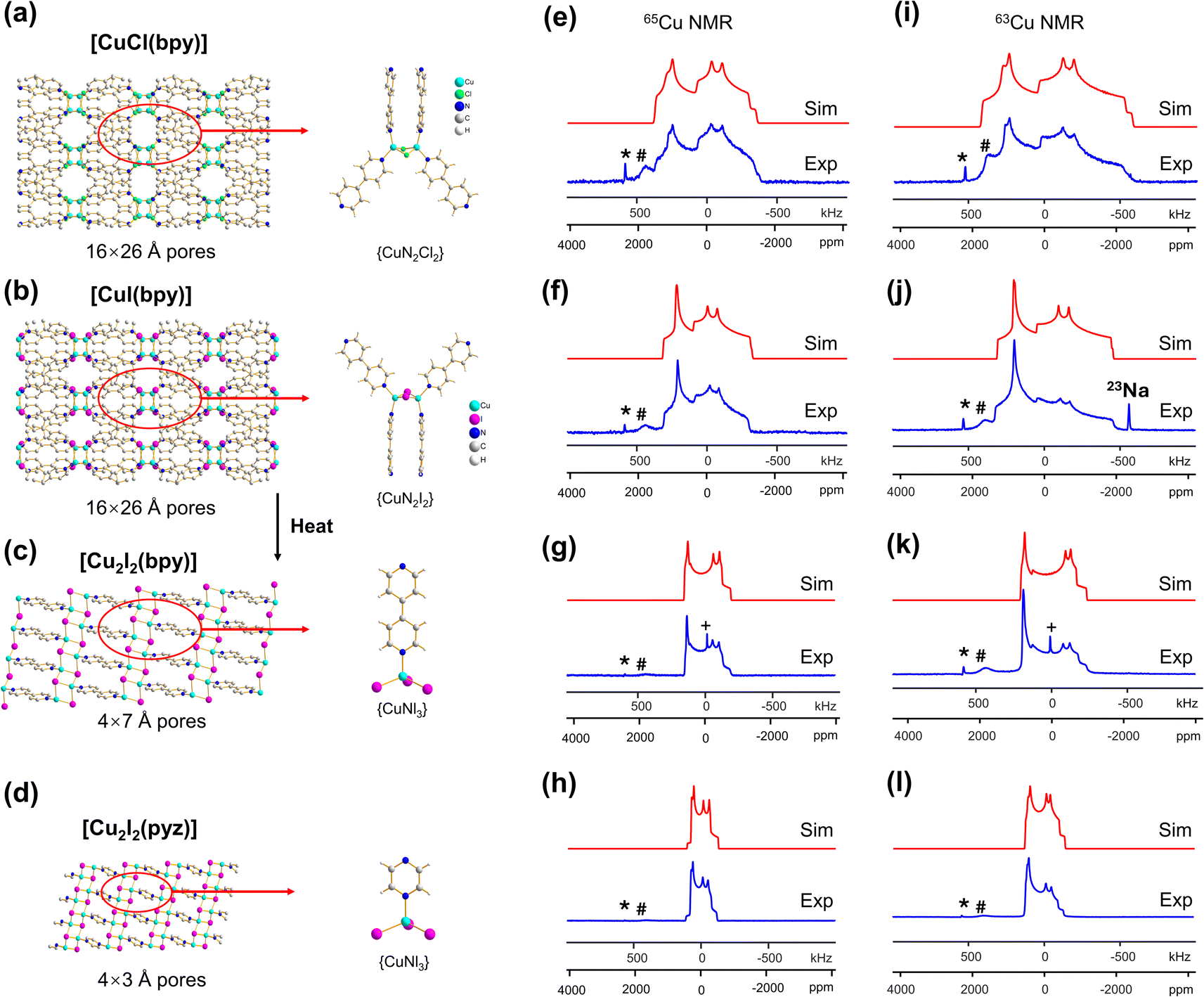 | ||
| Fig. 1 (a–d) A schematic illustration of the local and long-range structure in [CuCl(bpy)], [CuI(bpy)], [Cu2I2(bpy)], and [Cu2I2(pyz)]. The MOF pore size is listed below each structure. In (e–h), the experimental (“Exp.,” blue) and simulated (“Sim.,” red) 65Cu static NMR spectra of [CuCl(bpy)], [CuI(bpy)], [Cu2I2(bpy)] and [Cu2I2(pyz)] at 21.1 T are shown, with the corresponding 63Cu NMR spectra and simulations in (i–l). The asterisk (*) denotes a signal from metallic copper (Cu0) and the pound (#) marks a signal from probe background. The plus symbol (+) marks a resonance arising from residual CuI at 0 ppm after thermal treatment. A background 23Na signal is also noted in (j). The definitions of *, #, and + also apply to all other figures in this work. | ||
| Site | Methodb,c | C Q(65Cu)d (MHz) | C Q(63Cu)d (MHz) | η Q | δ iso (ppm) | Ω (ppm) | κ | α (°) | β (°) | γ (°) |
|---|---|---|---|---|---|---|---|---|---|---|
| a Differences between the experimental and calculated values for both the CS tensor parameters and Euler angles are considerable due to the computational difficulties involved with calculating Cu CS tensor parameters. b The “Exp.” label denotes experimental Cu NMR parameters obtained from best-fit simulations of 65/63Cu NMR spectra acquired at 21.1 T. c The “Calc.” label denotes the NMR parameters obtained from plane-wave DFT calculations using the CASTEP software package. A geometry optimization of all atoms in the reported crystal structure was performed before calculation of NMR parameters; see the Materials and Methods section for additional details. Please see Table S5 for additional calculations performed using defined cluster models. d The 65/63Cu NMR spectra were simulated independently. The experimental CQ(63Cu)/CQ(65Cu) ratio of 1.080 was found to be very close to the accepted quadrupole moment ratio Q(63Cu)/Q(65Cu) of 1.078,57 which gives additional confidence to the simulated fits. | ||||||||||
| [CuCl(bpy)] | ||||||||||
| Cu1 | Exp. | 30.0(4) | 33.5(4) | 0.45(3) | 500(50) | 600(200) | 0.4(1) | 10(3) | 28(3) | 35(3) |
| Cu1 | Calc. | 34.1 | 36.8 | 0.41 | 2188.7 | 2402.7 | −0.24 | 27.3 | 60.4 | −134.0 |
![[thin space (1/6-em)]](https://www.rsc.org/images/entities/char_2009.gif) |
||||||||||
| [CuI(bpy)] | ||||||||||
| Cu1 | Exp. | 28.7(3) | 30.2(4) | 0.50(4) | 400(50) | 300(200) | 1.0(1) | 90(2) | 35(2) | 10(2) |
| Cu1 | Calc. | 28.6 | 30.8 | 0.45 | 1215.0 | 806.2 | −0.24 | 34.3 | 45.0 | −172.4 |
|
||||||||||
| [Cu 2 I 2 (bpy)] | ||||||||||
| Cu1 | Exp. | 24.0(4) | 26.0(5) | 0.18(3) | 280(50) | 400(200) | −1.0(3) | 0(3) | 25(2) | 65(5) |
| Cu1 | Calc. | 25.5 | 27.5 | 0.47 | 867.3 | 741.4 | 0.15 | 23.4 | 20.0 | −57.2 |
|
||||||||||
| [Cu 2 Cl 2 (bpy)] | ||||||||||
| Cu1 | Exp. | 30.0(3) | 32.0(5) | 0.25(2) | 230(30) | 500(100) | 0.1(2) | 0(2) | 25(3) | 58(2) |
| Cu1 | Calc. | 27.6 | 29.4 | 0.80 | 1070.0 | 906.5 | −0.67 | 103.1 | 89.5 | 92.8 |
|
||||||||||
| [Cu 2 I 2 (pyz)] | ||||||||||
| Cu1 | Exp. | 18.8(4) | 19.6(5) | 0.35(2) | 300(50) | 480(50) | −0.8(2) | 10(3) | 25(2) | 60(4) |
| Cu1 | Calc. | 18.2 | 19.6 | 0.53 | 3701.7 | 2585.8 | −0.53 | −53.5 | 4.6 | 43.5 |
|
||||||||||
| [Cu 4 I 4 (DABCO) 2 ] | ||||||||||
| Cu1 | Exp. | 22.1(5) | 23.8(3) | 0.09(3) | 320(40) | 250(75) | 1.0(4) | 0 | 0 | 0 |
| Cu1 | Calc. | 16.4 | 17.7 | 0.22 | −58.33 | 335.57 | −0.56 | −90 | 12.5 | −180 |
| Cu2 | Exp. | 20.6(3) | 22.0(4) | 0.14(4) | 280(20) | 280(50) | 1.0(3) | 0 | 0 | 0 |
| Cu2 | Calc. | 15.3 | 16.5 | 0.37 | −90.4 | 589.8 | 0.17 | 7.4 | 85.8 | −160.5 |
| Cu3 | Exp. | 26.7(6) | 29.1(5) | 0.03(3) | 320(40) | 200(50) | 1.0(3) | 0 | 0 | 0 |
| Cu3 | Calc. | 23.0 | 24.8 | 0.02 | −58.8 | 265.7 | −0.87 | 90.0 | 5.4 | −90.0 |
|
||||||||||
| {[CuI][Cu(pdc)(H 2 O)]·1.5MeCN·H 2 O} n | ||||||||||
| Cu1 | Exp. | 22.0(3) | 24.0(2) | 0.02(2) | 400(15) | 150(200) | 1.0(4) | 0 | 0 | 0 |
| Cu1 | Calc. | 23.2 | 25.0 | 0.02 | 970.0 | 441.2 | −0.87 | 0 | 15.9 | 90 |
|
||||||||||
| Cu 2 BDC | ||||||||||
| Cu1 | Exp. | 53.0(3) | 57.0(4) | 0.22(3) | 200(150) | 1800(300) | 1.0(4) | 0 | 0 | 0 |
| Cu1 | Calc. | 57.5 | 62.0 | 0.17 | 3713.6 | 6569.0 | 0.24 | 158.7 | 2.2 | 25.4 |
|
||||||||||
| Cu(bpy) 1.5 NO 3 ·1.25H 2 O | ||||||||||
| Cu1 | Exp. | 74.0(4) | 79.0(6) | 0.18(2) | 300(100) | 0 | 0 | 0 | 0 | 0 |
| Cu1 | Calc. | 74.5 | 80.3 | 0.17 | 1337.3 | 2229.1 | 0.16 | −40.8 | 1.3 | 39.0 |
| Cu2 | Exp. | 55.2(8) | 58.5(4) | 0.00(0) | 1300(200) | 0 | 0 | 0 | 0 | 0 |
| Cu3 | Exp. | 0 | 0 | 0 | 700(100) | 0 | 0 | 0 | 0 | 0 |
|
||||||||||
| Cu 3 (4hypymca) 3 | ||||||||||
| Cu1 | Exp. | 74.8(6) | 80.6(4) | 0.55(2) | 150(200) | 0 | 0 | 0 | 0 | 0 |
| Cu1 | Calc. | 95.6 | 103.1 | 0.11 | 786.4 | 744.3 | 0.16 | 98.5 | 180.0 | −136.0 |
|
||||||||||
| SLUG-22 | ||||||||||
| Cu1,2 | Exp. | 63.0(1.0) | 67.0(8) | 0.34(2) | 100(150) | 1500(200) | 1.0(1) | 0 | 0 | 0 |
| Cu1 | Calc. | 40.0 | 44.2 | 0.74 | 786.5 | 3181.5 | −0.24 | 174.4 | 172.4 | 53.0 |
| Cu2 | Calc. | 42.2 | 45.5 | 0.86 | 859.8 | 3055.1 | −0.24 | −17.3 | 3.17 | −22.3 |
|
||||||||||
| [Cu 6 I 6 (DABCO) 2 ] | ||||||||||
| Cu1,2,3 | Exp. | 19.1(3) | 21.4(3) | 0.70(2) | 670(20) | 0 | 0 | 0 | 0 | 0 |
| Cu1 | Calc. | 19.2 | 20.7 | 0.54 | 81.27 | 709.4 | 0.45 | −28.6 | 125.2 | 175.7 |
| Cu2 | Calc. | 19.3 | 20.8 | 0.25 | 124.5 | 724.9 | −0.18 | 96.3 | 21.1 | −143.4 |
| Cu3 | Calc. | 7.2 | 7.8 | 0.34 | 324.5 | 704.7 | 0.53 | 0 | 104.3 | 0 |
| Cu4 | Exp. | 24.1(2) | 27.0(2) | 0.20(3) | 280(50) | 0 | 0 | 0 | 0 | 0 |
| Cu4 | Calc. | 24.1 | 26.0 | 0.24 | 257.0 | 868.6 | −0.90 | −90 | 0.22 | 90 |
|
||||||||||
| Cu 2 (pyz) 2 (SO 4 )(H 2 O) 2 | ||||||||||
| Cu1 | Exp. | 25.2(2) | 27.2(4) | 0.54(2) | 500(100) | 900(100) | 0.0 | 70(2) | −4(2) | −11(3) |
| Cu1 | Calc. | 23.7 | 25.5 | 0.55 | 2079.4 | 2995 | −0.39 | 43.5 | 58.0 | −73.0 |
The [CuI(bpy)] MOF (Fig. 1(b)) has a topology and local coordination of Cu(I) ions similar to that in [CuCl(bpy)]. The main difference between these compounds is that the Cu–I bond length in [CuI(bpy)] is ca. 0.2 Å longer than the Cu–Cl distance in [CuCl(bpy)]. The Cu NMR powder pattern (Fig. 1(f and j)) could be simulated using one unique Cu site (Table 1). [CuI(bpy)] has a lower CQ and slightly higher ηQ (CQ(65Cu) = 28.7(3) MHz, ηQ = 0.50(4)) than [CuCl(bpy)], partially due to the more ionic nature of the Cu–I bond, illustrating the sensitivity of Cu NMR to local structure.
The three-dimensional porous [CuI(bpy)] MOF is transformed to two-dimensional [Cu2I2(bpy)] with heat (Fig. 1(b, c) and S4†).65 [CuI(bpy)] crystallizes in the I41/acd space group. The single unique Cu(I) center resides in a CuN2I2 slightly distorted tetrahedral local environment, which involves bonding to two N atoms from separate 4,4′-bpy ligands along with two bridging μ2-I ligands. In contrast, [Cu2I2(bpy)] is a two-dimensional layered material that crystallizes in the P![[1 with combining macron]](https://www.rsc.org/images/entities/char_0031_0304.gif) space group with layer stacking along the crystallographic b axis. In [Cu2I2(bpy)], there is one Cu(I) site in a CuNI3 distorted tetrahedral environment, which is bound to three μ3-I species and one nitrogen atom from the 4,4′-bpy ligands. 63/65Cu solid-state NMR experiments were performed to investigate the local structure at Cu in both [CuI(bpy)] and the [Cu2I2(bpy)] product from thermal treatment (Fig. 1(b and c)). These MOFs give rise to well-defined 63/65Cu NMR powder patterns, which are dominated by the QI but also influenced by CSA, and are both indicative of one unique Cu site. The NMR spectra of [CuI(bpy)] and [Cu2I2(bpy)] are visually distinct and yield different 63/65Cu NMR parameters (Table 1). The CQ(65Cu) value of 28.7(3) MHz in [CuI(bpy)] is reduced to 24.0(4) MHz in [Cu2I2(bpy)], with the increased symmetry at Cu attributed to the change from a CuN2I2 to a CuNI3 local environment. The ηQ parameter is also sensitive to the phase change, falling from 0.50(4) in [CuI(bpy)] to 0.18(3) in [Cu2I2(bpy)], which is indicative of increased axial symmetry about the Cu center in [Cu2I2(bpy)].
space group with layer stacking along the crystallographic b axis. In [Cu2I2(bpy)], there is one Cu(I) site in a CuNI3 distorted tetrahedral environment, which is bound to three μ3-I species and one nitrogen atom from the 4,4′-bpy ligands. 63/65Cu solid-state NMR experiments were performed to investigate the local structure at Cu in both [CuI(bpy)] and the [Cu2I2(bpy)] product from thermal treatment (Fig. 1(b and c)). These MOFs give rise to well-defined 63/65Cu NMR powder patterns, which are dominated by the QI but also influenced by CSA, and are both indicative of one unique Cu site. The NMR spectra of [CuI(bpy)] and [Cu2I2(bpy)] are visually distinct and yield different 63/65Cu NMR parameters (Table 1). The CQ(65Cu) value of 28.7(3) MHz in [CuI(bpy)] is reduced to 24.0(4) MHz in [Cu2I2(bpy)], with the increased symmetry at Cu attributed to the change from a CuN2I2 to a CuNI3 local environment. The ηQ parameter is also sensitive to the phase change, falling from 0.50(4) in [CuI(bpy)] to 0.18(3) in [Cu2I2(bpy)], which is indicative of increased axial symmetry about the Cu center in [Cu2I2(bpy)].
In a manner similar to [CuI(bpy)], the three-dimensional [CuCl(bpy)] MOF can also undergo a transformation to the two-dimensional [Cu2Cl2(bpy)] MOF upon thermal treatment. The 63/65Cu NMR spectra of these two MOFs (Fig. S5†) are distinct and diagnostic of the phase change. While the CQ(Cu) values are very similar in both forms, ηQ changes from 0.45(3) in [CuCl(bpy)] to 0.25(2) in [Cu2Cl2(bpy)] (Table 1), producing a clear spectral difference indicative of a significant increase in local axial symmetry. The results indicate that 63/65Cu NMR is a viable spectroscopic route for tracking phase changes in Cu MOFs.
) and has one unique Cu(I) site residing in a distorted tetrahedral CuNI3 environment. While the Cu(I) local bonding geometries are similar between [Cu2I2(bpy)] and [Cu2I2(pyz)],65,67 the 63/65Cu NMR powder patterns are relatively narrower in [Cu2I2(pyz)] (Fig. 1), and CQ(65Cu) falls from 24.0(4) MHz in [Cu2I2(bpy)] to 18.8(4) MHz in [Cu2I2(pyz)]. One reason for the decrease in CQ is the smaller bond angle and bond length distributions involving Cu, while another possibility lies in long-range influences on the EFG that originate beyond the first coordination sphere of Cu (i.e., the effect of different N-bound linker groups). A more detailed discussion can be found in the ESI.†
Many MOFs containing CuxIy clusters feature multiple unique Cu(I) sites and have luminescent properties. The luminescent [Cu4I4(DABCO)2] MOF is composed of Cu4I4 clusters along with 1,4-diazabicyclo[2.2.2]octane (DABCO) linkers (Fig. 2(a)).12 This material crystallizes in the P4/mcc space group and has three inequivalent Cu(I) sites in the Cu4I4 unit, where the Cu sites are populated in the ratio Cu1:Cu2:Cu3 = 1:2:1. Each inequivalent Cu(I) site resides in a CuNI3 distorted tetrahedral environment, with the three coordinated iodine atoms originating from the Cu4I4 cluster and the nitrogen atom from a DABCO linker. The 63/65Cu NMR spectra (Fig. 2(b and c)) are both >400 kHz broad at 21.1 T, with fine features that hint at overlapping Cu resonances. Simulations of experimental data confirm that there are two narrower and overlapping Cu signals of higher intensity nested within a less intense, broader underlying signal; the NMR parameters obtained from simulations are summarized in Table 1.
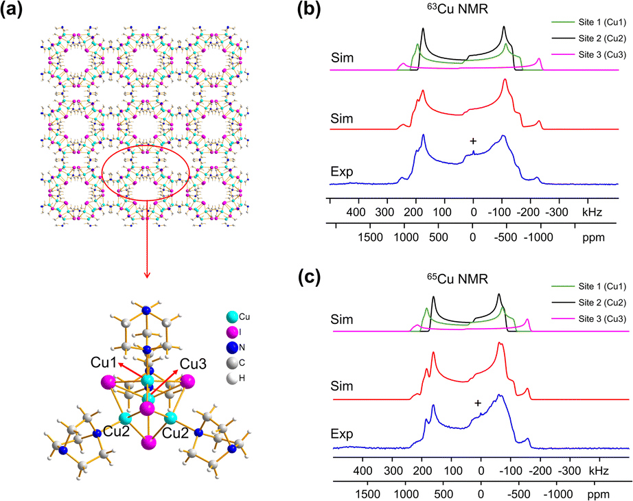 | ||
| Fig. 2 A schematic illustration of the long-range structure of [Cu4I4(DABCO)2] along with the local structure about Cu is shown in (a). The experimental (b) 63Cu and (c) 65Cu static NMR spectra (blue), cumulative simulations (red), and individual Cu site simulations (black, purple, green) of [Cu4I4(DABCO)2] at 21.1 T are also included. | ||
With the NMR parameters successfully extracted, plane-wave DFT calculations were performed to assign 63/65Cu resonances to crystallographic sites. The calculated 63/65Cu NMR parameters (Table 1) indicate that Cu sites 1 and 2 should exhibit similar NMR parameters, including relatively smaller CQ(63/65Cu) values, while site 3 should correspond to unique NMR parameters and a larger CQ(63/65Cu). Accordingly, the two narrower components of the spectrum were assigned to Cu sites 1 and 2, with the broader signal corresponding to site 3. Given the similarities in CQ values between Cu sites 1 and 2, an alternate NMR parameter, such as ηQ, must be used to distinguish between them. A careful examination of the left quadrupolar “horn” of the two narrower signals located between +150 and +250 kHz in the 63Cu NMR spectra reveals significant detail, which differentiates the Cu1 and Cu2 powder patterns based on ηQ values. A comparison of local structural parameters between Cu2 and Cu1 shows that Cu2 has both the larger Cu–I bond length distribution and ∠N–Cu–I distribution of all Cu sites;12 this combination reflects a relatively lower axial symmetry in the Cu2 local environment and should result in a relatively higher ηQ value. Cu2 is thus assigned to the signal with ηQ = 0.14(4) and Cu1 is assigned to the signal with a smaller ηQ of 0.09(3). This assignment is also consistent with DFT calculations (Table 1, where ηQ(Cu2) > ηQ(Cu1) > ηQ(Cu3)). For a more detailed discussion, please see the ESI.†
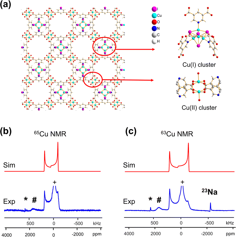 | ||
| Fig. 3 (a) A schematic illustration of the long-range and local structure in the {[Cu(I)][Cu(II)(pdc)(H2O)]·1.5MeCN·H2O}n MOF, including the Cu(I) and Cu(II) clusters. The blue experimental and red simulated (b) 65Cu and (c) 63Cu static NMR spectra at 21.1 T are also shown. | ||
A CQ(65Cu) value of 22.0(3) MHz and ηQ of 0.02(2) were obtained from {[Cu(I)][Cu(II)(pdc)(H2O)]·1.5MeCN·H2O}n; the near-zero ηQ value is in good agreement with the high local rotational symmetry at Cu(I) indicated from the single crystal XRD structure.72 The very slight departure from perfect C3 rotational symmetry indicated by the ηQ value of 0.02 can be traced to one of the Cu-bonded iodine atoms, which lies slightly out of a truly C3 symmetrical ligand arrangement. The dominance of the QI on 63/65Cu NMR spectral appearance, paired with the high signal-to-noise ratio, indicates that there is very little paramagnetic influence on the Cu(I) NMR parameters. The lack of paramagnetic effects can be attributed to two reasons. First, the paddlewheel Cu2 dimer in its ground state is an antiferromagnetically coupled spin singlet due to the short Cu–Cu bond length;73 the EPR spectrum of this MOF yielded a g-value of 2.161 (Fig. S7(b)†), which falls in the range of reported g-values for MOFs containing a Cu2 dimer in paddle-wheel units.74–78 Second, the distance between the Cu(I) and Cu(II) dimers is 7.05 Å, which is long enough that the Cu(I) spin energy levels are only perturbed to a minor degree by any paramagnetic interaction.
In addition to the direct synthesis of Cu (I/II) MOFs, a post-synthetic approach to Cu(I/II) MOFs affords alternate avenues for tuning MOF properties; however, it is difficult or impossible to obtain diffraction-caliber single crystals of product using this approach. Potential applications for 63/65Cu solid-state NMR in the characterization of post-reduction Cu(I)-containing MOFs were explored by examining the case of Cu2BDC synthesis from the reduction of CuBDC. Cu(II) sites in the two-dimensional CuBDC (BDC, 1,4-benzendicarboxylic acid) MOF can be partially reduced with L-ascorbic acid (LA acid) via post-synthetic modification to introduce Cu(I) sites, forming a three-dimensional Cu2BDC MOF (Fig. 4(a)).14 Powder XRD (Fig. S9†) clearly indicates that Cu2BDC resides in a different phase than the parent CuBDC MOF, but further analysis of the Cu local environment is hampered by the difficulties in obtaining Cu2BDC single crystals. The parent CuBDC MOF contains a paddlewheel local structure about Cu, where each Cu(II) center is linked to four carboxylic groups from BDC linkers along with one water molecule, forming a stacked layered structure held together through intermolecular interactions. After LA-acid post-synthetic modification to produce the Cu2BDC MOF, half of the Cu(II) sites in the MOF were reduced to Cu(I) (Fig. 4(a)). The four-coordinate Cu(I) center in Cu2BDC resides in a local CuO4 environment of seesaw geometry, with Cu(I) connected to two carboxylic oxygen atoms (O1, O2) from two BDC ligands, one oxygen atom (O3) of a water molecule, and one oxygen atom (O4) of a bridging OH group. The successful reduction of Cu(II) centers to Cu(I) was confirmed by Cu 2p3/2 X-ray photoelectron spectroscopy (XPS, Fig. S9†) and X-band EPR (Fig. S10†). The 63/65Cu NMR spectra of Cu2BDC (Fig. 4(b and c)) features a QI-dominated NMR powder pattern that yields CQ(65Cu) = 53.0(3) MHz and ηQ = 0.22(3); the well-defined spectrum with relatively sharp features is also indicative of a highly ordered local structure. Although Cu(I) is four-coordinate in this system, the CQ value is much larger than those of other four-coordinate Cu(I) centers previously discussed. This discrepancy arises from the seesaw local geometry about Cu(I) in Cu2BDC, which is a much more significant deviation from tetrahedral symmetry versus previous examples of distorted tetrahedral geometry.
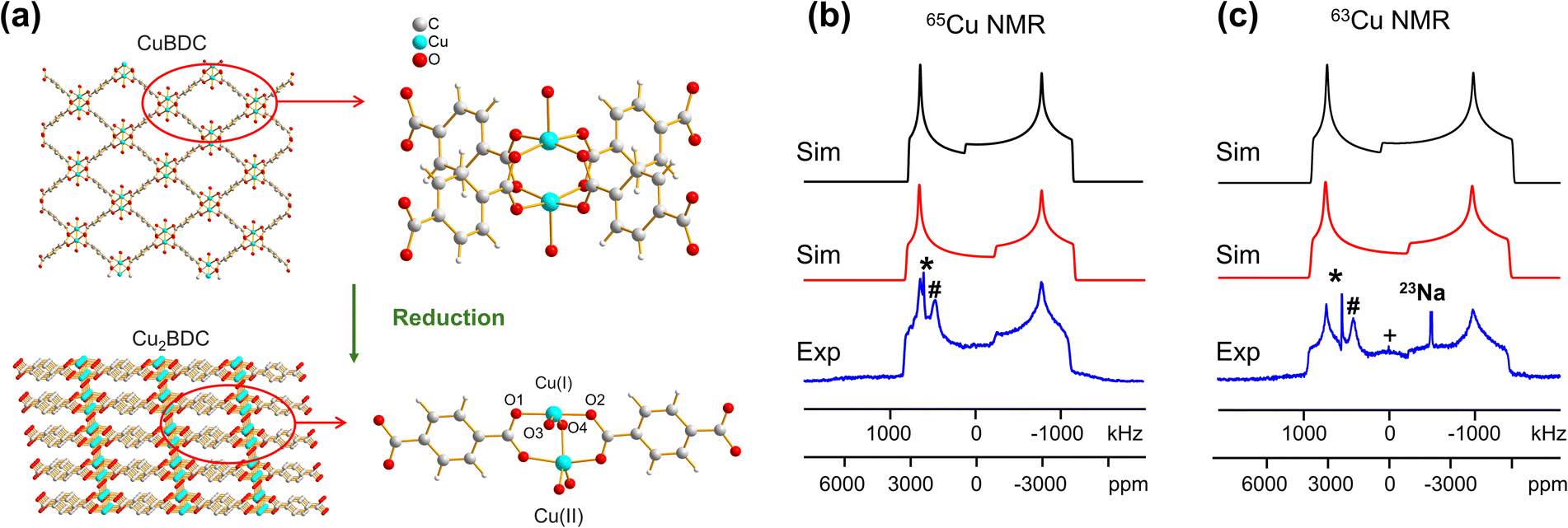 | ||
| Fig. 4 (a) The reduction of CuBDC to Cu2BDC and the local environment of Cu(I) in CuBDC and Cu2BDC is pictured. (b) Blue experimental (b) 65Cu and (c) 63Cu static NMR spectra of Cu2BDC at 21.1 T are shown, along with simulations incorporating CSA effects (red trace) and neglecting CSA effects (black trace). Note the effects of CSA on the central spectral discontinuity. The signal from 23Na background is also indicated in the 63Cu NMR spectrum but truncated for clarity. | ||
A CSA span value of 1800 ppm was necessary to achieve good agreement between the simulated and experimental 63/65Cu NMR spectra of Cu2BDC (Fig. 4(b and c)), owing to the hyperfine interaction. The presence of paramagnetic centers, with their associated unpaired electrons, influences the NMR spectral appearance and CSA parameters of nearby diamagnetic nuclei.79–83 The corresponding hyperfine interactions between Cu(II) unpaired electrons and Cu(I) nuclei leads to very large 63/65Cu NMR span values. We have performed localized molecular orbital calculations on Cu2BDC, which revealed that the unpaired electrons of Cu(II) are indeed able to sample regions proximate to Cu(I) (Fig. S11†); this finding, together with the unremarkable Cu chemical shift of 200 ppm, indicates that an electron delocalization effect is present rather than a spin-polarization effect.79,82,83 This shows how 63/65Cu NMR can be a robust local characterization technique in the presence of proximate paramagnetic Cu(II) centers, extending the applications of this technique to a wider variety of Cu MOFs.
MOFs with three-coordinate Cu(I) sites
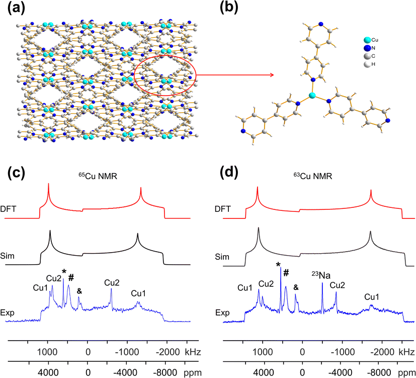 | ||
| Fig. 5 (a) The 3D framework structure and (b) local structure of the Cu(bpy)1.5NO3·1.25H2O MOF. The charge-balancing NO3− anion and guest water molecules are omitted for clarity. (c) 65Cu and (d) 63Cu static NMR spectra of Cu(bpy)1.5NO3·1.25H2O at 21.1 T; the blue traces are experimental, black are simulated, and red are simulated using NMR parameters from DFT calculations. | ||
The 63/65Cu static solid-state NMR spectra of the as-made hydrated Cu(bpy)1.5NO3·1.25H2O MOF at 21.1 T are shown in Fig. 5(c and d). The local Cu environment is significantly distorted from trigonal planar symmetry (∠N1–Cu–N2 = 125.39°, ∠N1–Cu–N3 = 125.71°, ∠N2–Cu–N3 = 108.54°), which leads to an increased CQ(63/65Cu) value and spreads the 63/65Cu NMR spectral powder patterns across breadths of ca. 3 MHz and 4 MHz, respectively. The 63/65Cu NMR spectra feature a broad signal with some additional details, along with metallic copper (*) and background signals (#).
A successful simulation of all spectral features is challenging due to the multiple Cu powder patterns, despite the single Cu(I) site present in this MOF. Several spectral simulation strategies were explored, but only one produced a satisfactory fit (Fig. S12†), which is discussed below. The extremely broad underlying powder pattern with corresponding quadrupolar horns marked “Cu1” in Fig. 5, which has the highest integrated ratio of ca. 80%, originates from the Cu(bpy)1.5NO3·1.25H2O MOF. The extracted parameters are CQ(65Cu) = 74.0(4) MHz, CQ(63Cu) = 79.0(6) MHz, ηQ = 0.18(2), and δiso = 300(100) ppm, where both CQ values are remarkably high among reported values.35,51 This assignment is also supported by DFT calculations, which yielded CQ,calc (65Cu) = 74.5 MHz and ηQ,calc = 0.17 (Table 1, Fig. 5(c and d)). Another narrower resonance labelled Cu2, with an integrated area ratio of ca. 18%, is assigned to a side product; the NMR parameters are reported in Table 1 for reference. The experimental PXRD pattern of Cu(bpy)1.5NO3·1.25H2O in Fig. S2† agrees well with the pattern simulated from the reported crystal structure, yet the experimental diffractogram also exhibits some additional reflections at low angles that are attributed to the Cu(I) impurity. There is also a trace amount of an unidentified impurity accounting for ca. 2% of total spectral intensity that is labelled with the “&” character and assigned to a Cu3 species.
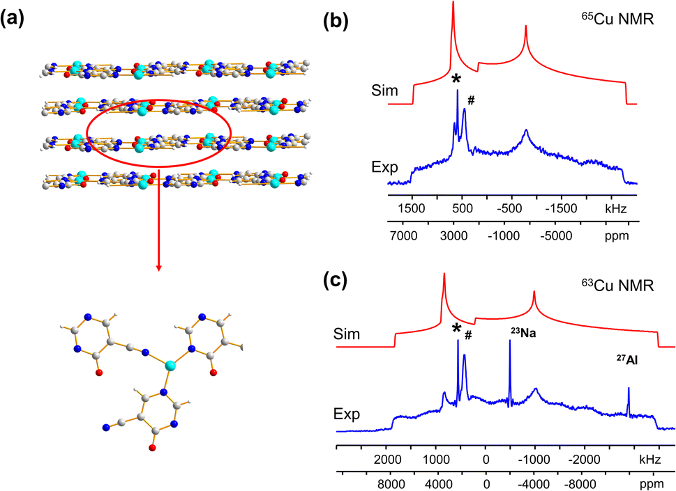 | ||
| Fig. 6 (a) The long-range and local structure of Cu3(4hypymca)3. The experimental (blue) and simulated (red) 65Cu static NMR spectra and 63Cu static NMR spectra at 21.1 T are shown in (b and c), respectively. 27Al marks a signal from probe background. The signal from 23Na background is also marked in the 63Cu NMR spectrum, but is truncated for clarity. | ||
While both [Cu3(4hypymca)3] and Cu(bpy)1.5NO3·1.25H2O feature Cu(I) bound to three nitrogen atoms, the ηQ value is significantly higher in [Cu3(4hypymca)3] (Table 1). Cu(bpy)1.5NO3·1.25H2O features Cu coordinated to three N atoms of pyridine groups, but the Cu center in [Cu3(4hypymca)3] is connected to two pyridine-based N atoms and one nitrile N atom, which corresponds to decreased axial symmetry about Cu and a higher ηQ value. The average trigonal distortion ( , where θi, i = 1, 2, 3 are the three ∠N–Cu–N bond angles around Cu) is also larger in [Cu3(4hypymca)3] than in Cu(bpy)1.5NO3·1.25H2O by 8.0°, which further explains the increase in ηQ.
MOFs with two-coordinate Cu(I) sites
Some MOFs feature Cu(I) in two-coordinate linear arrangements. The SLUG-22 MOF is composed of Cu2(4,4′-bpy)2 units, where the two-coordinate Cu(I) center is connected to two nitrogen atoms from separate 4,4′-bpy linkers in a distorted N–Cu–N linear geometry, with a long-range structure consisting of one-dimensional chains of infinite length (Fig. 7(a)). 63/65Cu static solid-state NMR spectra of SLUG-22 at 21.1 T (Fig. 7(b and c)) are extremely broad, owing to the low local symmetry of the linear two-coordinate environment at Cu and the correspondingly large CQ value. Simulations (Table 1) necessitated the use of CS parameters, but indicated only a single Cu(I) site with CQ(65Cu) = 63.0(1.0) MHz and ηQ = 0.34(2) was present; this contrasts with the reported crystal structure18 that indicated there are two inequivalent Cu(I) sites. A careful examination of the 63/65Cu NMR spectra reveals slightly broader features in the experimental spectra, which could be indicative of two nearly identical overlapping Cu powder patterns that cannot be resolved. Indeed, the crystal structure shows that the Cu centers reside in very similar local environments.18 Furthermore, Fig. 7 illustrates how the frequency of the central spectral discontinuity is affected by CSA, and in particular, the exceptionally large span value of 1500 ppm.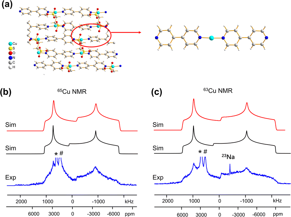 | ||
| Fig. 7 (a) The 3D framework structure and local structure of the SLUG-22 MOF. The (b) 65Cu and (c) 63Cu static NMR spectra at 21.1 T are shown in blue, along with the red simulation which includes CSA effects, and the black trace which does not include CSA effects. Note the difference in the central “divot” spectral feature between the red (CSA) and black (no CSA) simulations; CSA is necessary to properly fit this feature. The asterisks (*) denote the signal from metallic copper (Cu0) and the pound (#) marks the signal from probe background, which are truncated for clarity. The signal from 23Na background is also marked in the 63Cu NMR spectrum. | ||
In order to investigate the origins of the abnormally large Cu CSA in SLUG-22, EPR and XPS experiments were performed (Fig. S13†), which indicated this material was largely free of Cu(II) or other paramagnetic impurities. The lack of any plausible hyperfine interactions indicates the sizeable CSA in SLUG-22 likely arises from the linear two-coordinate local geometry at Cu. Large CSA spans have been recorded from other transition metal compounds in linear configurations (e.g., linear HgX2).85 We found that cluster DFT calculations using the RHF method and 6-31++G**/6-311++G** basis sets were the most reliable avenue for calculating Cu span values (vide infra, Table S5†); these particular calculations also predicted a substantial Cu CSA span value in SLUG-22 arising from the local linear coordination geometry at Cu.
There are more complicated MOFs featuring mixed coordinate Cu(I) local environments that can be examined using 63/65Cu NMR. We investigated the [Cu6I6(DABCO)2] framework, which contains four distinct Cu sites and produced a complicated Cu NMR spectrum that lacked clear singularities. The results and discussion regarding these experiments can be found in the ESI.†
DFT calculations of EFG tensors
To obtain further insight into experimental NMR results and the local Cu(I) environments, plane-wave DFT calculations using GIPAW methods were performed. The EFG tensor parameters are sensitive to the local environment, which provides a metric to predict and optimize crystal structures.86–92 In this section, we examine Cu(I) structural insights obtained from plane-wave DFT calculations of 63/65Cu EFG tensors in MOFs. It should be noted that the XRD crystal structures were obtained at low temperatures while our Cu NMR experiments were performed at room temperature, which could lead to discrepancies between calculated and experimental Cu NMR parameters due to issues such as temperature-dependent unit cell dimensions and dynamics. To verify that temperature changes did not introduce significant changes to Cu NMR parameters, low-temperature NMR experiments were performed on selected MOFs, which yielded Cu NMR spectra nearly identical to room temperature spectra (Fig. S15†). This finding signified that, in this case, the experimental temperature did not play a significant role in the accuracy of calculated NMR parameters. This result is not particularly surprising, as all the MOFs investigated in this work have rather rigid frameworks.GIPAW DFT calculations on the Cu MOF systems were evaluated by first examining the correlations between the calculated and experimental EFG tensor parameters in discrete Cu(I) coordination complexes with relevant Cu(I) local environments. The experimental Cu NMR data was taken from previous reports by Tang35 and Yu,56 using crystal structures obtained from the Cambridge Crystallographic Data Centre (CCDC). As shown in Fig. S16 and Appendix A of the ESI,† the calculated principal components of the Cu EFG tensor in this dataset exhibit a decreased ΓRMSE (the EFG distance metric expressing the deviation between experimental and computed EFG parameters;93 see ESI†) after geometry optimization, from 0.071 a.u. before to 0.053 a.u. after. After geometry optimization, the slope of the respective plot is closer to 1, the y-intercept is reduced, and R2 is higher, which all indicate a better agreement with experimental values.
The correlation between DFT-calculated and experimental Cu EFG tensor components |Vkk| (k = 1, 2, 3) based on our current MOF dataset are shown in Fig. 8(a and b). After geometry optimization, the ΓRMSE of the MOF Cu dataset was calculated to be 0.119 a.u., which is significantly larger than the 0.053 a.u. of the dataset constructed from prior reports. Bar plots of calculated versus experimental CQ and ηQ values are shown in Fig. S25;†CQ depends on a single EFG tensor component (V33) and is generally calculated quite accurately, while ηQ calculations are dependent on all three EFG tensor components and are therefore less accurate. The SLUG-22 and Cu3(4hypymca)3 MOFs are responsible for the increased Γ value in the MOF dataset (Fig. 8(c)). When excluding SLUG-22 and Cu3(4hypymca)3, the ΓRMSE value is a much more reasonable 0.047 a.u. These results indicate that further investigation of the local structure and geometry optimization in SLUG-22 and Cu3(4hypymca)3 is warranted.
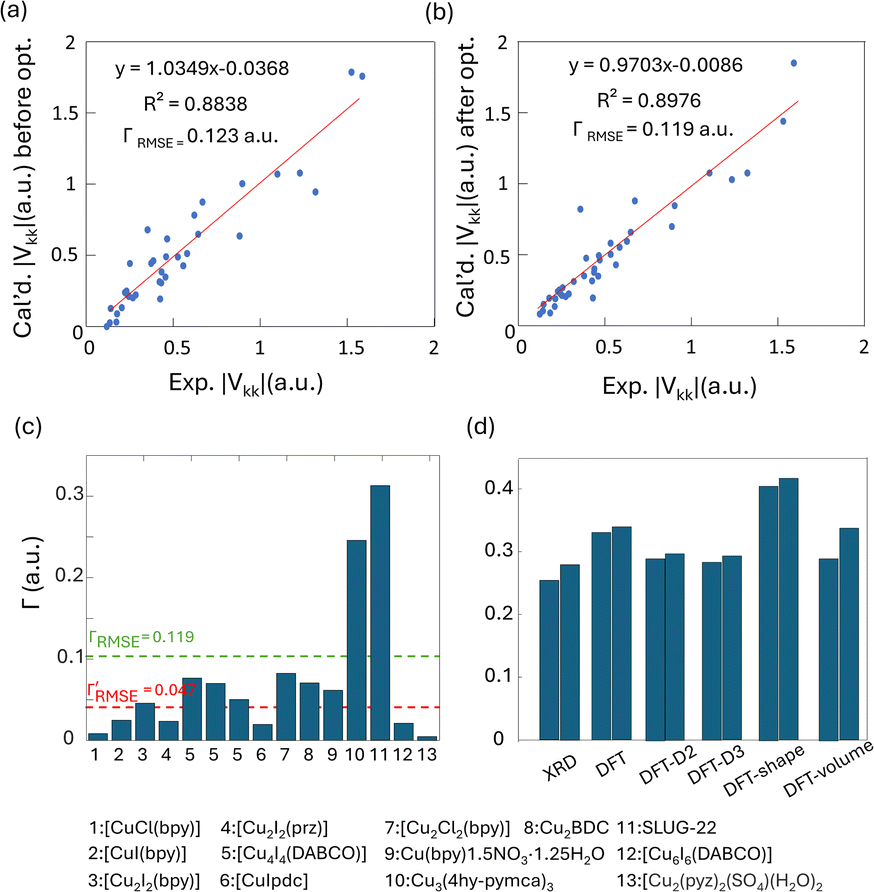 | ||
| Fig. 8 Relationships between the principal components (|Vkk|, k = 1,2,3) of calculated and experimental 63/65Cu EFG tensors in MOFs (a) before and (b) after geometry optimization. (c) The Γ values for all MOFs after geometry optimization. The ΓRMSE including the results from all MOFs is shown as a green dashed line, while the ΓRMSE excluding SLUG-22 and Cu3(4hypymca)3 is shown as a red dashed line. (d) The EFG distance in the optimized SLUG-22 structure is shown, as obtained after plane-wave DFT calculations using different geometry optimization approaches. The x-axis labels in (d) are as follows; XRD structure: no optimization; DFT: geometry optimization without optimization of unit cell dimensions; DFT-shape: optimization with unit cell using a fixed-shape constraint; DFT-volume: optimization with unit cell dimensions using a fixed-volume constraint; DFT-D2 and DFT-D3: optimization using the D2 and D3 dispersion corrections with an optimized damping parameter (Fig. S17†).86,93 Note that there are two inequivalent but similar Cu sites in the reported XRD structure of SLUG-22. | ||
Four DFT optimization schemes of the SLUG-22 crystal structure were explored (Fig. 8(d)). All the geometry-optimized structures yielded lower SCF energies versus the XRD structure, yet the agreement between calculated and experimental Cu EFG tensor parameters using any of the calculation strategies did not show significant improvement, which is puzzling. A more detailed examination of the experimental PXRD patterns in the original work describing SLUG-2218 (Fig. S19(a)†) revealed that several intense reflections expected at low angles from the reported single crystal structure are not apparent in the original experimental data, particularly the prominent reflection at ca. 9°, while additional unexpected reflections are present. Our geometry-optimized structures generated using a myriad of DFT-based approaches failed to improve the agreement between experimental and calculated XRD patterns (Fig. S19(b)†). Based on the considerable deviation between the experimental and calculated PXRD patterns, along with the inaccuracy of calculated EFG tensor parameters, it appears that the reported single crystal structure of SLUG-22 is incorrect in some manner, which illustrates another practical application of Cu NMR.
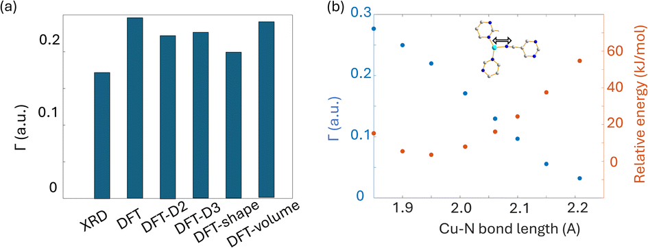 | ||
| Fig. 9 (a) The EFG distance of optimized Cu3(4hypymca)3 structure with different approaches, along with (b) the dependence of Γ on Cu–N bond length. | ||
We also performed calculations on geometry-optimized cluster models. The results using several different methods and basis sets are listed in Table S5.† The CS span values calculated using RHF/6-31++G** and RHF/6-311++G** (Fig. S21†) demonstrated better agreement with experimental span values when compared to plane-wave DFT calculations. In contrast, the calculated EFG tensors with all cluster models (Fig. S20†) yielded poorer agreement with experimental values when compared to plane-wave DFT calculations (Fig. 8(b)).
Quadrupolar coupling constant and the Cu(I) coordination number
The observed quadrupolar coupling constant (CQ) largely depends on the coordination number of Cu(I). A summary of the CQ(65Cu) values in MOFs is illustrated in Fig. 10, along with relevant values in small metal–organic coordination compounds from previous reports.35,51,56 The CQ(65Cu) values of four-coordinate tetrahedral Cu(I) centers are generally <40 MHz. The CQ(65Cu) values of three-coordinate Cu(I) range from 40 MHz to 80 MHz. Four-coordinate Cu(I) in a pseudo-three coordinate environment is correlated to CQ(65Cu) values between 40 and 50 MHz,51 which lies just between the bulk of four- and three-coordinate Cu environments. 63/65Cu NMR reports on two-coordinate Cu(I) ions are not common; both the SLUG-22 MOF in this work and the previously reported small molecule ClCuP(2,4,6)335 yielded CQ(65Cu) values between 60 and 65 MHz. There were no prior 63/65Cu solid-state NMR reports of Cu(I) centers in a four-coordinate seesaw local geometry before this work; this environment appears to produce CQ values comparable to three- and two-coordinate Cu(I) arrangements. The compiled empirical results from this and prior studies in Fig. 10 provides a convenient and general NMR-based tool to estimate the coordinate state of Cu(I) in unknown environments across a variety of materials and compounds.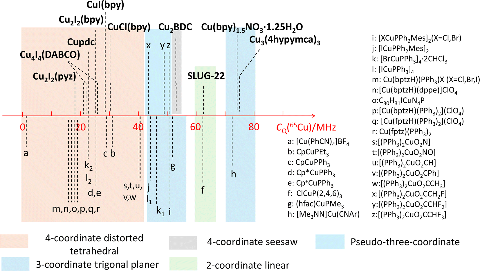 | ||
| Fig. 10 Copper CQ(65Cu) values of Cu(I) MOFs, along with those previously reported for other Cu(I) compounds. | ||
65Cu solid-state NMR at 9.4 T
The Cu MOFs in this study were examined by 63/65Cu NMR using a high magnetic field of 21.1 T. Unfortunately, high fields are not always readily accessible, but there are several previous studies regarding 65Cu ultra-wideline NMR at 9.4 T.35,51 In MOFs, the Cu concentration is diluted, which poses an additional obstacle.We set out to find if 65Cu solid-state NMR of Cu(I) MOFs was feasible at a more accessible field of 9.4 T (i.e., ν0(1H) = 400 MHz), which would open up this technique to researchers across a broad swath of institutions. In addition, performing the Cu NMR experiments at different magnetic fields allows one to extract unambiguous CS and QI parameters along with the second-order quadrupolar isotropic shift. A major challenge at 9.4 T is spectral width; broadening from the second-order quadrupolar interaction is inversely proportional to B0, thus 63/65Cu NMR spectra are spread across a significantly larger frequency range at lower magnetic fields. To increase the signal-to-noise ratio and reduce experimental times, the WURST-CPMG pulse sequence can be employed.100 The WURST-CPMG sequence yields NMR spectra composed of a series of spikelets that trace out the overall spectral manifold, rather than the smooth continuous lineshape obtained from solid echo experiments. A spikelet spectrum can be acquired significantly faster than a solid echo spectrum. Using seven Cu(I) MOFs from this study as examples, we obtained 65Cu NMR spectra at 9.4 T ranging from ca. 500 to 3000 kHz in breadth (Fig. 11). The 9.4 T data was then simulated independently in order to assess the reliability of these results against those obtained at 21.1 T. The 65Cu NMR parameters obtained at 9.4 T (Table S6†) were consistent with those obtained from 63/65Cu experiments at 21.1 T, validating the accuracy of the extracted NMR parameters in Table 1. These findings prove that 63/65Cu NMR of Cu(I) MOFs and other Cu-dilute systems is experimentally viable at 9.4 T. The experimental times are listed in Table S4.†
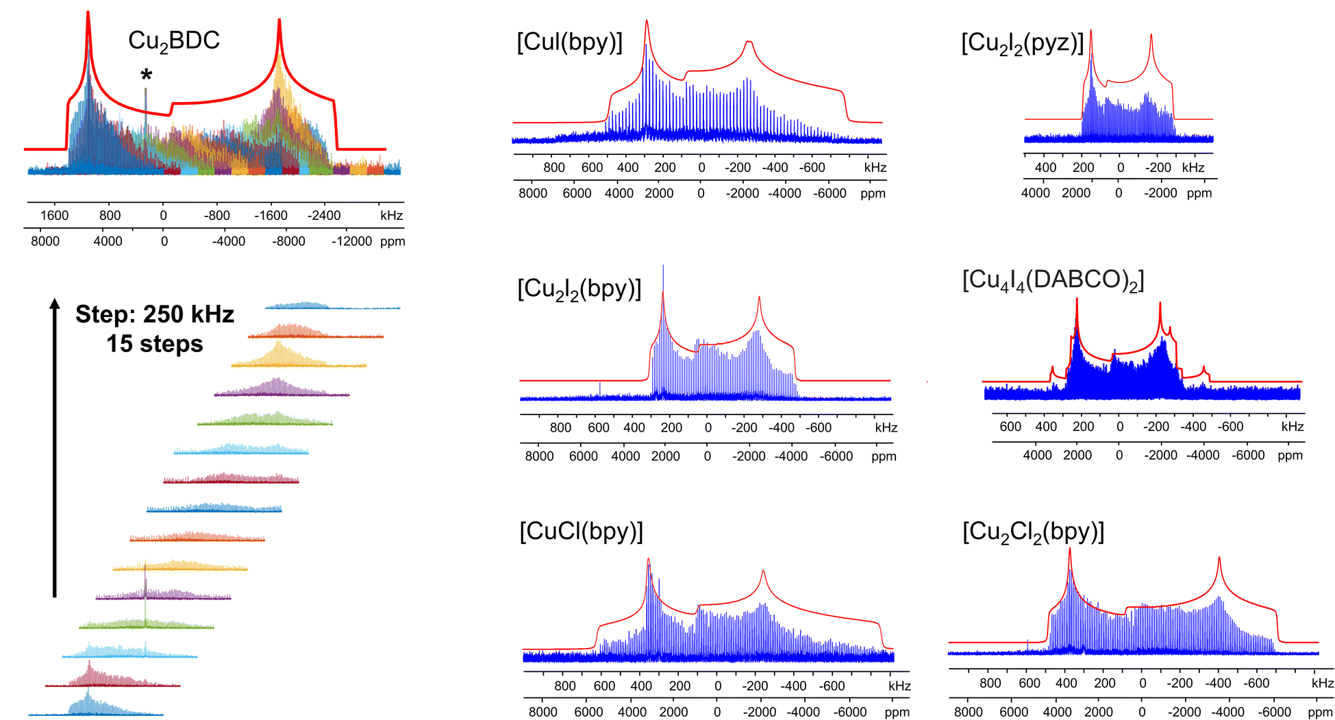 | ||
| Fig. 11 The experimental (blue) and simulated (red) 65Cu static WURST-CPMG NMR spectra of [CuCl(bpy)], [Cu2Cl2(bpy)] [CuI(bpy)], [Cu2I2(bpy)], [Cu2I2(pyz)] and [Cu4I4(DABCO)2] at 9.4 T are shown at right, along the 15 sub-spectra required to assemble the overall spectrum of Cu2BDC at left. | ||
Applications of 63/65Cu solid-state NMR for anion exchange reactions
Anions are present in many MOFs to maintain charge balance with the cationic framework, which opens the door for versatile anion-exchange applications in fields such as the capture of undesirable pollutants (e.g., ClO4−, HCrO4−).101,102 Understanding the chemistry taking place during anion exchange in MOFs is critical for the design of tailored MOFs to address specific applications. We used the Cu2(SO4)(pyz)2(H2O)2 MOF to demonstrate how 63/65Cu solid-state NMR at 9.4 T can be used to investigate Cu local structural evolution during chemical reactions such as anion exchange.The (Cu2(SO4)(pyz)2(H2O)2) MOF, termed 1, was synthesized using CuSO4·5H2O and pyrazine in hydrothermal conditions.103,104 The Cu(I) center in 1 is in a distorted tetrahedral CuN2O2 local environment. Cu is connected to two pyrazine linkers, which form zig-zag one-dimensional chains that are bridged by sulfate ions, and Cu is also coordinated to water molecules that are oriented perpendicular to the 1D chains. The 65Cu solid-state NMR spectrum at 9.4 T (Fig. 12) features a well-defined powder pattern exhibiting a CQ(65Cu) of 25.2(2) MHz and a ηQ of 0.54(2), with the CQ value lying in the established range of four-coordinate Cu (Fig. 10).
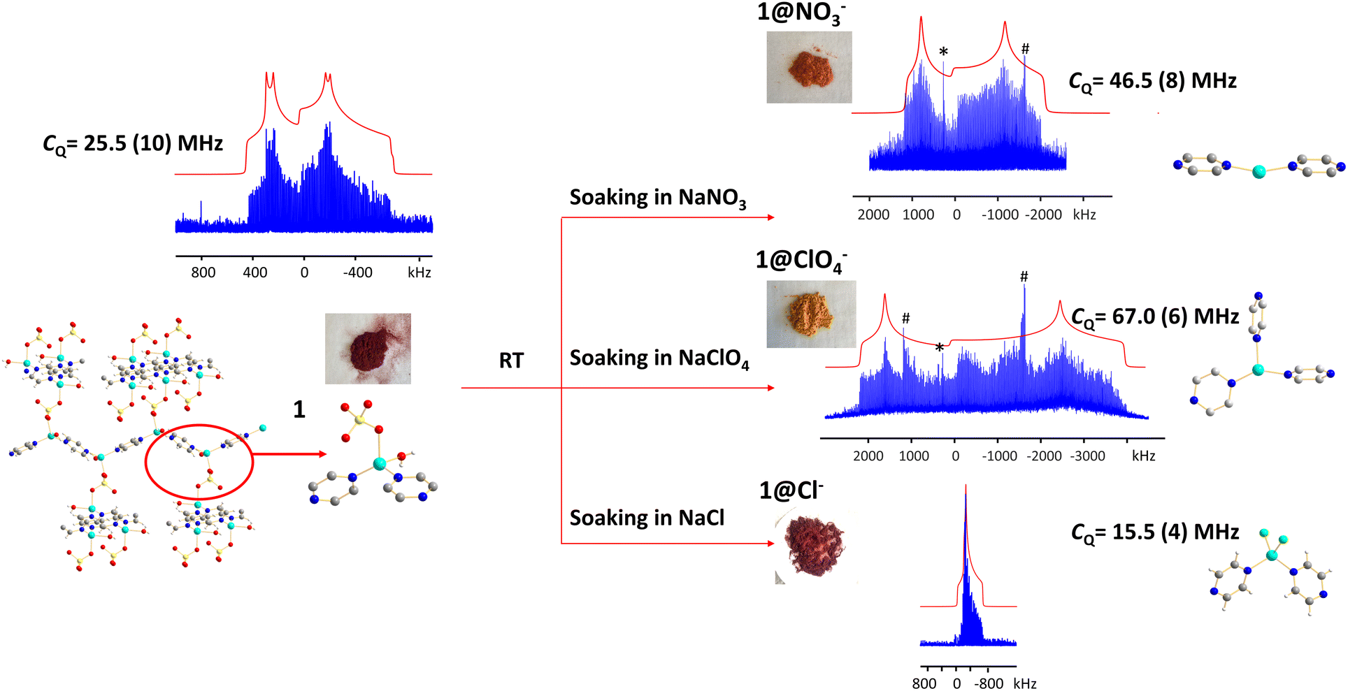 | ||
| Fig. 12 The 65Cu solid-state NMR spectra of 1 (Cu2(SO4)(pyz)2(H2O)2) and associated products after exposure to different aqueous solutions, as measured at 9.4 T. The asterisk (*) denotes a signal from metallic copper (Cu0) and the pound (#) indicates a resonance from a by-product containing Cu2O. | ||
While 1 is stable in air and water, this material quickly turns from dark red to orange when exposed to aqueous NaNO3 solution, yielding 1@NO3−. A white insoluble precipitate is evident when BaCl2/HCl is added, indicating that a migration of SO42− from 1 into solution has occurred. As a soft acid, the Cu(I) ion prefers to coordinate with the soft base of nitrogen rather than the hard base of oxygen, which explains the formation of a precipitate. The 65Cu NMR spectrum of 1@NO3− is a much broader ca. 3 MHz, which corresponds to a CQ(65Cu) of 46.5(8) MHz and a ηQ of 0.28(5) (Fig. 12). Using Fig. 10 as a guide, the significant increase in CQ(65Cu) from 1 to 1@NO3− indicates that the local coordination at Cu has changed from four-coordinate to two- or three-coordinate. When 1 was immersed in a NaClO4 solution, the powder changed to an orange-yellow color, and the resulting product was termed 1@ClO4−. The 65Cu NMR spectrum of 1@ClO4− at 9.4 T has an impressive breadth of ca. 7 MHz, with a CQ(65Cu) of 67.0(6) MHz and ηQ of 0.23(7); the increase in CQ again indicates that Cu now resides in a two- or three-coordinate local environment. When 1 is exposed to aqueous NaCl, the original dark red color is retained, however, the 65Cu NMR spectral breadth is considerably narrowed and the lineshape is altered in a distinct fashion. The 1@Cl− compound corresponds to a decreased CQ(65Cu) of 15.5(4) MHz, which indicates that the four-coordinate tetrahedral geometry is preserved at Cu, along with a significantly increased ηQ of 0.98(2). The well-defined 65Cu NMR powder patterns of 1 after exposure to NO3−, ClO4− and Cl− indicates that the local structure about Cu is relatively ordered in all instances. Using the estimated Cu coordination states obtained from the various 65Cu NMR spectra of 1 and its derivatives in mind, a search of the CCDC database was performed for any structures potentially matching or similar to the anion-exchanged products obtained in this study. Three compounds were identified: {Cu(pyz)(NO3)}n which contains a two-coordinate CuN2 moiety,105 {Cu(pyz)1.5(ClO4)}n with a three-coordinate CuN3 local structure,105 and {CuCl(pyz)}n with a four-coordinate CuCl2N2 environment.106 The reported structures had been synthesized independently through solvothermal routes, and not via the anion-exchange approach we employed.
The experimental PXRD patterns of 1@NO3−, 1@ClO4−, 1@Cl−, along with the calculated PXRD patterns of {Cu(pyz)(NO3)}n, {Cu(pyz)1.5(ClO4)}n, and {CuCl(pyz)}n from the reported solvothermal approaches are shown in Fig. S22.† The experimental PXRD pattern of 1@Cl− matches perfectly with the calculated pattern of {CuCl(pyz)}n, indicating the anion-exchanged product 1@Cl− is identical to solvothermally synthesized {CuCl(pyz)}n. This also confirms that a four-coordinate Cu(I) tetrahedral environment exists in 1@Cl−, as predicted from CQ(65Cu) NMR values. In contrast, the PXRD patterns of anion-exchanged 1@NO3− and 1@ClO4− look similar to those of solvothermally synthesized {Cu(pyz)(NO3)}n and {Cu(pyz)1.5(ClO4)}n, but are not identical. It appears that the pairs of 1@NO3− and {Cu(pyz)(NO3)}n MOFs, and the 1@ClO4−, and {Cu(pyz)1.5(ClO4)}n MOFs, are of similar connectivities but reside in different crystal structures (i.e., space groups). The Cu(I) coordination numbers are two and three in {Cu(pyz)(NO3)}n and {Cu(pyz)1.5(ClO4)}n, respectively, which is consistent with expectations based on the experimental 1@NO3− and 1@ClO4−CQ(65Cu) values. The Cu(I) center is generally considered to be a soft acid, and preferentially binds with soft base ligands such as N donors and halogen ions, rather than with hard bases such as O donors. In good agreement, we observed that the formation of 1@Cl− from 200 mg of 1 in a saturated aqueous solution concluded within ca. 30 min. In the context of hard and soft acids and bases, the cleavage of Cu(I)–O bonds to H2O and SO42− and the formation of Cu(I)–Cl bonds to yield a CuCl2N2 tetrahedral coordination environment in 1@Cl− is favorable and should proceed quickly. In a similar finding, the reaction of 1 with NO3− was also noted to conclude within 30 min; the zig-zag one-dimensional chains are sufficiently stable enough to exist without sulfate ions or coordinated water molecules, which then yields a two-coordinated Cu(I)N2 configuration with NO3− solely as a charge balancing anion. In stark contrast, the formation of 1@ClO4− requires ca. 12 hours of reaction time. After the cleavage of Cu–O bonds to H2O and SO42−, the formation of Cu–N bonds to pyrazine linkers in a new trigonal geometry requires a much longer duration because perchlorate is a very weakly coordinating anion and is not directly bound to Cu(I).
Conclusions
A series of Cu(I)-containing MOFs featuring Cu sites in different coordination environments have been examined using 63/65Cu ultra-wideline NMR and DFT calculations. The diversity of local environments of Cu(I) centers in MOFs leads to CQ(65Cu) values ranging from 18.8 to 74.8 MHz, which are diagnostic of the local Cu coordination environment and geometry. Multiple broad and overlapping 63/65Cu NMR signals arising from several unique Cu sites in MOFs can be resolved under favorable situations, and then simulated to extract information on the Cu local environment.63/65Cu NMR spectroscopy provides direct evidence regarding the evolution of local Cu environments during MOF structural transformation processes. The sensitivity of this technique can also be exploited to monitor and characterize MOF phase transitions. Even in the challenging case of Cu(I/II) mixed valence MOFs, 63/65Cu NMR spectra can be obtained, and are influenced by paramagnetic interactions when Cu(I) is especially proximate to Cu(II). We have proven 63/65Cu NMR can be performed within reasonable experimental times at a lower magnetic field of 9.4 T despite the weight dilution of Cu(I) centers in MOFs. DFT-calculated 63/65Cu EFG tensor parameters have been presented and rigorously compared with experimental values; calculations using geometry-optimized structures generally lead to better agreement with experimental results except for two instances, and the origins of these disagreements were explored. We have established a list of CQ(Cu) values from this and previous studies that permits estimation of local Cu coordination using only the CQ value, which is broadly applicable to many other Cu systems. This study highlights the versatility of 63/65Cu solid-state NMR, extending its relevance beyond MOFs and towards any chemical systems containing either abundant or dilute Cu(I) centers, with applications in fields such as catalysis, surface chemistry, solar cells, and biochemistry.
Materials and Methods
Sample preparation
The reported procedures were followed for MOF synthesis when possible.12–16,18,65,107 All details regarding synthesis and non-NMR characterization of the Cu compounds can be found in the ESI.†Solid-state NMR experiments
In general, 63/65Cu NMR spectra were acquired under static conditions using the solid echo or WURST-CPMG (Wideband Uniform Rate Smooth Truncation-Carr Purcell Meiboom Gill)100,108 pulse sequences. Solid echo experiments give rise to a smooth continuous lineshape, while WURST-CPMG experiments concentrate the signal into discrete spikelets that trace out the overall manifold of the powder pattern. Most of the ultra-wideline 63/65Cu NMR spectra in this work were too broad to be acquired in a single experiment, which necessitated the use of the VOCS (variable-offset cumulative spectra) method.109 The VOCS approach involves acquiring several sub-spectra at evenly spaced transmitter offsets using otherwise identical experimental parameters, and then co-adding the subspectra together to obtain the total 63/65Cu NMR spectrum. All 63Cu and 65Cu NMR spectra were referenced to solid CuCl at 0 ppm.NMR simulations
Extraction of NMR parameters was performed using the WSolids software package.110 The experimental error bounds for each measured parameter were determined by visual comparison of simulated spectra; the parameter in question was varied bidirectionally from the best-fit value, keeping other parameters constant, until differences were observed. The reader is directed towards the “NMR interactions and NMR parameters” section in the ESI† for a discussion of NMR interactions.Quantum chemical calculations
The CASTEP Academic Release version code 19.11111 was used to calculate 65Cu magnetic shielding and electric field gradient (EFG) tensor parameters via ab initio plane-wave density functional theory (DFT) methods. Calculations were performed on the SHARCNET computational network (https://www.sharcnet.ca/). Perdew, Burke, and Ernzerhof (PBE) functionals were employed with the generalized gradient approximation (GGA)112 for the exchange correlation energy in all instances, with a plane-wave basis set cutoff energy of 800 eV. NMR parameters were calculated using “on-the-fly” ultrasoft pseudopotentials and the gauge-including projector-augmented wave (GIPAW) formalism.113,114 The DFT CQ (MHz) values were obtained from calculated EFG tensor parameters using the most recently reported 63/65Cu quadrupole moment.57 The calculated 63Cu and 65Cu magnetic (chemical) shielding values (σ) in each MOF were converted to the corresponding chemical shift (δ) values using the formula δiso = σref − σiso. Note that σref is the 63/65Cu shielding for the reference sample CuCl(s), where σref (CuCl(s)) was calculated to be 702.68 ppm. Further details regarding geometry optimization schemes, along with the software and methodology used for cluster DFT calculations, can be found in the ESI.†
EFG tensor analysis
The EFG tensor has three principal components denoted V11, V22, and V33, defined such that |V33| ≥ |V22| ≥ |V11|. The agreement between experimental Vexpkk, k = 1, 2, 3 and Vcalkk, k = 1, 2, 3 can be evaluated using the EFG distance metric Γ86,93 (in atomic units, a.u.). Please see the ESI† for a detailed explanation of EFG tensor parameters and Γ.Author contributions
W. Z.: conceptualization, investigation, formal analysis, methodology, computation, writing, review, editing; B. E. G. L.: writing, review, editing; V. V. T.: investigation, review, editing; S. C.: investigation; Y. H.: conceptualization, resources, funding, formal analysis, writing, review, editing.Conflicts of interest
The authors declare no conflicts of interest.Acknowledgements
Y. H. thanks the Natural Science and Engineering Research Council (NSERC) of Canada for a Discovery Grant. Access to the 21.1 T NMR spectrometer was provided by the Government of Canada Ultrahigh-Field NMR Collaboration Platform, operated by the National Research Council of Canada with support from Laboratories Canada, and a consortium of other Canadian Government Departments and Universities. We thank Dr Mathew Willans at the J. B. Stothers NMR Facility (University of Western Ontario) for his assistance with 65Cu WURST-CPMG NMR experiments at 9.4 T. This work was made possible by the facilities of the Shared Hierarchical Academic Research Computing Network (SHARCNET: http://www.sharcnet.ca), Compute/Calcul Canada, and the Digital Research Alliance of Canada.References
- S. Kitagawa, Chem. Soc. Rev., 2014, 43, 5415–5418 RSC.
- H. Furukawa, K. E. Cordova, M. O'Keeffe and O. M. Yaghi, Science, 2013, 341, 1230444 CrossRef PubMed.
- P. Nugent, Y. Belmabkhout, S. D. Burd, A. J. Cairns, R. Luebke, K. Forrest, T. Pham, S. Ma, B. Space and L. Wojtas, Nature, 2013, 495, 80–84 CrossRef CAS PubMed.
- K. Sumida, D. L. Rogow, J. A. Mason, T. M. McDonald, E. D. Bloch, Z. R. Herm, T.-H. Bae and J. R. Long, Chem. Rev., 2012, 112, 724–781 CrossRef CAS PubMed.
- J. Della Rocca, D. Liu and W. Lin, Acc. Chem. Res., 2011, 44, 957–968 CrossRef CAS PubMed.
- M. Dincă and J. R. Long, Chem. Rev., 2020, 120, 8037–8038 CrossRef.
- M. Eddaoudi, D. B. Moler, H. Li, B. Chen, T. M. Reineke, M. O’keeffe and O. M. Yaghi, Acc. Chem. Res., 2001, 34, 319–330 CrossRef CAS PubMed.
- J. Ha, J. H. Lee and H. R. Moon, Inorg. Chem. Front., 2020, 7, 12–27 RSC.
- R. Peng, M. Li and D. Li, Coord. Chem. Rev., 2010, 254, 1–18 CrossRef CAS.
- D. Shi, R. Zheng, M. Sun, X. Cao, C. Sun, C. Cui, C. Liu, J. Zhao and M. Du, Angew. Chem., Int. Ed., 2017, 129, 14829–14833 CrossRef.
- L. Chen, X. Chen, R. Ma, K. Lin, Q. Li, J.-P. Lang, C. Liu, K. Kato, L. Huang and X. Xing, J. Am. Chem. Soc., 2022, 144, 13688–13695 CrossRef CAS PubMed.
- D. Braga, L. Maini, P. P. Mazzeo and B. Ventura, Chem.–Eur. J., 2010, 16, 1553–1559 CrossRef CAS PubMed.
- A. A. García-Valdivia, F. J. Romero, J. Cepeda, D. P. Morales, N. Casati, A. J. Mota, L. A. Zotti, J. J. Palacios, D. Choquesillo-Lazarte and J. F. Salmerón, Chem. Commun., 2020, 56, 9473–9476 RSC.
- X. Zhou, J. Dong, Y. Zhu, L. Liu, Y. Jiao, H. Li, Y. Han, K. Davey, Q. Xu and Y. Zheng, J. Am. Chem. Soc., 2021, 143, 6681–6690 CrossRef CAS PubMed.
- O. M. Yaghi and H. Li, J. Am. Chem. Soc., 1995, 117, 10401–10402 CrossRef CAS.
- O. M. Yaghi and G. Li, Angew. Chem., Int. Ed., 1995, 34, 207–209 CrossRef CAS.
- J.-J. Wang, X. Mao, J.-N. Yang, Y.-C. Yin, J.-S. Yao, L.-Z. Feng, F. Zhu, C. Ma, C. Yang and G. Zou, Nano Lett., 2021, 21, 4115–4121 CrossRef CAS PubMed.
- H. Fei, D. L. Rogow and S. R. J. Oliver, J. Am. Chem. Soc., 2010, 132, 7202–7209 CrossRef CAS.
- V. Martins, J. Xu, X. Wang, K. Chen, I. Hung, Z. Gan, C. Gervais, C. Bonhomme, S. Jiang, A. Zheng, B. E. G. Lucier and Y. Huang, J. Am. Chem. Soc., 2020, 142, 14877–14889 CrossRef CAS PubMed.
- B. E. G. Lucier, S. Chen and Y. Huang, Acc. Chem. Res., 2018, 51, 319–330 CrossRef CAS PubMed.
- S. Chen, Z. Song, J. Lyu, Y. Guo, B. E. G. Lucier, W. Luo, M. S. Workentin, X. Sun and Y. Huang, J. Am. Chem. Soc., 2020, 142, 4419–4428 CrossRef CAS PubMed.
- E. Brunner and M. Rauche, Chem. Sci., 2020, 11, 4297–4304 RSC.
- C. He, S. Li, Y. Xiao, J. Xu and F. Deng, Solid State Nucl. Magn. Reson., 2022, 117, 101772 CrossRef CAS PubMed.
- H. C. Hoffmann, M. Debowski, P. Müller, S. Paasch, I. Senkovska, S. Kaskel and E. Brunner, Materials, 2012, 5, 2537–2572 CrossRef CAS.
- V. J. Witherspoon, J. Xu and J. A. Reimer, Chem. Rev., 2018, 118, 10033–10048 CrossRef CAS PubMed.
- Y. Fu, H. Guan, J. Yin and X. Kong, Coord. Chem. Rev., 2021, 427, 213563 CrossRef CAS.
- J. Hou, M. L. Rios Gomez, A. Krajnc, A. McCaul, S. Li, A. M. Bumstead, A. F. Sapnik, Z. Deng, R. Lin and P. A. Chater, J. Am. Chem. Soc., 2020, 142, 3880–3890 CrossRef CAS.
- C. S. Vogelsberg, F. J. Uribe-Romo, A. S. Lipton, S. Yang, K. N. Houk, S. Brown and M. A. Garcia-Garibay, Proc. Natl. Acad. Sci. U.S.A., 2017, 114, 13613–13618 CrossRef CAS PubMed.
- R. S. K. Madsen, A. Qiao, J. Sen, I. Hung, K. Chen, Z. Gan, S. Sen and Y. Yue, Science, 2020, 367, 1473–1476 CrossRef CAS PubMed.
- C. A. O'Keefe, C. Mottillo, J. Vainauskas, L. Fábián, T. Friščić and R. W. Schurko, Chem. Mater., 2020, 32, 4273–4281 CrossRef.
- W. Zhang, S. Chen, V. V. Terskikh, B. E. G. Lucier and Y. Huang, Solid State Nucl. Magn. Reson., 2022, 119, 101793 CrossRef CAS PubMed.
- Y. Fu, Z. Kang, W. Cao, J. Yin, Y. Tu, J. Li, H. Guan, Q. Wang and X. Kong, Angew. Chem., Int. Ed., 2021, 133, 7798–7806 CrossRef.
- J. Yin, Z. Kang, Y. Fu, W. Cao, Y. Wang, H. Guan, Y. Yin, B. Chen, X. Yi and W. Chen, Nat. Commun., 2022, 13, 1–9 Search PubMed.
- B. E. G. Lucier, W. Zhang, A. Sutrisno and Y. Huang, A review of exotic quadrupolar metal NMR in MOFs, in Comprehensive Inorganic Chemistry III, ed. J. Reedijk and K. R. Poeppelmeier, Elsevier, 2023, pp. 330–365 Search PubMed.
- J. A. Tang, B. D. Ellis, T. H. Warren, J. V Hanna, C. L. B. Macdonald and R. W. Schurko, J. Am. Chem. Soc., 2007, 129, 13049–13065 CrossRef CAS PubMed.
- D. Rusanova, K. J. Pike, R. Dupree, J. V Hanna, O. N. Antzutkin, I. Persson and W. Forsling, Inorg. Chim. Acta, 2006, 359, 3903–3910 CrossRef CAS.
- G. A. Bowmaker, J. V Hanna, F. E. Hahn, A. S. Lipton, C. E. Oldham, B. W. Skelton, M. E. Smith and A. H. White, Dalton Trans., 2008, 13, 1710–1720 RSC.
- G. V. M. Williams and J. Haase, Phys. Rev. B, 2007, 75, 172506 CrossRef.
- F. Haarmann, M. Armbrüster and Y. Grin, Chem. Mater., 2007, 19, 1147–1153 CrossRef CAS.
- M. Kujime, T. Kurahashi, M. Tomura and H. Fujii, Inorg. Chem., 2007, 46, 541–551 CrossRef CAS PubMed.
- T. J. Bastow and S. Celotto, Acta Mater., 2003, 51, 4621–4630 CrossRef CAS.
- S. Sakida, N. Kato and Y. Kawamoto, Mater. Res. Bull., 2002, 37, 2263–2274 CrossRef CAS.
- G. Brunklaus, J. C. C. Chan, H. Eckert, S. Reiser, T. Nilges and A. Pfitzner, Phys. Chem. Chem. Phys., 2003, 5, 3768–3776 RSC.
- D. Rusanova, K. J. Pike, I. Persson, R. Dupree, M. Lindberg, J. V Hanna, O. N. Antzutkin and W. Forsling, Polyhedron, 2006, 25, 3569–3580 CrossRef CAS.
- D. Rusanova, K. J. Pike, I. Persson, J. V Hanna, R. Dupree, W. Forsling and O. N. Antzutkin, Chem.–Eur. J., 2006, 12, 5282–5292 CrossRef CAS PubMed.
- D. Rusanova, W. Forsling, O. N. Antzutkin, K. J. Pike and R. Dupree, Langmuir, 2005, 21, 4420–4424 CrossRef CAS PubMed.
- D. Rusanova, W. Forsling, O. N. Antzutkin, K. J. Pike and R. Dupree, J. Magn. Reson., 2006, 179, 140–145 CrossRef CAS PubMed.
- S. Mazumdar, Phys. Rev. B, 2018, 98, 205153 CrossRef CAS.
- S. Hu, J. A. Reimer and A. T. Bell, J. Phys. Chem. B, 1997, 101, 1869–1871 CrossRef CAS.
- L. Choubrac, M. Paris, A. Lafond, C. Guillot-Deudon, X. Rocquefelte and S. Jobic, Phys. Chem. Chem. Phys., 2013, 15, 10722–10725 RSC.
- B. E. G. Lucier, J. A. Tang, R. W. Schurko, G. A. Bowmaker, P. C. Healy and J. V Hanna, J. Phys. Chem. C, 2010, 114, 7949–7962 CrossRef CAS.
- S. Perruchas, Dalton Trans., 2021, 50, 12031–12044 RSC.
- A. Bhattacharya, D. G. Tkachuk, A. Mar and V. K. Michaelis, Chem. Mater., 2021, 33, 4709–4722 CrossRef CAS.
- A. Bhattacharya, V. Mishra, D. G. Tkachuk, A. Mar and V. K. Michaelis, Phys. Chem. Chem. Phys., 2022, 24, 24306–24316 RSC.
- S. Kroeker and R. E. Wasylishen, Can. J. Chem., 1999, 77, 1962–1972 CrossRef CAS.
- H. Yu, X. Tan, G. M. Bernard, V. V Terskikh, J. Chen and R. E. Wasylishen, J. Phys. Chem. A, 2015, 119, 8279–8293 CrossRef CAS PubMed.
- N. J. Stone, At. Data Nucl. Data Tables, 2016, 111, 1–28 CrossRef.
- P. Pyykkö, Mol. Phys., 2018, 116, 1328–1338 CrossRef.
- J. Meija, T. B. Coplen, M. Berglund, W. A. Brand, P. De Bièvre, M. Gröning, N. E. Holden, J. Irrgeher, R. D. Loss and T. Walczyk, Pure Appl. Chem., 2016, 88, 293–306 CrossRef CAS.
- R. K. Harris, E. D. Becker, S. M. C. de Menezes, R. Goodfellow and P. Granger, Pure Appl. Chem., 2001, 73, 1795–1818 CrossRef CAS.
- R. W. Schurko, Acc. Chem. Res., 2013, 46, 1985–1995 CrossRef CAS PubMed.
- S. S. Nagarkar, H. Kurasho, N. T. Duong, Y. Nishiyama, S. Kitagawa and S. Horike, Chem. Commun., 2019, 55, 5455–5458 RSC.
- J. Xu, B. E. G. Lucier, R. Sinelnikov, V. V Terskikh, V. N. Staroverov and Y. Huang, Chem.–Eur. J., 2015, 21, 14348–14361 CrossRef CAS PubMed.
- S. K. Ramakrishna, K. Kundu, J. K. Bindra, S. A. Locicero, D. R. Talham, A. P. Reyes, R. Fu and N. S. Dalal, J. Phys. Chem. C, 2021, 125, 3441–3450 CrossRef CAS.
- C. Näther and I. Jeß, Monatsh. fur Chem., 2001, 132, 897–910 CrossRef.
- O. M. Yaghi, M. O'Keeffe, N. W. Ockwig, H. K. Chae, M. Eddaoudi and J. Kim, Nature, 2003, 423, 705–714 CrossRef CAS PubMed.
- C. Cappuccino, F. Farinella, D. Braga and L. Maini, Cryst. Growth Des., 2019, 19, 4395–4403 CrossRef CAS.
- F. A. Perras and D. L. Bryce, Angew. Chem., Int. Ed., 2012, 51, 4227–4230 CrossRef CAS PubMed.
- K. E. Johnston, C. A. O'Keefe, R. M. Gauvin, J. Trébosc, L. Delevoye, J. Amoureux, N. Popoff, M. Taoufik, K. Oudatchin and R. W. Schurko, Chem.–Eur. J., 2013, 19, 12396–12414 CrossRef CAS PubMed.
- Y. Gao, L. Zhang, Y. Gu, W. Zhang, Y. Pan, W. Fang, J. Ma, Y.-Q. Lan and J. Bai, Chem. Sci., 2020, 11, 10143–10148 RSC.
- X. Jiang, Y. Jiao, S. Hou, L. Geng, H. Wang and B. Zhao, Angew. Chem., Int. Ed., 2021, 133, 20580–20586 CrossRef.
- S. Demir, H. M. Çepni, N. Bilgin, M. Hołyńska and F. Yilmaz, Polyhedron, 2016, 115, 236–241 CrossRef CAS.
- C. H. Hendon and A. Walsh, Chem. Sci., 2015, 6, 3674–3683 RSC.
- M. Todaro, G. Buscarino, L. Sciortino, A. Alessi, F. Messina, M. Taddei, M. Ranocchiari, M. Cannas and F. M. Gelardi, J. Phys. Chem. C, 2016, 120, 12879–12889 CrossRef CAS.
- H. E. L. Mkami, M. I. H. Mohideen, C. Pal, A. McKinlay, O. Scheimann and R. E. Morris, Chem. Phys. Lett., 2012, 544, 17–21 CrossRef.
- L. M. B. Napolitano, O. R. Nascimento, S. Cabaleiro, J. Castro and R. Calvo, Phys. Rev. B: Condens. Matter Mater. Phys., 2008, 77, 214423 CrossRef.
- M. Simenas, M. Kobalz, M. Mendt, P. Eckold, H. Krautscheid, J. Banys and A. Pöppl, J. Phys. Chem. C, 2015, 119, 4898–4907 CrossRef CAS.
- A. Pöppl, S. Kunz, D. Himsl and M. Hartmann, J. Phys. Chem. C, 2008, 112, 2678–2684 CrossRef.
- A. J. Pell, G. Pintacuda and C. P. Grey, Prog. Nucl. Magn. Reson. Spectrosc., 2019, 111, 1–271 CrossRef CAS PubMed.
- M. Bertmer, Solid State Nucl. Magn. Reson., 2017, 81, 1–7 CrossRef CAS PubMed.
- X. Kong, V. V Terskikh, R. L. Khade, L. Yang, A. Rorick, Y. Zhang, P. He, Y. Huang and G. Wu, Angew. Chem., Int. Ed., 2015, 54, 4753–4757 CrossRef CAS PubMed.
- V. I. Bakhmutov, Chem. Rev., 2011, 111, 530–562 CrossRef CAS PubMed.
- L. J. M. Davis, I. Heinmaa, B. L. Ellis, L. F. Nazar and G. R. Goward, Phys. Chem. Chem. Phys., 2011, 13, 5171–5177 RSC.
- M. Kondo, T. Yoshitomi, H. Matsuzaka, S. Kitagawa and K. Seki, Angew. Chem., Int. Ed., 1997, 36, 1725–1727 CrossRef CAS.
- G. A. Bowmaker, A. V Churakov, R. K. Harris, J. A. K. Howard and D. C. Apperley, Inorg. Chem., 1998, 37, 1734–1743 CrossRef CAS.
- S. T. Holmes and R. W. Schurko, J. Phys. Chem. C, 2018, 122, 1809–1820 CrossRef CAS.
- J. Cui, T. R. Prisk, D. L. Olmsted, V. Su, M. Asta and S. E. Hayes, Chem.–Eur. J., 2023, 29, e202203052 CrossRef CAS PubMed.
- F. A. Perras and D. L. Bryce, J. Phys. Chem. C, 2012, 116, 19472–19482 CrossRef CAS.
- P. Hodgkinson, Prog. Nucl. Magn. Reson. Spectrosc., 2020, 118, 10–53 CrossRef PubMed.
- C. Martineau-Corcos, Curr. Opin. Colloid Interface Sci., 2018, 33, 35–43 CrossRef CAS.
- R. K. Harris, R. E. Wasylishen and M. J. Duer, NMR Crystallography, John Wiley & Sons, 2009, vol. 4 Search PubMed.
- S. E. Ashbrook and D. McKay, Chem. Commun., 2016, 52, 7186–7204 RSC.
- S. T. Holmes, C. S. Vojvodin and R. W. Schurko, J. Phys. Chem. A, 2020, 124, 10312–10323 CrossRef CAS PubMed.
- C. M. Widdifield and D. L. Bryce, Phys. Chem. Chem. Phys., 2009, 11, 7120–7122 RSC.
- J. R. Yates, C. J. Pickard, M. C. Payne, R. Dupree, M. Profeta and F. Mauri, J. Phys. Chem. A, 2004, 108, 6032–6037 CrossRef CAS.
- F. Alkan, S. T. Holmes, R. J. Iuliucci, K. T. Mueller and C. Dybowski, Phys. Chem. Chem. Phys., 2016, 18, 18914–18922 RSC.
- S. T. Holmes, S. Bai, R. J. Iuliucci, K. T. Mueller and C. Dybowski, J. Comput. Chem., 2017, 38, 949–956 CrossRef CAS PubMed.
- S. T. Holmes and R. W. Schurko, J. Chem. Theory Comput., 2019, 15, 1785–1797 CrossRef CAS PubMed.
- S. T. Holmes, R. J. Iuliucci, K. T. Mueller and C. Dybowski, J. Chem. Theory Comput., 2015, 11, 5229–5241 CrossRef CAS PubMed.
- L. A. O'Dell, A. J. Rossini and R. W. Schurko, Chem. Phys. Lett., 2009, 468, 330–335 CrossRef.
- I. R. Colinas, K. K. Inglis, F. Blanc and S. R. J. Oliver, Dalton Trans., 2017, 46, 5320–5325 RSC.
- L.-L. Li, X.-Q. Feng, R.-P. Han, S.-Q. Zang and G. Yang, J. Hazard. Mater., 2017, 321, 622–628 CrossRef CAS PubMed.
- K. Uemura, A. Maeda and H. Kita, Polyhedron, 2008, 27, 2939–2942 CrossRef CAS.
- P. Amo-Ochoa, G. Givaja, P. J. S. Miguel, O. Castillo and F. Zamora, Inorg. Chem. Commun., 2007, 10, 921–924 CrossRef CAS.
- S. Mohapatra and T. K. Maji, Dalton Trans., 2010, 39, 3412–3419 RSC.
- J. M. Moreno, J. Suarez-Varela, E. Colacio, J. C. Avila-Rosón, M. A. Hidalgo and D. Martin-Ramos, Can. J. Chem., 1995, 73, 1591–1595 CrossRef CAS.
- S. Qi, X. Qian, Q. He, K. Miao, Y. Jiang, P. Tan, X. Liu and L. Sun, Angew. Chem., Int. Ed., 2019, 58, 10104–10109 CrossRef CAS PubMed.
- L. A. O'Dell, Mod. Magn. Reson., 2017, 56, 1–22 CrossRef.
- D. Massiot, I. Farnan, N. Gautier, D. Trumeau, A. Trokiner and J. P. Coutures, Solid State Nucl. Magn. Reson., 1995, 4, 241–248 CrossRef CAS PubMed.
- K. Eichele and R. E. Wasylishen, WSolids1, Version 1.19.11, Univ. Tübingen, Tübingen, Ger, 2009 Search PubMed.
- S. J. Clark, M. D. Segall, C. J. Pickard, P. J. Hasnip, M. I. J. Probert, K. Refson and M. C. Payne, Z. fur Krist. – Cryst. Mater., 2005, 220, 567–570 CrossRef CAS.
- J. P. Perdew, K. Burke and M. Ernzerhof, Phys. Rev. Lett., 1996, 77, 3865 CrossRef CAS PubMed.
- J. R. Yates, C. J. Pickard and F. Mauri, Phys. Rev. B: Condens. Matter Mater. Phys., 2007, 76, 024401 CrossRef.
- C. J. Pickard and F. Mauri, Phys. Rev. B: Condens. Matter Mater. Phys., 2001, 63, 245101 CrossRef.
Footnote |
| † Electronic supplementary information (ESI) available. See DOI: https://doi.org/10.1039/d4sc00782d |
| This journal is © The Royal Society of Chemistry 2024 |