
 Open Access Article
 This Open Access Article is licensed under a Creative Commons Attribution-Non Commercial 3.0 Unported Licence
Methods for the analysis, interpretation, and prediction of single-molecule junction conductance behaviour
Elena
Gorenskaia
and
Paul J.
Low
 *
*
School of Molecular Sciences, University of Western Australia, 35 Stirling Highway, Crawley, Western Australia 6026, Australia. E-mail: paul.low@uwa.edu.au
First published on 25th May 2024
Abstract
This article offers a broad overview of measurement methods in the field of molecular electronics, with a particular focus on the most common single-molecule junction fabrication techniques, the challenges in data analysis and interpretation of single-molecule junction current–distance traces, and a summary of simulations and predictive models aimed at establishing robust structure–property relationships of use in the further development of molecular electronics.
1. Introduction
The field of molecular electronics has matured and evolved over the past decades from an initial focus on the mimicry of solid-state electronic components to emerging applications in molecular materials science.1,2 New sub-areas in molecular electronics are advancing rapidly, and in recent years examples including supramolecular electronics,3 single-molecule bioelectronics,4 single-supramolecule electronics,5 and single-cluster electronics6 can be identified. However, regardless of the ultimate application, molecular electronics can be broadly described as the science associated with, and technology arising from, the use of molecules as functional units carrying electrical charge between two macroscopic electrodes. Consequently, the basic tool for explorations in molecular electronics is an electrode|molecule|electrode system, or ‘molecular junction’ (Fig. 1). Molecular junctions can be formed from single molecules, molecular bundles or by contacting large numbers of molecules contained within molecular monolayers. However, the single-molecule junction is a unique platform for the collection of data that informs fundamental understanding of charge transport and chemical principles of structure–conductivity relationships in molecular electronics.7,8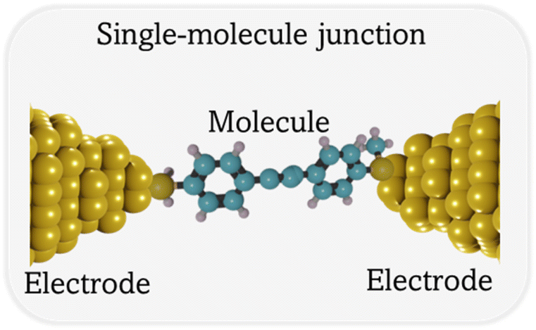 | ||
| Fig. 1 Schematic of a single-molecule junction. | ||
Creating single-molecule junctions requires sophisticated experimental techniques, and powerful methods have been developed to characterize and manipulate the conductance properties of single molecules through chemical, electrochemical, optical, mechanical, or environmental ‘gating’.2 In each of these methods, a molecule is initially trapped within a small electrode gap, and the current through the junction measured, often as the electrodes are drawn away from each other. Current flowing through the molecule within the junction gives a deviation from the exponential decay of current between the electrodes with the through-space separation, and the resulting current–distance plots contain plateaus characteristic of the molecular conductance. Such data are collected from many thousands of replicate measurements and analysed, often in the form of conductance histograms, to give a most probable value of molecular conductance.
Perhaps the most common approaches that meet the requirements of successful formation of single-molecule junctions in a reproducible and reliable manner are the scanning tunnelling microscope break-junction (STM-BJ), in which the electrodes are formed from the STM tip and a conducting substrate surface,9–11 and the mechanically controllable break-junction (MCBJ), which creates atomically sharp electrodes by breaking a thin metallic wire.12–14 More recently, conductive atomic force microscope break junction (AFM-BJ) methods that can simultaneously measure force and electrical signal have become increasingly popular.15
Each of these methods provide reproducible conductance histograms but with a broad distribution of junction-to-junction conductance values, typically with a standard deviation in the range of at least one order of magnitude.16 It is now widely appreciated that the bridging molecule and the molecule–electrode contact may change orientation and geometry as the junction is stretched and evolved, leading to considerable variations in the conductance properties of each individual junction.17–20 Moreover, unexpected conductance features in current–distance plots, including a variety of length-dependent characteristics, overall slope of the current plateaus, as well as sudden jumps and drops in conductance can appear as a result of chemical and physical processes, including polymerisation, isomerization, redox switching, supramolecular interactions and other molecular phenomena, taking place within the junction.21–23
The diversity of conductance features collected during the single-molecule junction experiment makes it difficult to model the junction formation and evolution processes that lead to the overall histogram, and discover and explore hidden sub-populations in aggregated data.24 Machine learning (ML) offers a solution for deep analysis of the stochastic nature of the junction-forming process and to extract events associated with other chemical or physical events that take place within the junction.25 The machine learning methods used for single-molecule conductance data analysis are broadly distinguished by the supervised or unsupervised algorithms upon which they are based. The main difference between these two approaches is the need for a manually labelled training set for supervised learning. However, the powerful nature of automated analysis based on ML comes with numerous pitfalls that require considered application and robust testing to ensure realistic results that are, of course, ultimately subject to human interpretation.25
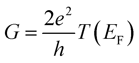
The underlying physical mechanisms and processes impinging on single-molecule junction conductance data are commonly explored using computational methods. Different theoretical models and computational approaches are used to analyse coherent (tunnelling)26 or incoherent (hopping)27 electron transport in molecular junctions. For coherent transport, the Landauer–Büttiker formalism (eqn (1)) can be used to calculate the conductance of a molecular junction.
 | (1) |
 , plots of the transmission function provide a convenient proxy measure for assessing relative molecular conductance features.
Beyond single-channel coherent tunnelling, quantum interference (QI) effects in molecular junctions have been identified and can significantly influence the shape of electron transmission function. QI arises from the wave-like nature of electrons that take multiple paths from the injection point at one electrode through the molecular scaffold to the collection point at the other. The emergent waves can interfere constructively, giving rise to broad, relatively high conductance region in the T(E) vs. E plot, or destructively, resulting in a pronounced ‘dip’ in the transmission function.30 It should be noted that whilst the probability of electron transmission through the molecule, including QI effects, can be calculated using density functional theory (DFT), which correctly predict trends in transport properties, DFT methods typically significantly under-estimate the HOMO–LUMO gap and therefore over-estimate the value of the conductance.31–33
For incoherent transport, hopping models are used to describe the motion of electrons through the molecular junction. These models assume that electrons move through the molecule by tunnelling between a sequence of adjacent sites in a step-wise fashion, rather than one-step tunnelling through the entire length of the molecule. Marcus theory, which describes charge transfer in terms of the energy difference between donor and acceptor states and the reorganization energy of the system, can be used as the basis for each step in a hopping model.34 Unlike the Landauer–Büttiker formalism, Marcus theory does not rely on quantum mechanical methods, but rather rests on classical assumptions about the behaviour of electrons and the energy landscape of the system.
An alternative, empirical method for prediction of molecular conductance in the coherent (tunnelling) electron transport regime leads to recently proposed Quantum Circuit Rules (QCR).35–38 The QCR based model describes the molecular junction as a series of weakly coupled scattering regions, and applies to non-resonant tunnel junctions with the Fermi energy of the electrodes near the middle of the transport resonances in the transmission function arising from the HOMO and LUMO. For a molecule of general form X–B–Y, where X and Y are the anchor groups that bind the molecule to the left and right electrodes, and B is the molecular backbone, the QCR can predict the trend in transport properties using transferable numerical parameters (aX, aY, and bB) for building blocks (X, Y and B) of a molecule in a junction.
This overview will outline the most common single-molecule junction fabrication techniques including STM-BJ, MCBJ, and AFM-BJ (Section 2), provide a general analysis of current–distance traces in the context of different processes in the junction during measurements (Section 3), and describe the factors that influence junction formation probability (JFP; Section 4). Machine learning models for analysis of conductance data are summarised in Section 5, while Section 6 gives a brief overview of theoretical simulations for molecular electronics, including DFT methods (Section 6.1) and complementary QCR based approaches (Section 6.2).
2. Formation of single-molecule junctions
Investigating the electrical properties of a molecule requires the use of nanoscale electrodes in devices that can maintain the separation between them within the dimensions of a molecule. Whilst a wide variety of experimental methods that achieve the formation of molecular junctions are known,2,39,40 perhaps the two most widely used approaches that meet the requirements for successful formation of single-molecule junctions are the scanning tunnelling microscope break-junction (STM-BJ),9–11 which utilizes the piezo-controlled position of the STM tip relative to a conductive substrate surface, and the mechanically controllable break-junction (MCBJ),12–14 in which the electrodes are formed and separated by bending a thin metallic wire supported on a flexible substrate with a pushing rod. In the absence of a molecular bridge, a tunnelling current through the electrode gap, which decays exponentially with distance as the electrodes are separated, is observed. When a molecule bridges the gap between two electrodes then a deviation from this exponential decay is observed as a plateau in the current–distance of electrode separation plot. The current plateau arising from charge transport through the molecule within the junction persists (and often evolves) as the junction electrodes are separated. As the electrode separation reaches a point where the molecule can no longer span the increased electrode gap, the junction is cleaved, and current falls back to the through-space tunnelling limit. In both methods, a relatively low bias voltage between the electrodes is usually applied (typically chosen to be in the range 0.05–0.6 V) to avoid break-down of through-molecule conductance and emergence of significantly large direct tunnelling between two electrodes across to the small gap.41–43 Conductance measurements using these methods can be carried out in different environments including organic solvents, aqueous electrolyte, ionic liquid, air, and vacuum. It has been demonstrated that these environmental factors can have an impact on single-molecule conductance by tuning molecular energies relative to the effective electrode Fermi levels.41,44,45Closely allied with the STM-BJ and MCBJ methods, the conducting probe atomic force microscope break junction (AFM-BJ) has also begun to attract attention.46 This technique combines the laser system of the AFM with a current measurement circuit, which enables the measurement of both the forces and conductance during the break junction process, allowing simultaneous electrical and mechanical characterization of molecule as the junction evolves.
2.1 Scanning tunnelling microscope break junction (STM-BJ)
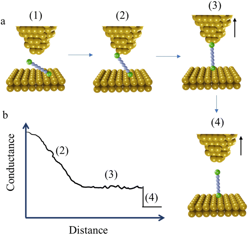
In the initial step of the STM-BJ experiment, the (gold) STM tip is crashed into the (gold) substrate to create a fused metal junction (Fig. 2a, Step 1). The tip is then withdrawn from the surface, pulling a metallic filament between the gold surface and tip. As the tip continues to withdraw the filament thins, evinced by stepwise drops in quantised conductance as the number of metal atoms in the junction decreases (i.e. nG0, where 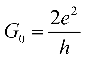 , the quantum of conductance), and ultimately breaks. This rupture causes the sudden generation of a nanoscale gap, typically measuring in the region of 5 Å, as a result of the ‘snap-back’ of the strained wire,47 leaving two atomically sharp electrodes (Fig. 2a, Step 2). This process is evinced by a consequent sharp drop from metal-atom point contact conductance (G0) to the exponentially distance dependant tunnelling current (Fig. 2a, Step 3). If the experiment is conducted in a dilute solution of the molecule of interest, these molecules can assemble along the exposed electrode surfaces, including the evolving metal filament.48 As the filament breaks, there is a possibility of trapping a molecule within the newly formed electrode gap to give the molecular junction (Fig. 2a, Step 4). As the tip continues to withdraw, eventually the junction length exceeds the geometric distance that can be spanned by the molecule, the junction ‘breaks’ and the current falls back to the direct tunnelling mechanism and decays exponentially until the noise of the instrument is reached (Fig. 2a, Step 5). The above steps are repeated several thousand times to give a statistically significant body of data. The resulting data can be displayed as a 1D histogram, where the most prominent peak reveals the most probable conductivity of the molecule (Fig. 2b), or as a 2D heat map or histogram49 where the dense conductance cloud represent single molecule features (Fig. 2c).
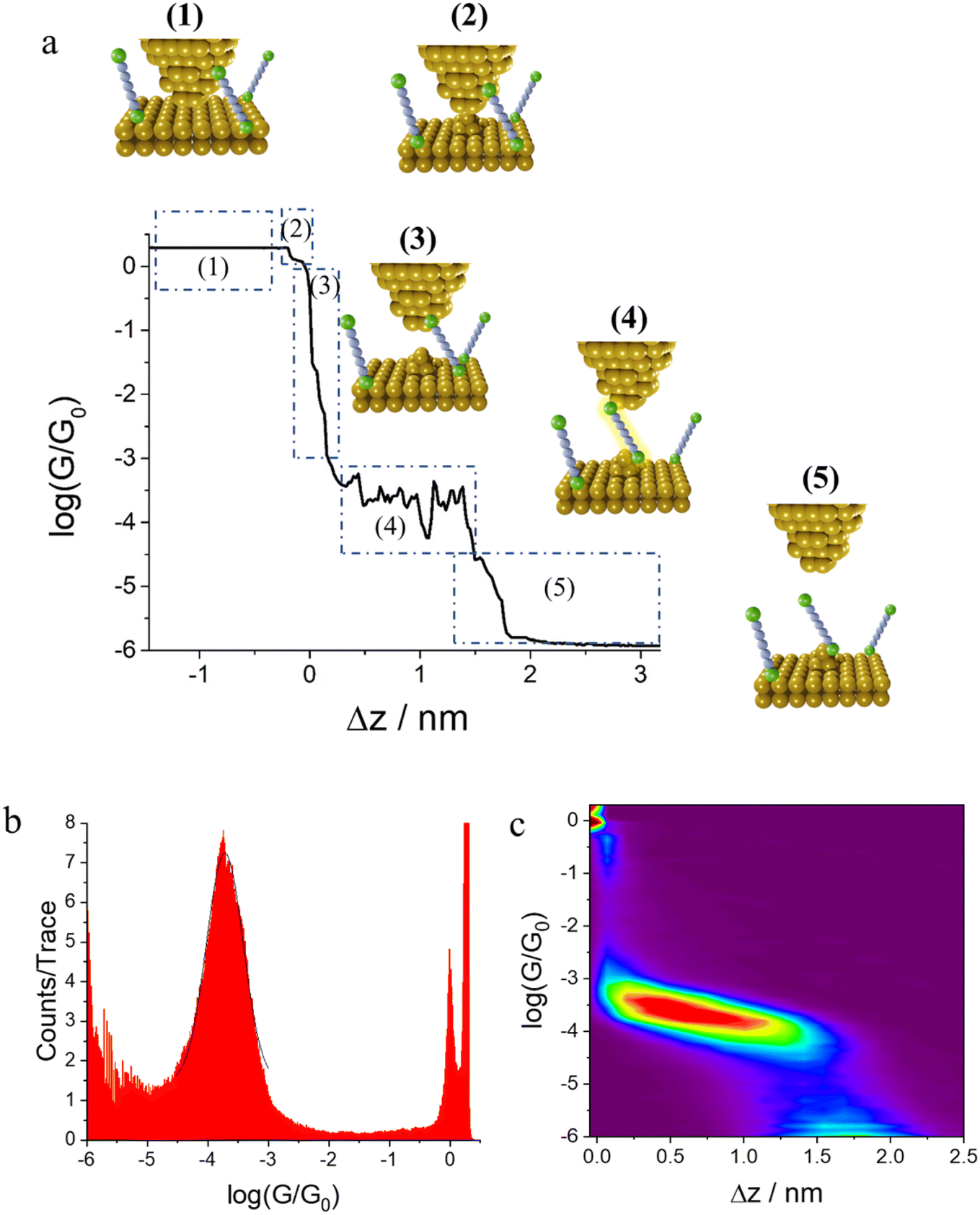 | ||
| Fig. 2 (a) A conductance–distance trace typical of the STM-BJ technique, annotated to illustrate the steps of molecular junction formation; (b) the corresponding 1D histogram comprised of ca. 2000 individual conductance traces; (c) the corresponding 2D conductance–distance heat-map (histogram) comprised by overlaying the individual conductance–distance traces where the false colour indicates the regions of greatest data density (red). | ||
Particular advantages of the STM-BJ technique include: the simplicity of fabrication using relatively readily available equipment, and the larger dimensions of the source and drain electrodes;50 the compatibility with measurements made within an electrochemical environment, allowing electrochemical addressing and gating of molecule within the junction;51 and the largely automated data collection process using commercial software and simple data output format.
The STM-BJ method mentioned earlier is sometimes referred to as the “tapping approach” because it involves measuring the single-molecule conductance by repeatedly creating and breaking the molecular junction through “tapping” the tip in and out of contact with the substrate surface.16 Beyond the STM-BJ, closely related techniques including current–distance spectroscopy (or I(s)) methods have been developed. The I(s), or “soft-tapping” method is similar to STM-BJ with the key distinctions being that an atomically sharp tip is used, and an initial set-point current is chosen to allow the tip to approach close to, but not touch, the substrate surface.52 The positioning of the STM tip just above the surface allows capture a molecule assembled on the surface within the newly formed junction, without making contact between the tip and substrate (Fig. 3a and b).53,54
 | ||
| Fig. 3 Schematic illustration of the I(s) or “soft tapping” technique: (a) the steps of molecular junction formation (in this technique molecular junctions are formed without first forming a tip-to-substrate contact); (b) typical conductance–distance trace of the “soft tapping” STM-BJ technique, annotated to illustrate the steps of molecular junction formation. | ||
In addition to the data concerning most probable molecular conductance, the 1D and 2D data plots also contain information concerning the geometry of the molecule within the junction. It is important to highlight that the terms ‘plateau length’ usually refers to the difference in electrode separation from junction formation to junction breakdown, while ‘tip displacement’ is measured as the distance from the cleavage of the last Au–Au atomic point to the breakdown of the junction. However, the often negligible difference in plateau length and tip displacement and the convolution of junction formation with the formation of the electrode gap leads to a slightly loose use of the terms throughout the literature. In general ‘junction’ length is measured as the vertical distance (Δz) travelled by the tip from the point at which the last Au–Au atomic contact ruptures (often defined as the point where G = 0.1G0), to the point of cleavage of the molecular junction (the ‘break-off distance’). When corrected for the snap-back distance (Δzcorr) the electrode separation can be estimated z* = Δz + Δzcorr, and is often correlated with the molecular length.47 Consideration of z* and the molecular length in turn contains information about the geometry of the molecule at the point of maximum extension in the junction and hence details of the molecule–electrode binding. However, whilst these generalities present a coherent description, atomistic details during the evolution of individual junctions can impact both the snap-back distance (Δzcorr) and, to a lesser extent, plateau length determination. The snap-back distance is not a single parameter with constant value, but rather reflects the reorganisation and relaxation of the metal surfaces after the contacts are broken. Consequently, snap-back distance is influenced by the structure of the contact between the tip and substrate, and is also sensitive to the solvent environment.55
In further consideration of the concepts of measurable parameters associated with the displacement of the STM tip displacement and the geometry of a molecular junction, it is worth noting that in the STM I(s) method developed by Haiss and Nichols,52 the tip is allowed to approach to a distance of s0 from the atomically flat terraces of a substrate, determined by the set-point current. The tip is then withdrawn vertically, and current data collected as a function of this relative tip-substrate distance, s. The junction length can then be expressed as a corrected value s* = s0 + s at the point of junction cleavage.
At the commencement of the I(t) measurement method, the STM tip is held at certain distance above the substrate with the contact gap separation determined by calibration of the tip-sample distance as a function of the set-point current. This calibration is achieved by recording current–distance scans in the absence of molecular junction formation.56 After equilibration, the tip is withdrawn in a similar manner to the STM-BJ method, and by a similar distance, and then held whilst the current flowing through the junction is monitored as a function of time. When a molecule bridges the gap between the tip and substrate, current jumps or “blinks” appears (Fig. 4a and b). To enable the formation of single-molecule junctions and measurements free of multiple-molecule junctions, measurements are typically performed in solutions with a low concentration of analyte molecules.
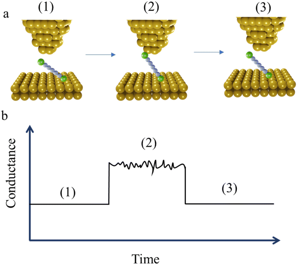 | ||
| Fig. 4 (a) Schematic illustration of the steps involved in the STM-based I(t) or “blinking” method: (1) tunnelling through the gap, (2) formation of molecular junction; and (3) junction breakdown. (b) Schematic of typical I(t) trace, annotated to indicate the steps of molecular junction formation and cleavage shown in (a). | ||
Unlike implementations of the STM-BJ technique that are drawn from the methods described by Tao,9 but in common with the I(s) approach, the STM tip in the I(t) measurements does not crash into the surface of the substrate, and therefore preserves the surface of the substrate and the shape of the STM tip shape. Although it is not possible to precisely control the morphology of the tip, electrochemical etching allows atomically sharp surface features to be created. Furthermore, it is possible to choose the area of the substrate with certain roughness by prior STM imaging; together, this allows a degree of information concerning relationships between junction formation and conductance on the underlying junction contact morphology.57 In many respects the I(t) and I(s) measurement methods have more in common than either have with STM-BJ and other break-junction methods that commence with formation and cleavage of an electrode–electrode contact. Nevertheless, it has been demonstrated that all three methods (I(t), I(s), STM-BJ) give the same (or similar) molecular conductance for a given molecular structure.52,58
2.2 Mechanically controllable break junction (MCBJ)
A typical mechanically controllable break junction (MCBJ) setup consists of flexible substrate, typically a phosphor bronze, supporting a thin metal wire fixed to the substrate at both ends and freely suspended over a pit, pore, trench or channel (Fig. 5). Prior to the measurements, the wire is lithographically notched or manually cut so that a thin bridge remains over the free region of space.59 When assembled, two stationary rods holds the sides of substrate down while a pushing rod presses from underneath, curving the middle of substrate up. This results in breaking the wire and by controlling the position of the pushing rod, a precise opening or closing of the gap between the electrodes can be achieved (Fig. 5). Target molecules can be assembled on the electrodes in advance (by drop-casting) or can be added as a solution of the target molecule in a liquid cell on top of the substrate/electrode assembly.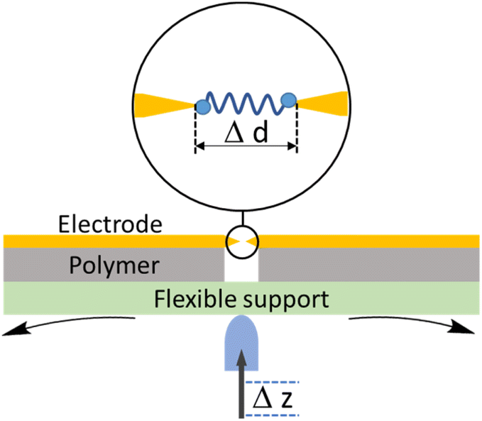 | ||
| Fig. 5 Schematic illustration of the MCBJ experimental assembly. | ||
The MCBJ technique has some advantages compared to the STM-BJ method. For example, whilst both methods allow the gap between two electrodes to be precisely controlled, the low displacement ratio between the horizontal movement of the nanogap and the vertical movement of the pushing rod coupled with the high mechanical stability of the MCBJ apparatus allows more ready calibration of the electrode gap. Secondly, the MCBJ configuration can be modified, providing the opportunity for on-chip device fabrication, such as lithographically fabricated MCBJ samples using sandwich structures with back gating.60 In addition, the more open device geometry in MCBJ permits combination of the electrical measurements in the MCBJ with gap-mode Raman spectroscopy to allow in situ monitoring of the molecule within the junction simultaneously with the charge transport measurements.61 These relative advantages of MCBJ are offset by the more diverse and readily exchanged tip and substrate electrodes in STM-based methods and the ready access to heterojunctions in which electrode materials of different type are used as the source and drain. Also, the STM-BJ exploits substrates with large, flat surfaces which allows many different regions to be explored, while MCBJ uses two electrodes with narrow tips that can make it harder to obtain the desired coverage of molecules in an experiment.51,62,63
2.3 Conducting probe atomic force microscope break junction (CP-AFM-BJ/AFM-BJ)
The conducting probe atomic force microscope break junction (CP-AFM-BJ or AFM-BJ) technique uses a conductive probe with a cantilever to combine the laser system inherent to an AFM with a current measurement circuit, allowing both the force and conductance signals to be measured simultaneously during break junction experiment (Fig. 6). The typical AFM-BJ method can be described in the following sequence of steps that begin when the conductive AFM tip is brought towards the sample in tapping mode until it comes into contact with the target molecule. As the tip is retracted from the surface, it pulls and stretches the molecule. While retraction of the tip takes place at a constant velocity, conductance and the interaction force between the tip and the molecule is measured until the junction breaks. The data obtained from the AFM-BJ experiment can provide information relating to the forces experienced on tip contact and junction cleavage,64,65 configuration66–69 and conformation70 of the molecule in the junction, and other aspects of the molecule–electrode interface.71–73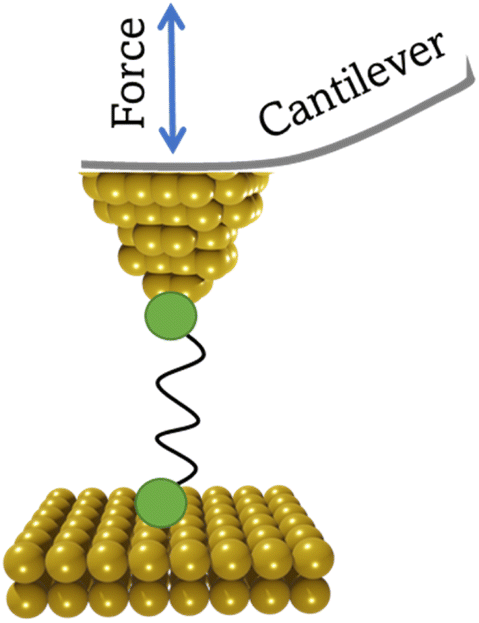 | ||
| Fig. 6 Schematic illustration of the AFM-BJ technique. | ||
3. Analysis of current–distance traces
Regardless of the method of collection, general characteristics of current vs. distance (Δz) plots can be highlighted; in addition, given the direct relationship between conductance and current, similar features are observed in conductance vs. distance plots, and closely related features are also observable from plots of conductance made on log(G) or log(G/G0) scales. Beyond the most probable conductance values that can be extracted from I vs. Δz traces, additional information is contained within the plateau length, which, as noted above, can be extracted from the break-off distance and corrected by the snap-back distance to give an indication of the ‘length’ of the junction (i.e. absolute electrode separation at point of junction rupture). Furthermore, in addition to the plateau ‘length’, the shape of the conductance plateau reflects the different physical and chemical processes taking place in the junction during measurements (Fig. 7). Together, the length and shape of the plateau in the I (or G) vs. Δz plots provide a more complete description of the behaviour of the junction. Analysis of these features can therefore be critical to not only the deeper understanding of single-molecule chemistry, but also the application of single-molecule junctions as tools in chemical reaction mechanism elucidation and sensing.74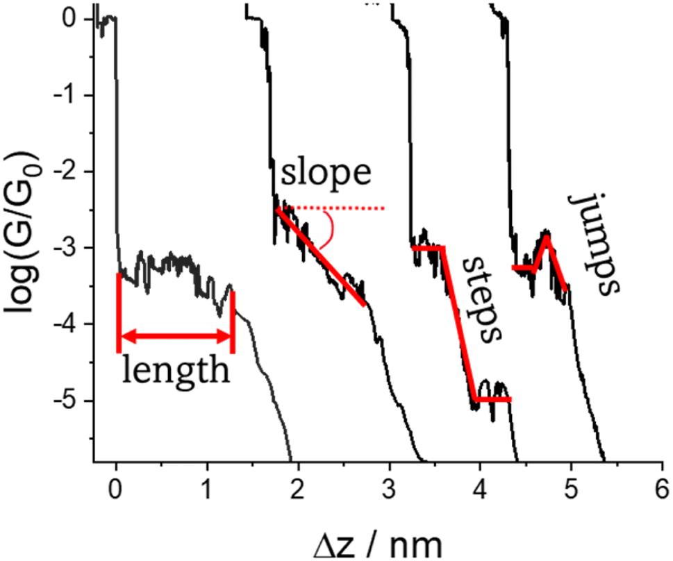 | ||
| Fig. 7 Conductance–distance traces (displaced along the Δz axis for clarity) with examples of different features (length, slope, steps and jumps) that characterise junction formation and evolution events. | ||
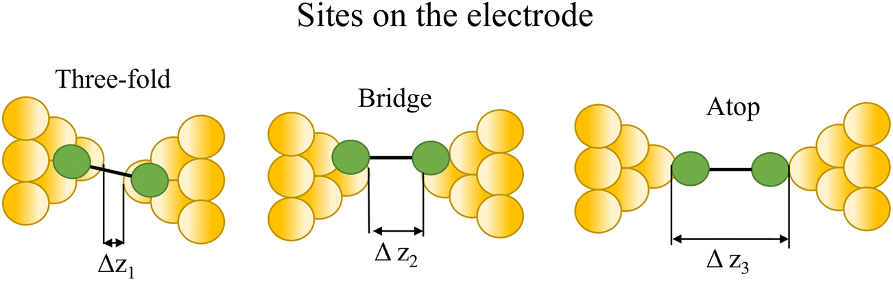
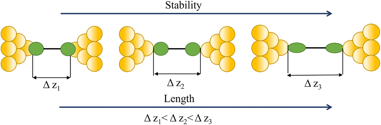
At the macroscopic level, the events involved in the formation, evolution and breaking of a single molecule junction are reproducible. However, at the molecular level, there are many highly stochastic events that lead to the significant junction-to-junction variation. On an aggregate level, these variations from many thousands of individual measurements manifest in the width of the conductance peaks observed in histograms. However, the individual traces each contain data arising from the evolution one specific junction. In the STM-BJ and MCBJ approaches, for example, the process of forming the molecular junction depends on factors including shape of the filament and the final shape of the fresh electrodes,75,76 the initial binding position of the analyte on the electrodes (e.g. at three-fold,17 bridge,18 or atop19 sites on the metal surface), and binding configuration or site of initial electrode–molecule contact (end-to-end or in-backbone contact77) (Table 1).
| Factor | Example | Ref. |
|---|---|---|
| Factors affecting length of a plateau in a current or conductance trace | ||
| Binding site |
|
17–19 |
|
77–80 | |
| Stability of a junction |
|
65, 66 and 81–83 |
| Pulling gold atoms from an electrode |
|
64, 67, 70 and 84–87 |
| Coupling and polymerization |
|
88 and 89 |
|
23, 87 and 90 | |
| Supramolecular interactions |
|
91, 92, 101–103 and 93–100 |
| Isomerization |
|
104–107 |
| Tautomerization |
|
43 and 108 |
![[thin space (1/6-em)]](https://www.rsc.org/images/entities/char_2009.gif) |
||
| Factors affecting shape of a plateau in a current or conductance trace | ||
| Slope | ||
| Stability of the junction |
|
82 and 109 |
| Stability of supramolecular interaction |
|
110 |
| Steric properties of the side group |
|
23 |
|
||
| Steps | ||
| Change in a contact angle |
|
47, 111 and 112 |
| Change in a contact group |
|
113 |
| Host–guest interaction |
|
114 |
|
||
| Spikes/jumps | ||
| Mechanical rupture of a bond in a molecule |
|
115 and 116 |
| Change in binding configuration |
|
117 |
| Force-induced resonant enhancement |
|
118 |
| Supramolecular radical junction formation |
|
119 |
| Quantum interference |
|
69 |
The detailed mechanism of how each junction forms and evolves after the initial cleavage of the Au–Au atomic contact and creation of the molecular junction as the electrodes further retract usually remains unclear, although some general situations can be envisaged,11 including the extrusion of gold atoms from the electrode surface(s) or the molecule sliding across the electrode between binding sites. Processes leading to a change in molecular conformation or geometry, such as isomerization reactions, the formation or dissociation of molecular dimers, assemblies or aggregates through supramolecular interactions also are evident as changes in junction conductance and appear as features in the conductance traces. Chemical reactions within the junction, such as inter-molecular (cross-)coupling or polymerization reactions can also lead to transitions between conductance states, often linked to changes in junction length. In addition, photochemical, acid–base, coordination or redox reactions can lead to well-defined switching phenomena. As a result of these different events that can take place during the stretching of the junction, the ‘plateau’ in the conductance vs. distance trace is rarely flat (i.e. a plateau that corresponds to a constant current or conductance value vs. distance) but rather may gently slope, feature one or more step wise drops in conductance, or exhibit sudden jumps to higher or lower conductance.41
3.1 Factors affecting plateau length (or ‘why is the junction shorter or longer than the molecular length?’)
In an idealised model, the plateau length corrected for snap-back (z*) would correlate with the length of the fully extended molecule in the junction, allowing for the geometry of the molecule relative to the surface normal imposed by the contact group chemistry. However, the plateau length varies significantly from trace to trace and depends on a range of different factors including binding configurations,120–123 stability,81 and other processes during molecular junction evolution,112 and which often occur in combination. The correlation of current flowing through the junction or conductance with changes in junction length therefore contains information relating to changes in the molecular geometry within the junction during measurement.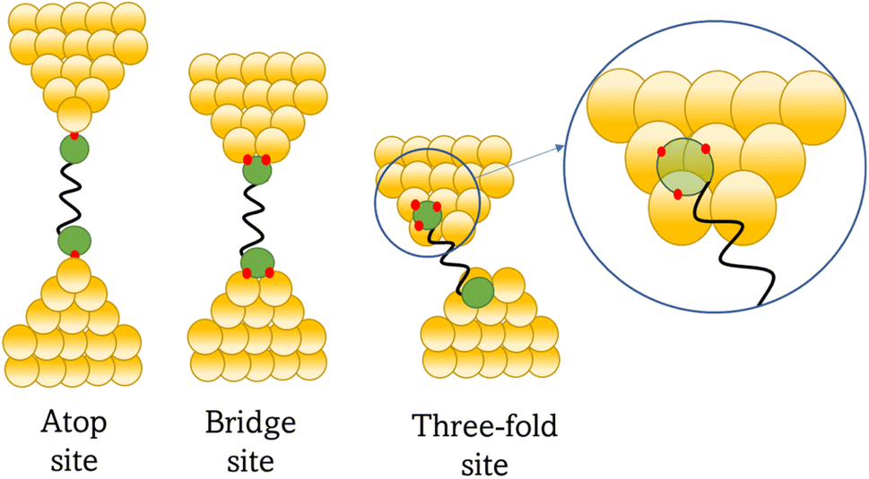 | ||
| Fig. 8 Examples of the different positions of an anchor atom to surface feaures of an electrodes from left to right: atop site, bridge site, and three-fold site. | ||
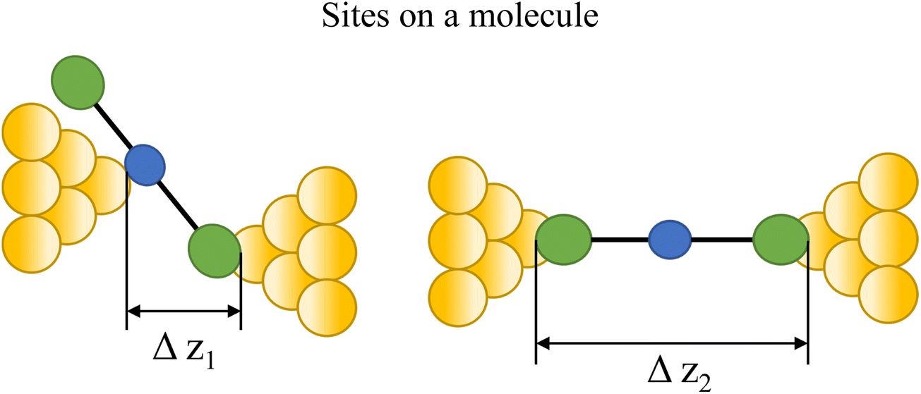
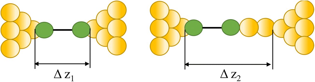
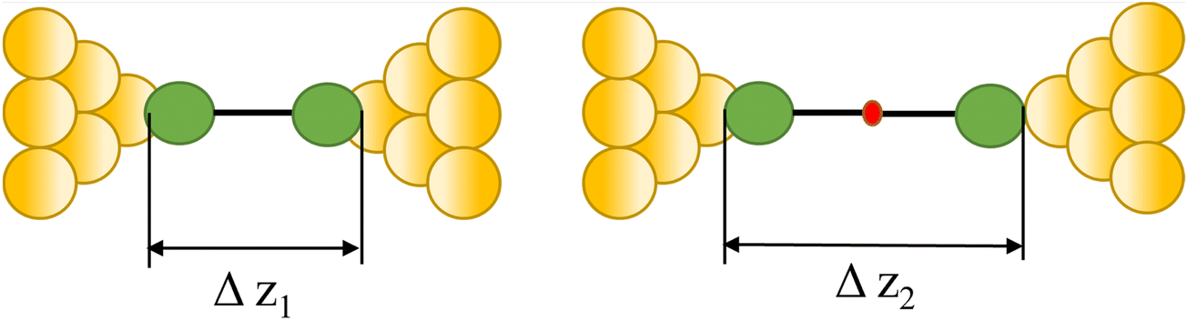
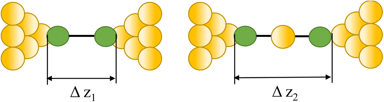
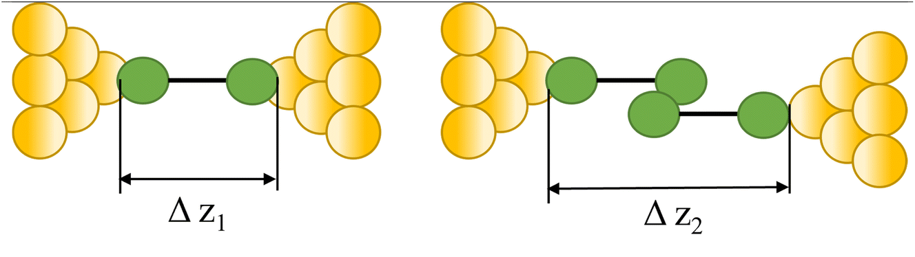
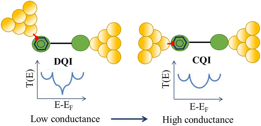
Beyond the behaviour of a single binding group located at the remote ends of molecules anchoring at either electrode interface, the electrodes may also contact to additional functional groups positioned to create multipodal terminal anchors.124–126 For example, platform and tower configurations have been proposed to account for variations in junction lengths formed from asymmetrically contacted tripodal molecules (Fig. 9a and b).78 The platform configuration illustrates a more general point that the presence of additional functional groups capable of promoting electrode contact inserted along or within the molecular backbone, whether intended for that purpose of not,127 can lead to a range of molecular junction geometries. The interplay of these additional contacting points with and across the electrode surface will naturally cause further variety in the number, conductance values and lengths of observable conductance plateaus.78,79 For example, pyrimidine moieties contained within the general backbone structure of common oligophenyleneethynylene (OPE) style molecular wires have been found to give rise to two conductance features arising from plateaus with different lengths as a result of two configurations of binding molecule: one, the conventional end-to-end configuration which gives plateau lengths corrected for snap-back approaching the end-to-end molecular length; and a second, much shorter junction in which one of the electrodes contacts directly to the pyrimidine ring (Fig. 9c and d).77
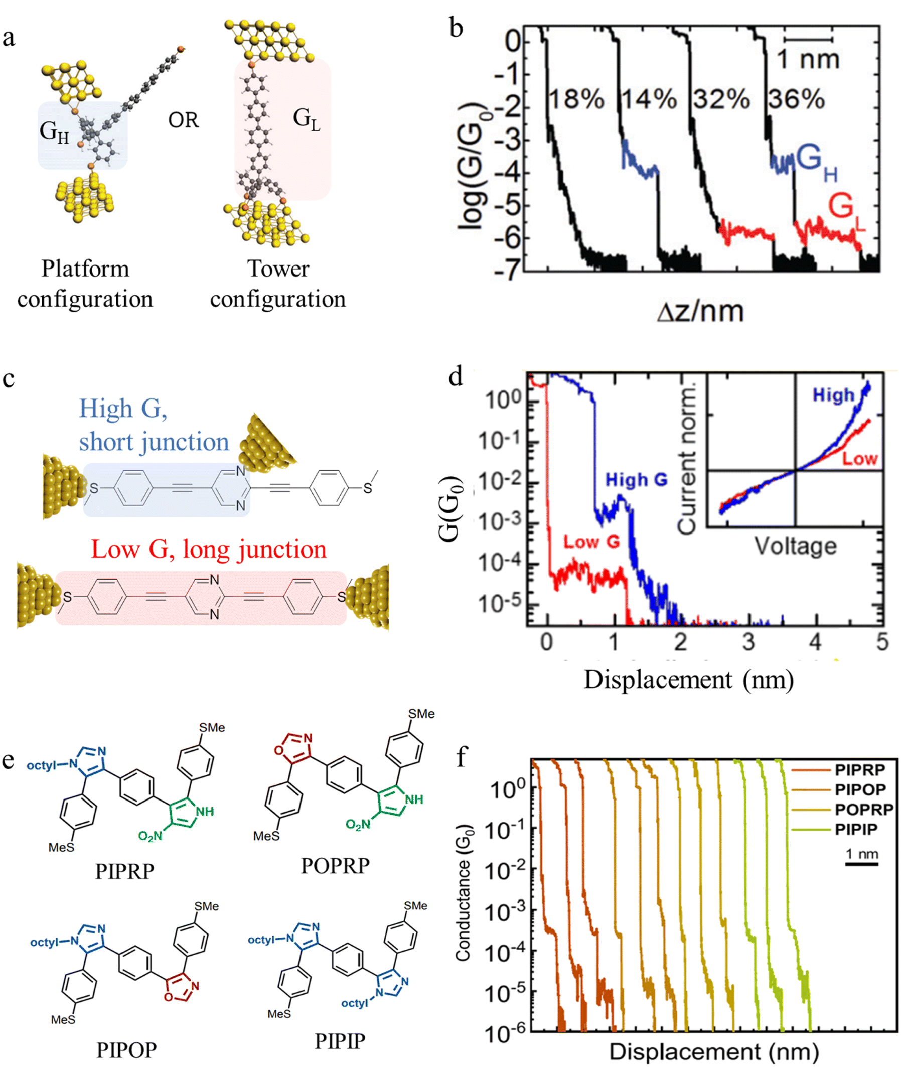 | ||
| Fig. 9 (a) Examples of platform and tower configurations of p-oligophenylene molecular wires with tripodal anchors; (b) examples of conductance traces with high conductance (GH) and low conductance (GL) features assigned to the different binding modes illustrated in (a); (c) schematic representation of end-to-end contacted and in-backbone contacted heterocyclic (pyrimidine) OPE type molecules; (d) examples of conductance traces with short, high-conductance junctions (blue) arising from in-backbone contacts and longer, lower conductance junctions (red) arising from end-to-end contacts of pyrimidine derivatives illustrated in (c); (e) conjugated oligomers with alternating heterocycle backbones; (f) characteristic single-molecule conductance traces of sequence-defined pentamers from (e) exhibiting multiple conductance peaks (applied bias 0.25 V). For these oligomers, two well-spaced conductance peaks are observed: short plateaus with high conductance (10−3.5G0); and long plateaus of lower conductance (10−4–10−5G0). Figures adapted with permission from ref. 77–79. Copyright 2019, Royal Society of Chemistry, Copyright 2015, American Chemical Society, Copyright 2020, American Chemical Society. | ||
In a similar vein, studies of oligomers in which the position of three distinct heterocycles (oxazole, imidazole, and nitro-substituted pyrrole) were precisely controlled along an otherwise comparable π-conjugated backbone gave rise to multiple conductance states which varied for dimers, trimers, pentamers, and a heptamer.79 It was found that the high conductance states arise from charge transport through short in-backbone linkage of imidazole or nitro-substituted pyrrole, whereas the low conductance state arises from the long charge transport path through terminal methyl sulfide anchor groups (Fig. 9e and f). The robust contacts to the backbone that give rise to the higher conductance plateaus were only formed in structures where the alignment of the in-backbone anchor (nitro-substituted pyrrole) and the terminal anchor (methyl thioether) was nearly linear.
In-backbone contacted junctions have also been observed under strong applied electric fields.80 For an amino-terminated aniline trimer (ATAT, Fig. 10a), as the bias across the junction was increased, leading to a larger electric field across the molecule in the junction, a higher conductance feature appeared. The 2D histograms constructed from these data demonstrated that the lengths of the conductance clouds collected under applied biases of 0.09 V and 0.45 V were 0.95 nm, and associated with a low conductance region, and 0.46 nm in a high conductance region, respectively (Fig. 10b and c). It was suggested that the electric field could induce the imine nitrogen atoms to bind as in-backbone linkers, giving rise to shorter, and hence more conductive, junctions.80 This bias-dependent binding would in turn permit switching between multiple conductance states under influence of the applied electric field.
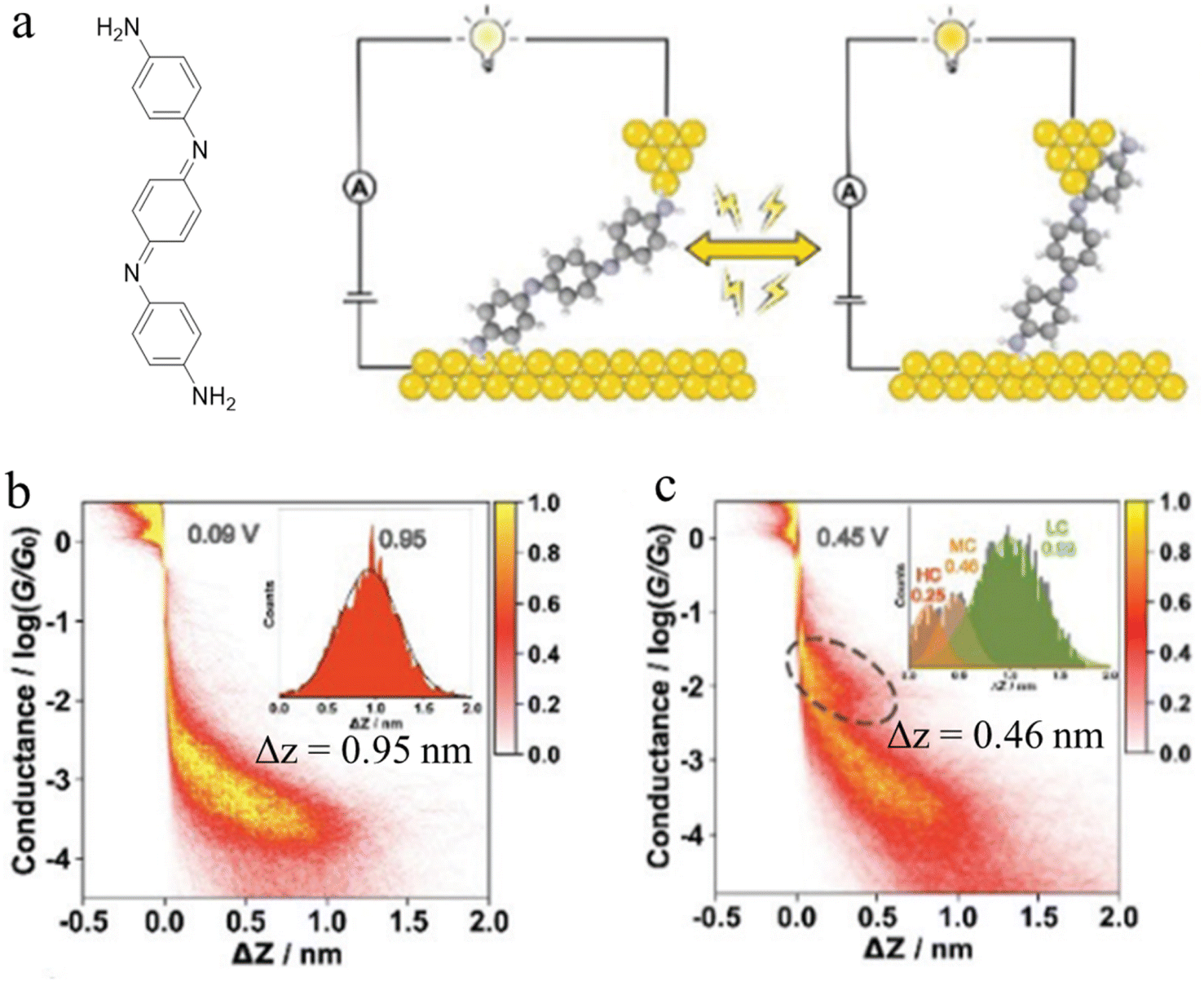 | ||
| Fig. 10 (a) Schematic of the single-molecule junction of ATAT under different applied bias; 2D conductance histograms of ATAT under (b) 0.09 V and (c) 0.45 V bias voltage, with the inset image of the corresponding displacement distributions of the plateaus. Figures adapted with permission from ref. 80. Copyright 2021, Royal Society of Chemistry. | ||


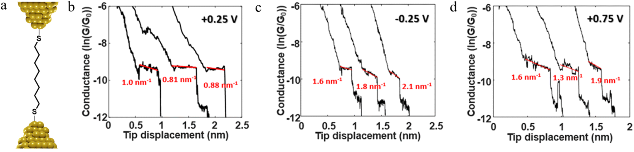
The stability of a molecular junction, and hence the length of the conductance plateaus, has also been shown to be influenced by the applied electric field of a gate electrode.81–83 For example, the mechanical stability and electromechanical properties of gold–octanedithiol(ate)–gold molecular junctions are sensitive to redox events due to the oxidation of Au at high potentials and the reduction of the S–Au bond at low potentials (Fig. 11a and b).82 The reduction of the S–Au bond involves an associated protonation reaction that together convert the thiolate S–Au contact to a weaker thiol SH–Au interaction and ultimately leads to desorption of the resulting alkanethiols from the Au electrode.129 It was found that the longest length of plateau was formed from octanedithiol with a gate potential of +0.25 V, and plateau lengths decreased with either increasing the gate potential toward the oxidation potential of Au (+0.75 V), or a decrease of the potential towards the reduction potential of the S–Au molecule–electrode contact (−0.25 V) (Fig. 11c–e).82 A similar pattern of behaviour is known for un-gated molecular junctions formed from diamine and dicarboxylic-acid-terminated alkanes, with increasing junction bias leading to weaker binding of the molecules to gold electrodes.81
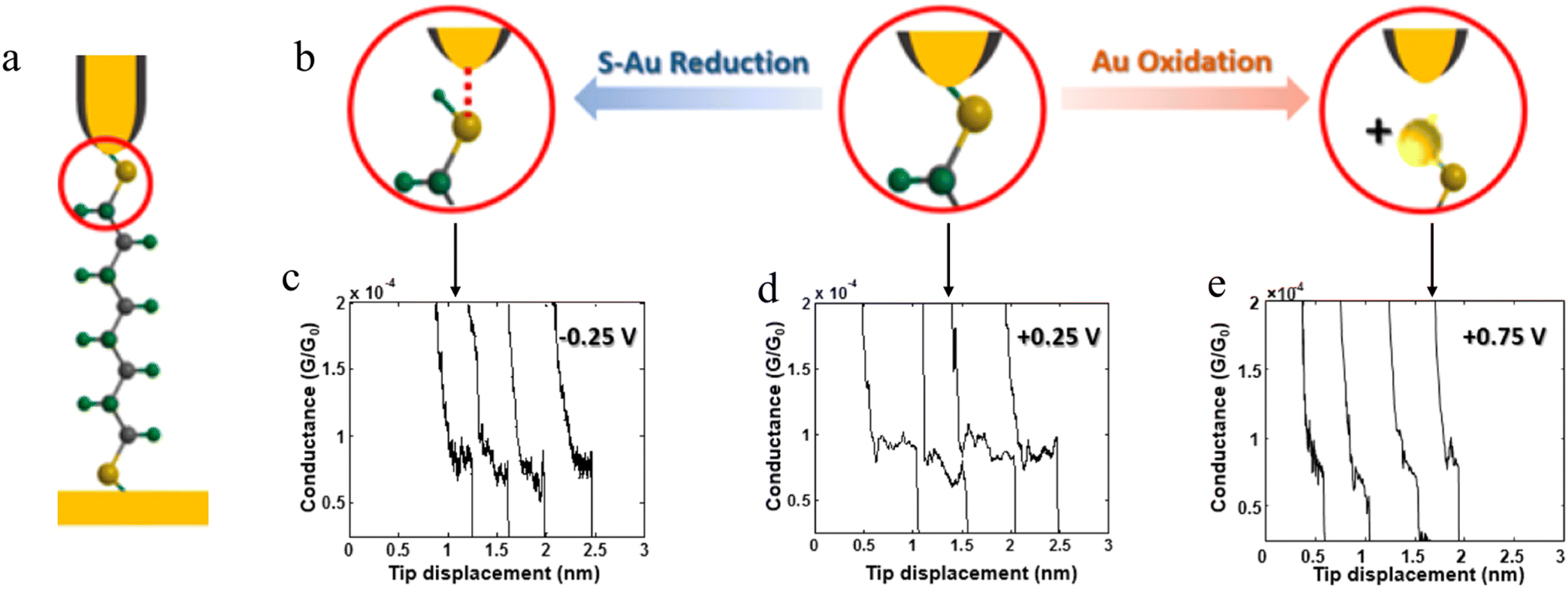 | ||
| Fig. 11 (a) Schematic of an octanedithiol(ate) junction; (b) molecule–electrode contact at different gate electrode potentials; conductance traces at (c) −0.25, (d) +0.25, and (e) +0.75 V. Figures adapted with permission from ref. 82. Copyright 2018, American Chemical Society. | ||
Experimental and theoretical studies reveal that solvent interactions within the junction can also influence the molecule–electrode binding energy and hence junction stability as the electrodes are withdrawn. For example, an analysis of the conductance features in single molecule junctions formed from 2,6-bis(((4-acetylthio)phenyl)ethynyl) anthracene in a triiodobenzene/1,2,4-trichlorobenzene (TIB/TCB) mixed solvent system revealed plateaus with three distinct lengths (ca. 0.46 nm, ca. 0.64 nm and ca. 0.92 nm; Fig. 12a–c). The longest plateaus (ca. 0.92 nm) originate from junctions that cleave by rupture of the Au–S bond without any interaction with the solvent.130 The plateaus of intermediate length (ca. ≈0.64 nm) arise from junctions weakened by an interaction between metal atoms in the junction electrode and the TCB solvent via a Cl⋯Au interaction. This halogen–metal interaction decreases the Au–S bond energy from ca. 1.5 eV to ca. 1.0 eV and increases the probability of breaking process of the Au–S bond. The shortest plateaus (ca. 0.46 nm) are also due to solvent–metal atom induced weakening of the molecule–electrode contact, by now from I⋯Au interactions with the triiodobenzene component of the solvent mix which further decreases the bond energy to ≈0.5 eV.130
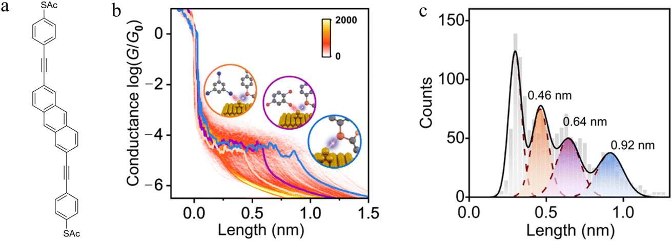 | ||
| Fig. 12 (a) Structure of 2,6-bis(((4-acetylthio)phenyl)ethynyl) anthracene with acetyl-protected thiol(ate) (–SAc) terminal groups; (b) 2D conductance–displacement histograms for the junctions in TIB/TCB. The orange/purple/blue lines are three typical single traces with different plateau lengths. Insets: schematic illustration of Au–S bonds in different cases: interaction with I (orange), with Cl (purple), and without I or Cl (blue); (c) conductance plateau lengths for junctions in TIB/TCB: the blue colour represents the parent junctions, the purple colour represents the case with Cl⋯Au interactions, the orange colour represents the case with I⋯Au interactions. Figures adapted with permission from ref. 130. Copyright 2023, Springer Nature. | ||
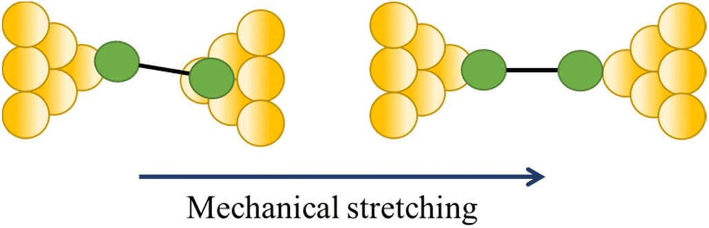
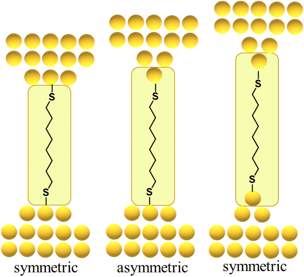
By way of one such example, the force required to break the Au–S contact in a molecular junction formed from a single octanedithiol molecule attached (as the thiolate) to gold electrodes is similar to the force required to rupture a Au–Au bond in an atomic gold chain. This suggests that the dithiolate molecule can pull Au atoms from the electrodes when a sufficient external force is applied, a conclusion supported by molecular dynamics simulations that indicate a thiolate molecule can pull gold atoms off a stepped surface.64,67,70,85 In related work with similar molecular junctions, it was demonstrated that as the electrodes are pulled apart, it becomes energetically favourable for Au atoms migrate to positions between the electrode surface and the sulfur atom contact, with junction structures alternating between what might be loosely termed ‘symmetric’ and ‘asymmetric’ configurations reflecting the idealised scenario as one or both electrode surfaces restructure (Fig. 13).84 Examples of extrusion of Au atoms from electrodes within junctions featuring molecules anchored by C–Au86 or imidazole N–Au bonds87 have also been demonstrated.
 | ||
| Fig. 13 Schematic of gold atom extrusion processes within an exemplary gold|octanedithiolate|gold junction during pulling of the electrodes. | ||
![[double bond, length as m-dash]](https://www.rsc.org/images/entities/char_e001.gif) N–) bridge (Fig. 14b).
N–) bridge (Fig. 14b).
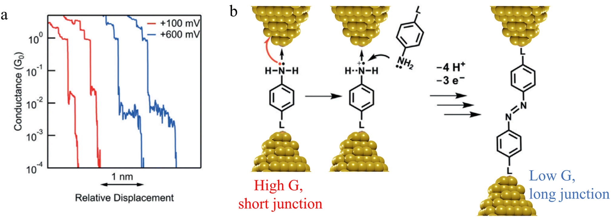 | ||
| Fig. 14 (a) Conductance traces of 4-mercaptoaniline measured at bias of +100 mV (red) and +600 mV (blue); (b) mechanism of a formation of azobenzene derivatives via electrooxidation of anilines in single-molecule junctions where L is aurophilic linker group (thiol, thiomethyl, alkynyl, or pyridyl). Figures adapted with permission from ref. 88. Copyright 2019, Wiley-VCH Verlag GmbH & Co. KGaA. | ||
In situ polymerisation of molecules trapped within a molecular junction can also occur as a result of transmetalation (from, e.g. tin,131 gold,132 or boron88), desilylation reactions,133 and dehydrogenative bond formation,134 all leading to C–C homocoupling reactions. An electric potential-promoted oxidative coupling reaction of organoboron compounds, such as aryl boronic acids, has also been reported and monitored with the STM-BJ technique.89 It was found that the transmetalation process of 4-(methylthio)phenyl boronic acid was controlled by the applied potential (Fig. 15a). At low-bias voltage, the first step of the transmetalation process occurred, giving rise to an intermediate Au|C-contacted junction and an associated short plateau and conductance cloud in the high conductance region (Fig. 15b). When higher-bias voltages were applied, a second cycle of the transmetalation process was induced, leading to close proximity of aryl species within the junction and the corresponding coupled products resulting in a longer conductance plateau in the low conductance region (Fig. 15c).89
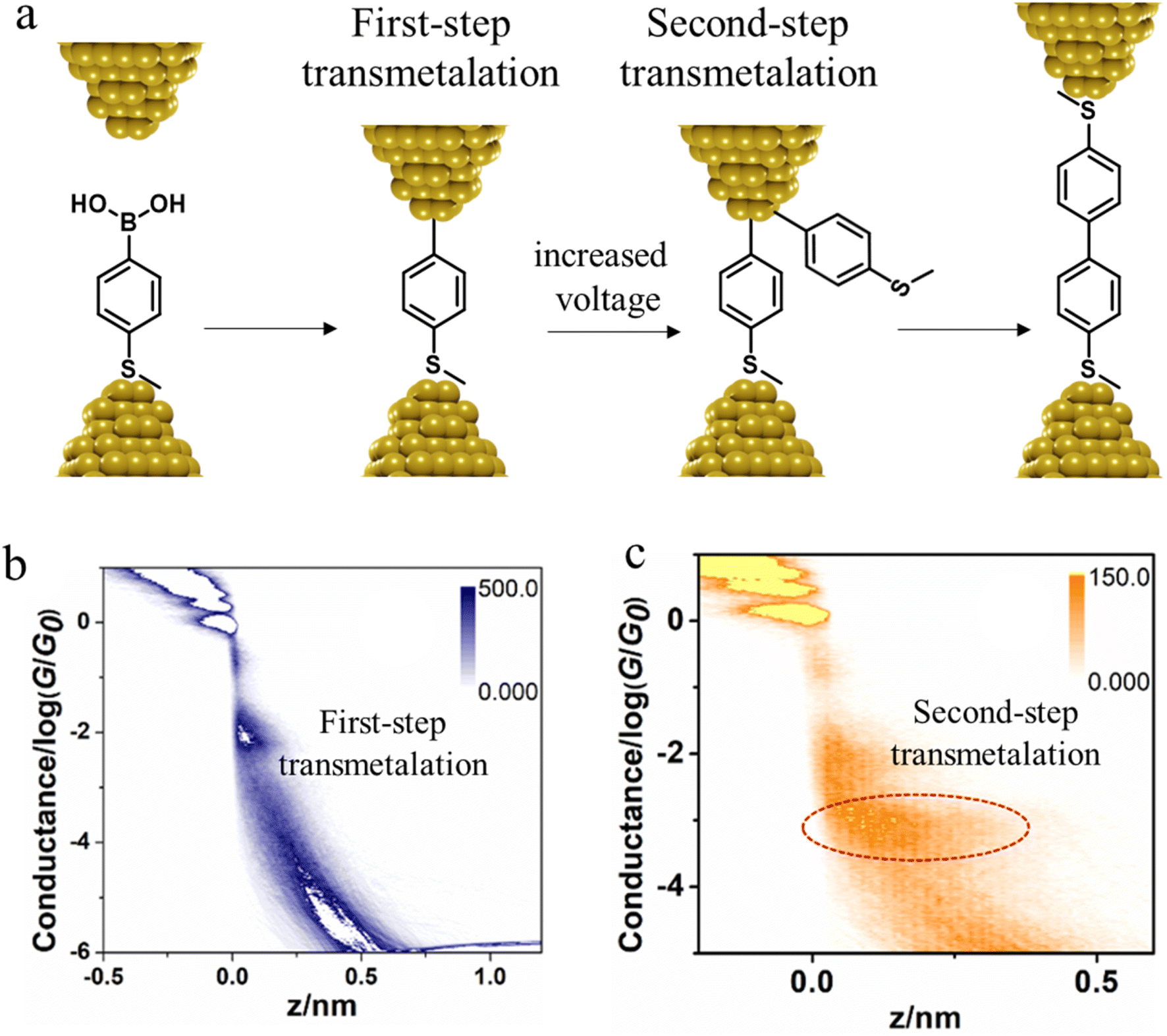 | ||
| Fig. 15 (a) A schematic of the electric potential-promoted oxidative coupling reaction of 4-(methylthio)phenyl boronic acid; (b) 2D conductance histogram of 4-(methylthio)phenyl boronic acid under 100 mV; (c) 2D conductance histogram of 4-(methylthio)phenyl boronic acid under 200 mV. Figures adapted with permission from ref. 89. Copyright 2022, Chinese Chemical Society. | ||
Beyond oligomerisation processes within the junction, as noted above, processes involving metal-atom extraction from the electrode and rearrangement of the electrode surface structures, extrusion of wire-like filaments and other dynamic processes of the metal electrodes can also strongly influence the dynamic processes of junction evolution and the appearance of current or conductance–distance traces. In addition to the gold surface case noted above, molecules contacted to metal electrodes by anchor groups with large binding energies that compete with the metal–metal bond energies are able to promote not only the rearrangement of the metal surface (vide supra) but also the complete extraction of metal atoms from the electrodes during extension of the junction. These undercoordinated atoms then provide further sites at which to incorporate additional molecules from solution and build metal-linked oligomers. In one such example, a sequence of long molecular junctions with break-off distances greatly exceeding molecular length were observed to be formed from 1,4-diisocyanobenzene in gold STM-BJs, strongly indicating the formation of molecular oligomers.23 Due to Coulomb repulsion between the terminal C atoms, one isocyano moiety cannot couple directly to another isocyano group. Therefore, the most probable path for oligomerization is the formation of an organometallic chain, where molecules couple through extruded gold atom(s) (Fig. 16a and b). The model provides a justification for the experimental traces being more than twice as long as the length of the molecule as the growing chain incorporates one or two gold atoms during the formation of each repeat unit. A similar process of organometallic chain formation within a junction was proposed to account for the observed junction lengths formed from imidazole molecules. Under basic conditions, the imidazole moieties bridge the electrodes in the deprotonated form through the nitrogen atoms, with several molecules able to bind in series mediated by gold atom bridges.90
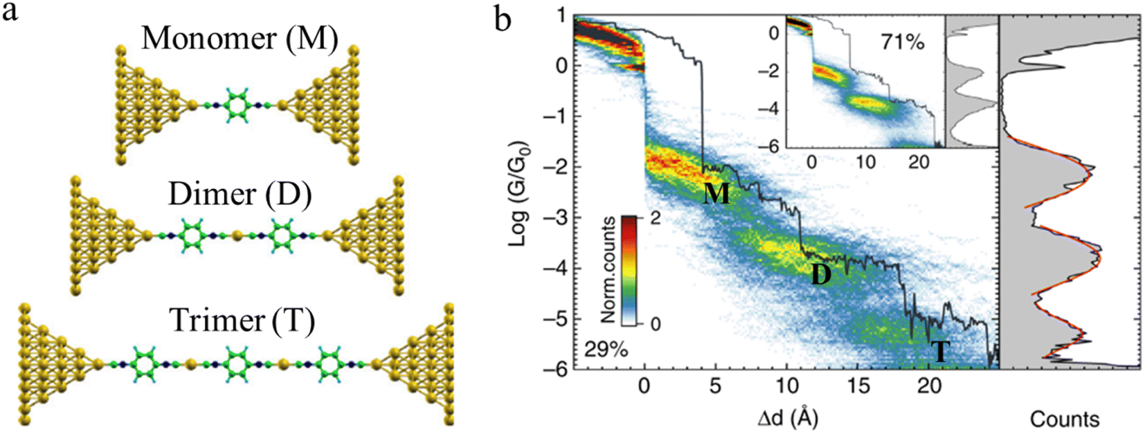 | ||
| Fig. 16 (a) Examples of junction geometries of 1,4-diisocyanobenzene containing one gold atom(s) in a junction: monomer (M), dimer (D), trimer (T); (b) Combined 2D–1D histogram with example conductance trace (29%) for 1,4-diisocyanobenzene. 2D–1D histogram for remaining traces (71%) is shown on the inset. Figures adapted with permission from ref. 23. Copyright 2019, Springer Nature. | ||
The observation of conductance plateaus longer than the molecular length of benzene dithiolates has led to proposals for the formation of metal–molecule oligomeric molecular wires.87 The standard model of the benzene dithiol junction (BDT) where a single BDT is sandwiched between two Au(111) surfaces (junction 1 in Fig. 17a) and three prototypical alternate junctions (2–4 in Fig. 17a) have been studied via DFT structure optimizations and molecular dynamics simulations. For junctions 2 and 4, which were designed to mimic the role of multiple benzene dithiolate molecules within the junction, additional molecules that do not span the electrode gap were modelled as methyl thiolate (SMe) to minimise computational cost. Junctions 1 and 3 show a mechanically stiff response, that sustain only 1–2 Å deviation from the minimum structure before breaking. Junction 2 demonstrated structural changes during elongation. The highest conductance of this junction found when the bond between the sulfur and the tip Au atom underneath (atom Au* in Fig. 17b) is stretched. When the S–Au* bond breaks, the conductance decreases steadily when the interaction between the tip atom Au** and the oxidized AuI atom in the RS-AuI-SR unit weakens. After that, a long molecular wire Au(tip)-SR-AuI-BDT-AuI-SR-Au(tip) is formed (Fig. 17b), which can be stretched significantly just by straightening the interatomic bonds while maintaining constant conductance. This is the key mechanism that produces the remarkable flexibility and increased length of junction 2.87 Depending on the experimental conditions, junctions that are close to the junction model 4 could also form, and providing a rationalisation for low conductance features.
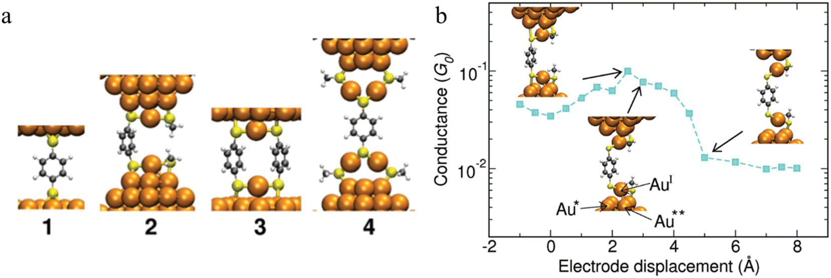 | ||
| Fig. 17 (a) Structures of the junctions 1–4 at mechanical equilibrium; (b) conductance of junction 2vs. the electrode displacement. The insets (from left to right): maximal strain of the S–Au* bond corresponding to the maximal conductance, breaking of the S–Au* bond, reflected in drop of the conductance, and subsequent elongation and breaking of the AuI–Au** bond. The conductance stays the same after the AuI–Au** bond is broken. Further stretching of RS-AuI-BDT-AuI-SR unit does not affect the conductance since the BDT is decoupled from the gold electrodes. Figures adapted with permission from ref. 87. Copyright 2010, American Chemical Society. | ||
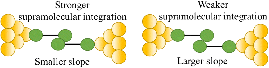
3.1.5.1 π–π stacking interactions. Whilst intramolecular charge transport is mediated by tunnelling processes through the molecular σ- or π-framework, intermolecular charge transfer typically operates by charge hopping between π–electron-rich regions of adjacent molecular structures. These π–electron-rich regions have a tendency to interact through non-covalent π–π and C–H⋯π motifs leading to supramolecular structures; such intermolecular interactions play an essential role in charge transport through organic materials and devices.93 Within a molecular junction, π–π stacking interactions between molecular fragments result in low conductance features with current plateaus longer than the length of the individual molecular fragments. The low conductance features from π-stacked junctions can be detected as independent features or as step-like continuations of a shorter, higher conductance plateau.91–93,100,101,103
Intermolecular π–π stacking interactions have been demonstrated in the junctions formed from monothiol-functionalised 1,4-bis(phenylethynyl)benzene. Despite the presence of only one strong anchor group, the junction formation probability was found to be similar to that of α,ω-dithiol analogues, with comparable statistical variation.91 As the junction is extended, the number of points of overlap between the π-systems, and hence the total strength of the intermolecular π–π forces, decrease. Consequently, π-stacked junctions are most commonly observed in junctions formed from molecules such as oligophenylene ethynylenes (OPE) with relatively long π-conjugated backbones capable of engaging many such π–π contacts. Since the junction is secured by these weaker, non-covalent interactions, the junction rupture force is significantly lower than that commonly associated with single-molecule junctions. These results imply that π-stacked junctions break by cleavage of the intermolecular π–π stacks rather than by cleavage of the molecule–electrode contacts. Nevertheless, π–π stacking can be used as the dominant associative force driving the formation of supramolecular bridges within few-molecule junctions.
Li et al. constructed a π-stacked thiophene dimer within an MCBJ platform to investigate the molecular-length-dependent intermolecular charge-transport properties (Fig. 18a).93 The molecular junctions were created by anchoring a thiophene molecule terminated at only one end by an –SMe group (denoted S-T1, 2-(4-(methylthio)phenyl)thiophene, Fig. 18a) to each atomically sharp gold electrode. By controlling the electrode separation to facilitate the π–π stacking interactions between two thiophene monomers two distinct plateaus with high conductance (H) and low conductance (L) features that appeared individually or together could be identified (Fig. 18b). The junction lengths of the H (0.68 ± 0.03 nm) and L (1.31 ± 0.02 nm) states were obtained from 2D histograms (Fig. 18c). The L conductance cloud is twice as long and more steeply sloped than the H conductance cloud, suggesting the formation of both a simple single molecule junction (responsible for the higher conductance features, Fig. 18a) and a single-stacked dimer of S-T1 which gives rise to the lower conductance junctions (Fig. 18a). In general, increasing the conjugated region improves the formation of the single-stacked junctions and facilitate transition from an intramolecular to an intermolecular path.101
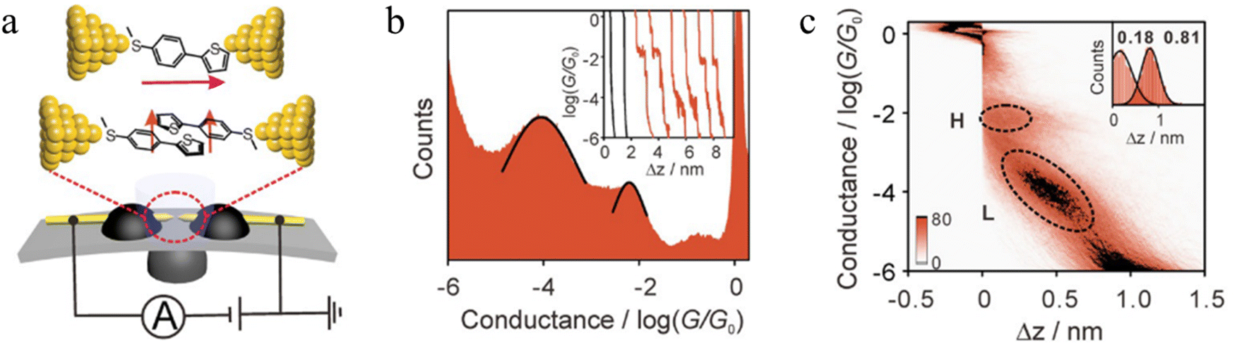 | ||
| Fig. 18 (a) Schematic of the MCBJ technique with a single-molecule S-T1 junction and a single-stacking S-T1 junction; (b) 1D histograms of S-T1. Inset; typical conductance–displacement traces of S-T1 where with example of black solvent traces; (c) 2D histogram of S-T1. Inset: relative stretching displacement histogram for H and L conductance features. Figures adapted with permission from ref. 93. Copyright 2019, Wiley-VCH Verlag GmbH & Co. KGaA. | ||
In some cases, π–π stacking interactions in a molecular junction are promoted by the increasing intensity of the electric field applied across the junction (i.e. electrode bias).92 In the absence of an electric field, the dihedral angles between adjacent benzene rings in terphenyl are 35°, a geometry that makes it quite difficult to form assemblies with strong π–π interactions and stable dimers (Fig. 19a). It has been demonstrated that the dihedral angles in an SMe-anchored terphenyl derivative decrease under an applied electric field, which makes the formation of π-stacked dimers more favourable (Fig. 19b). As the external field increases, the dihedral angles between the adjacent benzene rings in both conformations decrease to approximately 24°, which is more conducive to intermolecular π-stacking. Consequently, conductance features in low conductance region longer (by ca. 0.3 nm) than features in high conductance region have been observed (Fig. 19c).92
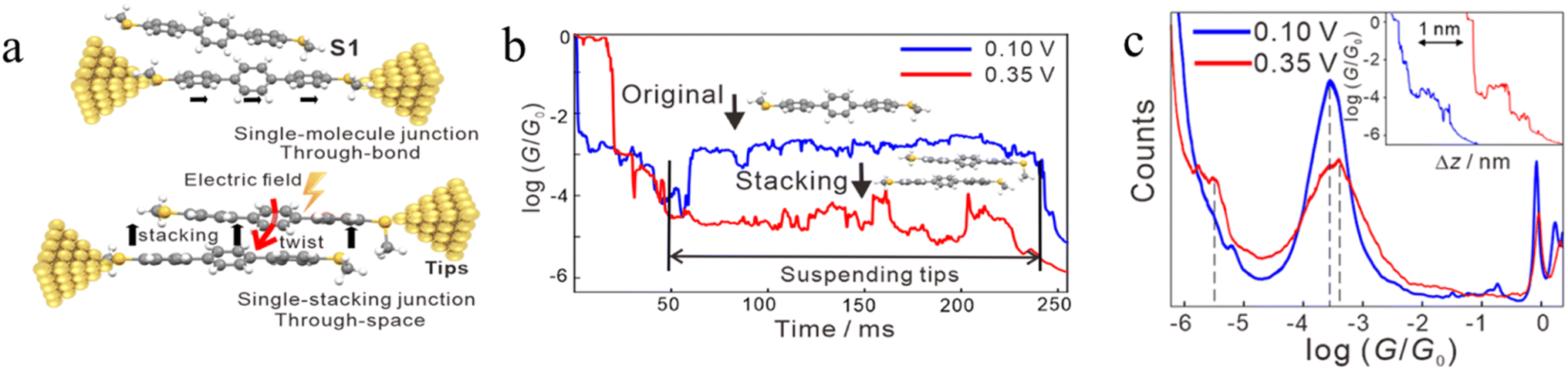 | ||
| Fig. 19 (a) Schematic of single-molecule junctions and single-stacking junctions of and SMe anchored terphenyl derivative; (b) two typical traces with the suspended retracting process under 0.10 (blue) and 0.35 V (red) for terphenyl; (c) 1D conductance histograms and typical conductance–displacement traces (inset) under 0.10 (blue) and 0.35 V (red); the black dashed line indicates the position of the conductance peak, and the inset is typical traces. Figures adapted with permission from ref. 92. Copyright 2020, American Chemical Society. | ||
3.1.5.2 σ–σ stacked supramolecular junctions. It has been demonstrated experimentally that a σ–σ stacking arrangement may also serve as the pathway of charge transport between two non-conjugated molecules, using mono-functionalised, 6-membered rings as a prototype system and comparing the π–π stacked junctions formed from benzenethiol and with the σ–σ stacked junctions formed from cyclohexanethiol (Fig. 20a).94 Conductance traces of benzenethiol junctions exhibited two different signals, in high (GH) and low (GL) conductance regions (Fig. 20b). These different conductance states (GH: 10−3.1G0 and GL: 10−4.4G0) with different length (GH: 0.68 nm and GL: 0.89 nm) have been attributed to the different stacking configurations of two neighbouring benzenethiol molecules within the π–π stacked benzenethiol junction. Importantly, cyclohexanethiol also exhibits different conductance states in the conductance traces (Fig. 20c).
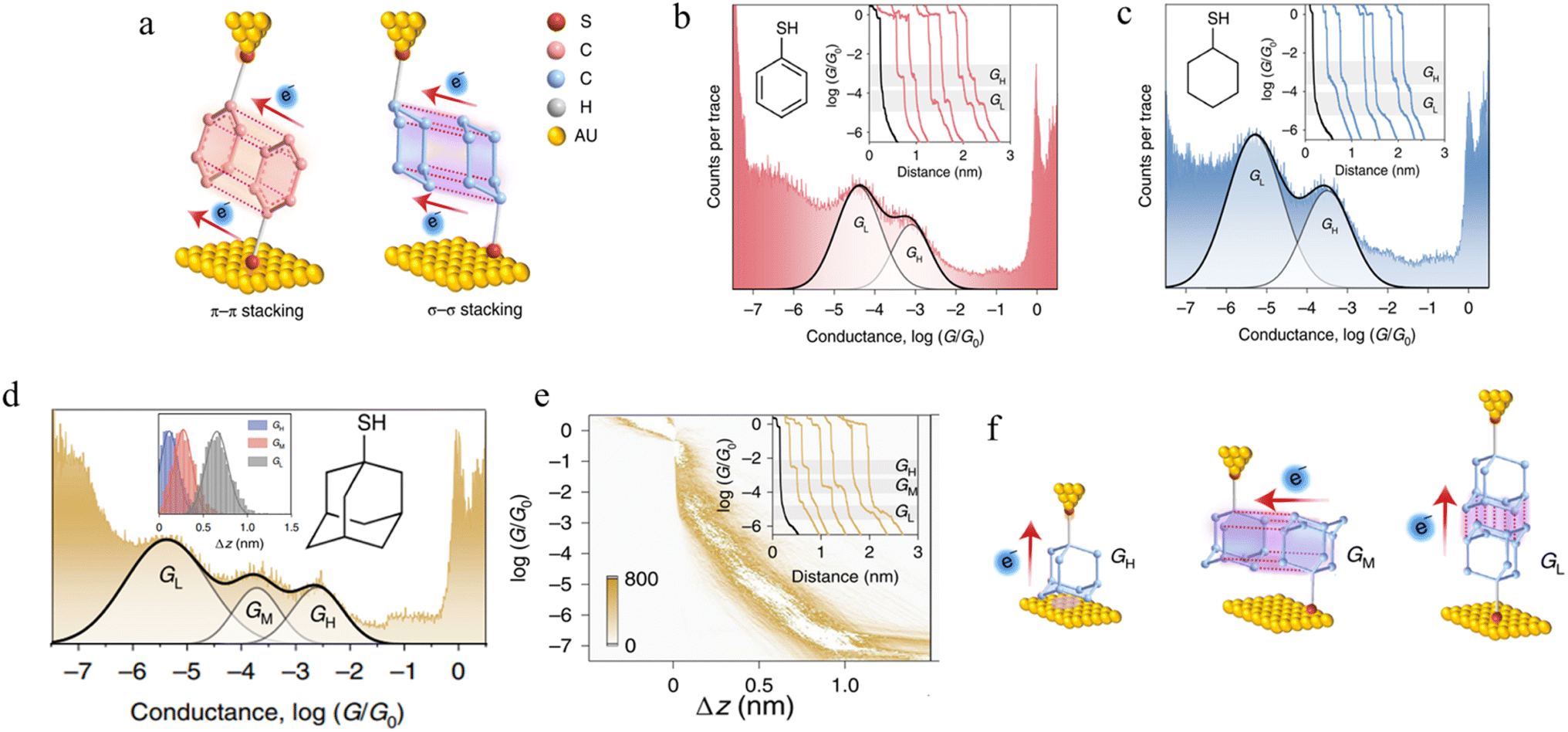 | ||
| Fig. 20 (a) Configuration schematics of π–π stacked molecular junctions of benzenethiol and σ–σ stacked cyclohexanethiol dimer junctions; (b) 1D conductance histograms of benzenethiol with example traces as inset; (c) 1D conductance histograms of cyclohexanethiol with example traces as inset. GH indicates a high-conductance feature and GL indicates a low-conductance feature. The black traces represent tunnelling decay in pure solvent without target molecules; (d) 1D conductance histograms of 1-adamantanethiol with the relative stretching distance distributions of molecular junctions as inset; (e) the 2D conductance–distance histograms of 1-adamantanethiol with individual conductance traces as inset; (f) configuration schematics of 1-adamantanethiol junctions formed between the gold electrode pair with GH, GM, and GL states. Figures adapted with permission from ref. 94. Copyright 2022, Springer Nature. | ||
It has been hypothesized that two cyclohexanethiol molecules are first connected to both electrodes by Au–S bonds; during the stretching cycles, the two molecules interact with each other, forming stacked molecular junctions give GH at 10−3.5G0 and GL at 10−5.3G0 with average length of the conductance features of 0.73 nm and 0.98 nm, respectively and which differ through the degrees of geometrically possible interaction. To verify the proposed σ–σ stacked molecular junctions, junctions formed from 1-adamantanethiol were also examined. The 1D and 2D histograms of 1-adamantanethiol exhibit three conductance states, denoted GH (10−2.6G0), GM (10−3.73G0) and GL (10−5.38G0) with plateau lengths of 0.62, 0.75, and 1.16 nm, respectively (Fig. 20d and e). The GH state was associated with a junction configuration where only one 1-adamantanethiol molecule is bound to the gold electrode and interacts with the substrate to form monomer junctions. The GM and GL stated were associated with the ‘side-to-side’ interaction configuration, the ‘head-to-head’ configuration (Fig. 20f).
Recently, calculations have revealed that the energy interaction in σ–σ stacking between two non-conjugated cyclohexane molecules is stronger compared to the π–π interaction between two benzene molecules,135,136 raising prospects for chemical design of a wider range of supramolecular structures in junctions than might have previously been envisioned.
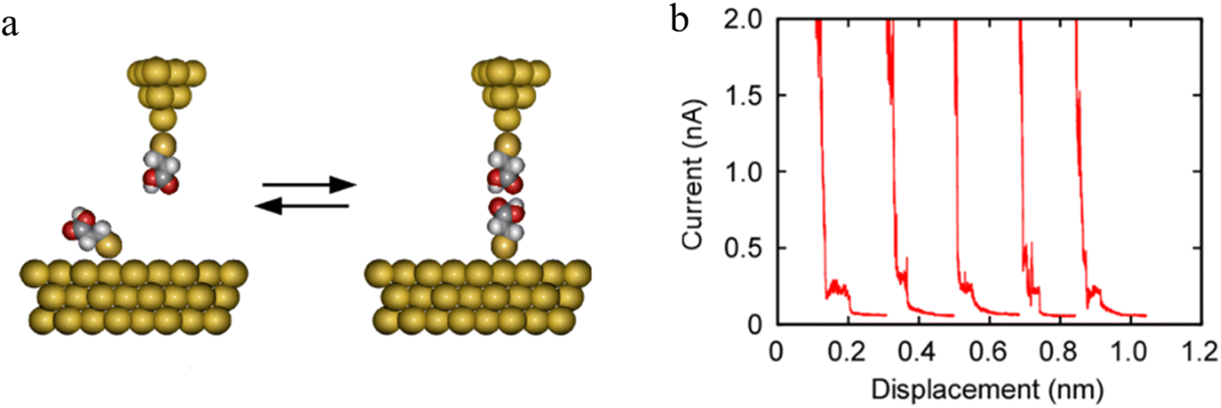
3.1.5.3 Hydrogen-bonded structures. Another explanation for the appearance of long plateaus during the processes of molecular junction evolution as a function of electrode separation is the formation of hydrogen-bonded oligomers.95–99,102 However, in general, junction formation probabilities for such H-bonded assemblies are relatively low (3–15%).95,97,137 This low formation probability may arise from: the stochastic molecular orientation on electrode surfaces which challenges the precise arrangement of H-bond donor and acceptor necessary for the formation of directional H-bonds, especially at greater electrode distances; the low rupture force of H-bonds compared to anchoring groups causes H-bonded dimers to break during stretching of metallic filaments in break-junctions, preventing migration into nanogaps; and/or the strongly oriented electrical field along supramolecular junctions that affects fragment polarity and subsequently impacts the formation probability of H-bonded assemblies.
The formation of H-bonded molecules within a junction was clearly demonstrated in STM-BJ studies of HS(CH2)2COOH. The plateaus on representative conductance traces (Fig. 21b) have been ascribed to tunneling current through these H-bonded carboxylic-acid dimers.
 | ||
| Fig. 21 (a) Schematic of carboxylic acid dimer based molecular junctions; (b) representative current–distance plots measured using Au|S(CH2)2COOH tips over Au|S(CH2)2COOH-covered surfaces. Figures adapted with permission from ref. 95. Copyright 2020, American Chemical Society. | ||
A series of ureido pyrimidine-dione (UPy) derivatives, modified with different anchoring groups, were also studied for evidence of the electron transport properties of H-bonded assemblies in apolar solvent by the STM-BJ technique (Fig. 22a).97 In the absence of self-assembled dimers, the conductance–distance traces exhibit the typical exponential decay after the tip has moved apart from the substrate (black curves). In the presence of the anchor group functionalised ureido pyrimidine diones 1–3, although most of the traces the show exponential decay characteristic of simple through gap-tunnelling (blue curves), certain individual data sets exhibit pronounced plateaus (red curves), which suggests the formation dimeric molecular wires of molecules 1, bridged by the quadruple hydrogen bonds (Fig. 22b). The JFP of the most conductive dimers formed from UPy-1 was estimated to 14.7%, with a conductance value that approaches 10−3G0.
 | ||
| Fig. 22 (a) Illustration of a supramolecular junction bridged with quadruple hydrogen based on UPy molecules with different binding groups (thiol, pyridyl, and amino). This noncovalent interaction exhibits conductivity comparable to that of covalently conjugated molecular devices and can also be manipulated by the polarity of the solvent environment; (b) typical conductance–distance curves of UPy-1. Figures adapted with permission from ref. 97. Copyright 2016, WILEY-VCH Verlag GmbH & Co. KGaA. | ||
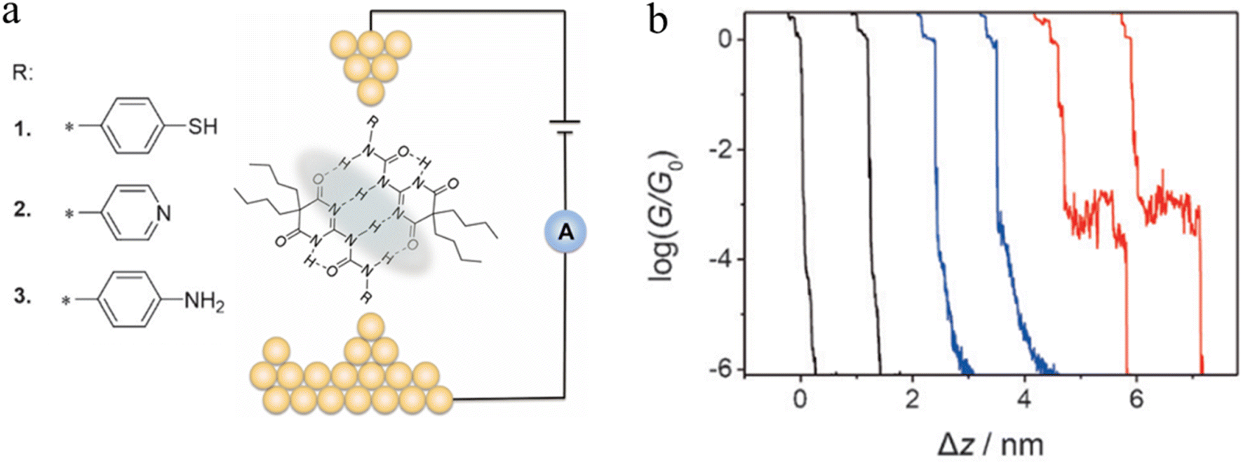
The single-molecule conductance of two supramolecular complexes formed through amidinium-carboxylate charge-assisted hydrogen bonds have also been studied, giving rise to junctions of length that exceed the dimensions of the individual components (Fig. 23a).102 The single-molecule conductance of compounds 4a and 5 have been determined to be log(G/G0) = −3.0 and −2.8 respectively (Fig. 23d and c). The 2D conductance histograms of mixtures of 4a and 5 feature two conductance regions (Fig. 23d). The higher conductance data cloud (log(G/G0) = −3.0) can be attributed to molecular junctions formed by either compound 4a or 5 with a plateau-length distribution (0.75 ± 0.02 nm) that also agrees with the dimensions of 4a or 5. On the other hand, the length of the lower conductance plateaus (ca. log(G/G0) = −6.0) is about double that of the individual components (1.52 ± 0.02 nm). This feature has been attributed to molecular junctions formed from the hydrogen-bonded assembly 4a·5. Similar events have been observed for mixtures of 4b and 5 consistent with the formation of complex 4b·5 (Fig. 23e).
 | ||
| Fig. 23 (a) Supramolecular H-bonded amidinium-carboxylate wires (4a·5 and 4b·5); 2D conductance histograms for (b) 4a, (c) 5, (d) complex 4a·5, (e) complex 4b·5. Figures adapted with permission from ref. 102. Copyright 2020, American Chemical Society. | ||
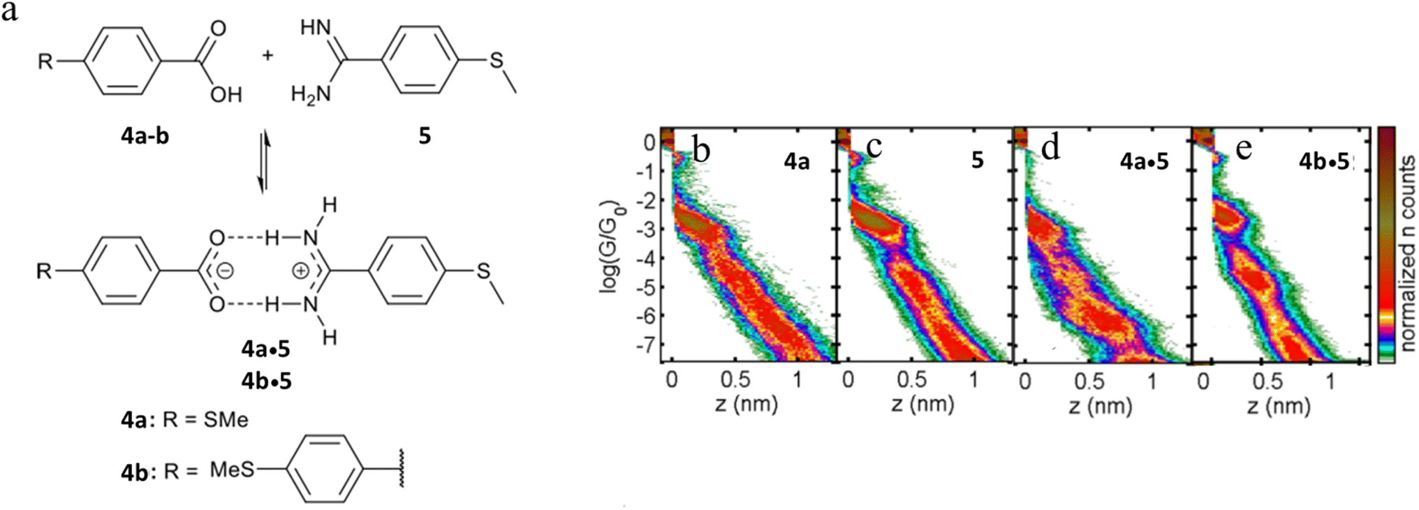
Beyond the use of chemically paired H-bond donors and acceptors, water molecules can be involved in H-bonding interactions within junctions, and provide unusual electrical transport properties and conductance plateaus with different length.98,99 The single-molecule conductance of 1H-imidazole (IMI) has been measured in a dry liquid medium resulting in multiple conductance features (Fig. 24a). The observation of long features that exceed the molecular length suggest formation of H-bonded assemblies (monomer to dimer to trimer) units as the junction is stretched (Fig. 24b). The molecular conductance of IMI in water results in a different conductive profile, and the multiple conductance signals observed in this case (Fig. 24c) are attributed to the formation of chains of alternating H-bonded imidazole and water molecules such as IMI–water–IMI (Fig. 24d).98
 | ||
| Fig. 24 Junction structures of (a) IMI trimer and (b) IMI–water–IMI complex optimised by DFT energy minimisation; (c) 2D conductance histograms of 1H-imidazole in an anhydrous environment and (d) and in water. Figures adapted with permission from ref. 98. Copyright 2020, Royal Society of Chemistry. | ||
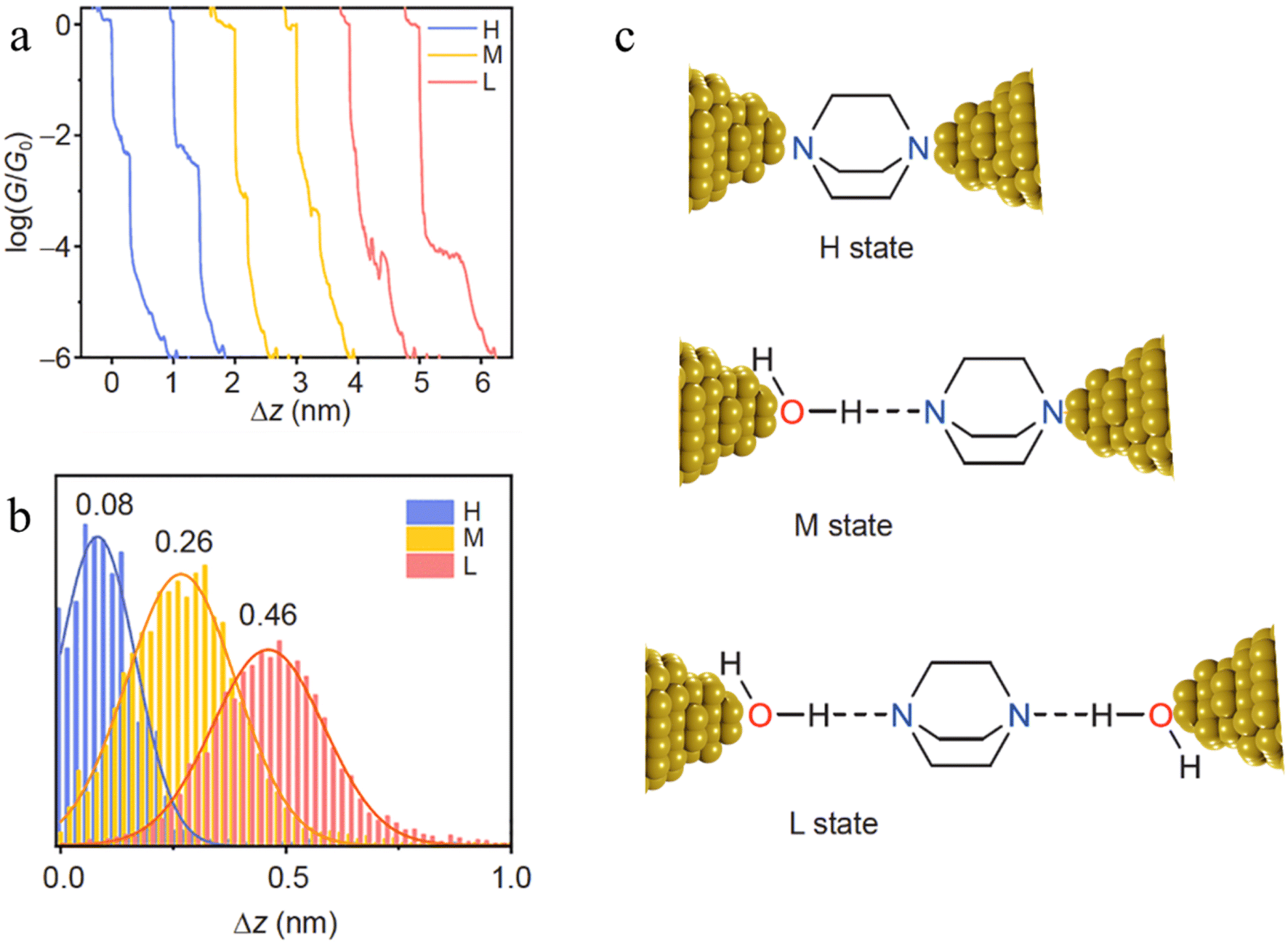
The inclusion of H-bonded water within molecular junctions has also been proposed to account for the single-molecule conductance vs. distance characteristics of 1,4-diazabicyclo[2.2.2]octane (DABCO) in 1,2,4-trichlorobenzene (TCB) solvent.99 The individual conductance traces determined from STM-BJ measurements demonstrated three types of plateaus with different lengths (Fig. 25a and b), with the various high (H, electrode|DABCO|electrode), medium (M, electrode|DABCO⋯H2O|electrode) and low (L, electrode|H2O⋯DABCO⋯H2O|electrode) conductance features attributed to inclusion no, one or two water molecules in the junction (Fig. 25c).99
 | ||
| Fig. 25 (a) Typical individual conductance–distance traces of the three conductance states of DABCO: H (blue), M (yellow), L (red); (b) the displacement distributions of the three states of DABCO. The most representative distance values are showing based on the Gaussian fitting; (c) the junction geometries of the three conductance states. The dash lines represent the hydrogen bonds. Figures adapted with permission from ref. 99. Copyright 2021, Science China Press and Springer-Verlag GmbH Germany. | ||
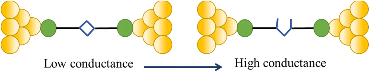
Molecules sensitive to photoisomerization processes have attracted attention in the general field of molecular electronics where they serve as switches and photomodulators.138 Molecular junctions formed from the E and Z isomers of 4,4-(ethene-1,2-diyl)dibenzoic acid are illustrated in Fig. 26a, and give a representation of the change in junction dimensions with molecular conformation. Isomerization of the conformers is achieved directly on the gold surface through photo-irradiation, and the STM-BJ is used to determine conductance before and after irradiation.104 The E isomer gives rise to lower conductance features with longer break-off distances (Fig. 26b), while the Z isomer is associated with relatively higher conductance junctions with shorter break-off distances (Fig. 26c).
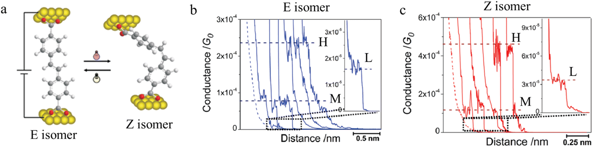 | ||
| Fig. 26 (a) Molecular structure of E and Z isomers of 4,4′-(ethene-1,2-diyl)dibenzoic acid in the junction; (b) conductance traces of E isomer; (c) conductance traces of Z isomer with high (H), medium (M), and low (L) conductance features. Figures adapted with permission from ref. 104. Copyright 2010, American Chemical Society. | ||
Beyond photochemical processes, electric fields have also been shown to direct and catalyse solution-phase reactions, and therefore applications of electric fields that lead to modification of the molecular scaffold within a junction can be identified as a potential input parameter to control junction behaviour. For example, cumulene derivatives, which consist of chains of carbon atoms bound together to give contiguous π-bonds, undergo cis-to-trans isomerisation reactions under an electric field (Fig. 27a). In single-molecule junction measurements, the conductance step length distribution as a function of time showed a clear transition from a predominantly shorter plateau (cis) at the start of the experiment, to longer plateaus attributed to the trans isomer formed in situ at the end of the experiment (Fig. 27b).106
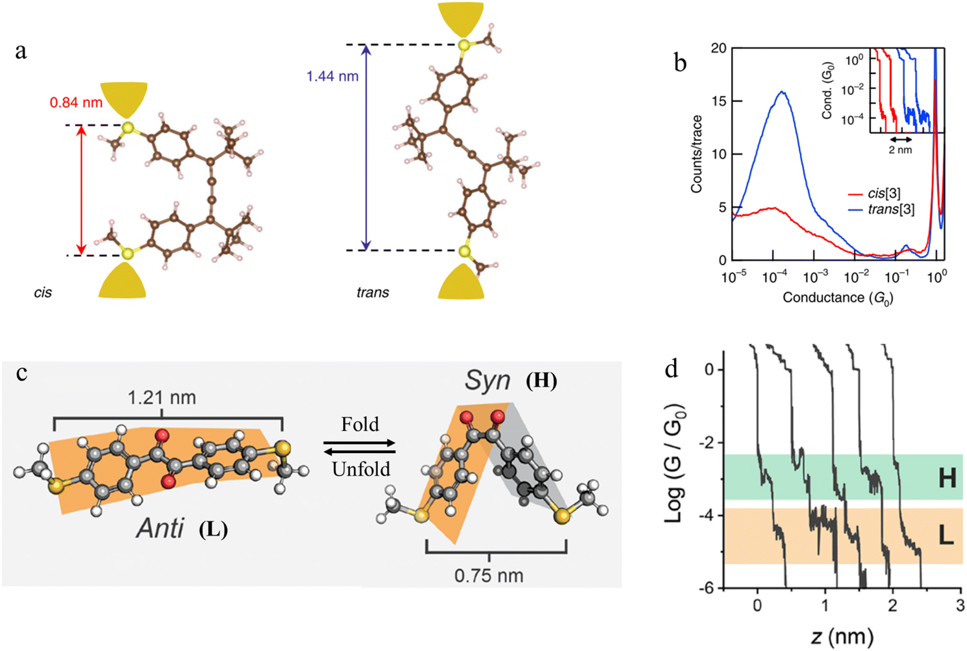 | ||
| Fig. 27 (a) Schematic of the single-molecule junctions with DFT-optimized structures of cis and trans isomers with S–S distance; (b) 1D histograms for cis (red) and trans (blue) isomers. Inset: example conductance vs. displacement traces of cis (red) and trans (blue); (c) three-dimensional structures of 1,2-bis(4-(methylthio)ethane)-1,2-dione in the anti (dihedral of 155°) and syn (dihedral of 23°) conformations with S–S length shown; (d) example of conductance traces of 1,2-bis(4-(methylthio)ethane)-1,2-dione. Figures adapted with permission from ref. 106 and 107. Copyright 2019, Springer Nature, Copyright 2020, American Chemical Society. | ||
Mechanical stimulus leading to confirmational change in a molecular scaffold can be achieved through the force imparted on a molecule by the junction electrodes. The syn and anti conformations of 1,2-bis(4-(methylthio)ethane)-1,2-dione differ in length (by ca. 0.4 nm) (Fig. 27c). The observed mechanosensitivity of 1,2-bis(4-(methylthio)ethane)-1,2-dione arises from an anti ⇌ syn conformational switch, as the molecule is folded along the flexible bond following junction compression or extension. Consequently, conductance traces collected from the syn isomer during junction extension show short conductance features in high conductance region (H) (syn configuration) and a step to a second, subsequent and longer feature in a low conductance region (L), attributed to the molecule being pulled into the anti configuration (Fig. 27d).107
 | ||
| Fig. 28 (a and b) Schematic representation of tautomerisem within an STM-BJ. The device is in the low-conductance keto state in which a σ-bridge connects the two contacts. After charge injection, the molecule within the junction transforms to the high-conductance state with a π-bridge. The cyan balls represent generic anchor groups, whilst the grey, red, and white balls represent carbon, oxygen, and hydrogen, respectively; (c) examples of conductance traces of 1,2-bis(4-(methylthio)phenyl)ethan-1-one measured at 0.1 and 0.6 V; 2D conductance histograms of compound 6 (d) at 0.1 V and (e) 0.6 V bias, with the stretching distances shown in the insets. Figures adapted with permission from ref. 43. Copyright 2023, Springer Nature. | ||
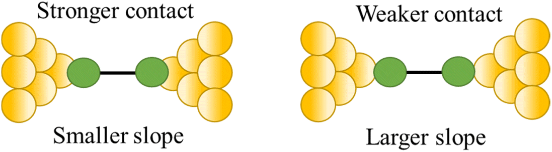
3.2 Factors affecting shape of the plateau
The various physical and chemical events that can occur within a molecular junction during the elongation (and compression) stages of a break junction mean that only rarely is the conductance plateau found at a single current value for the duration of the molecular contact. Rather more often, the conductance plateaus are sloped, or contain steps and sudden jumps which contain information pertaining to the dynamic physical and chemical processes taking place in the junction.| G = GCe−βL | (2) |
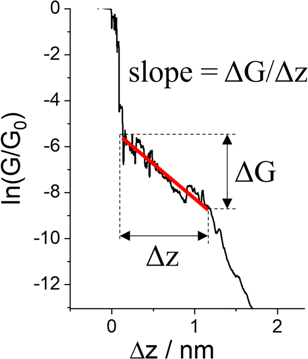 | ||
| Fig. 29 Conductance trace with plateau slope that determined as ΔG/Δs, where ΔG is conductance range where plateau appears, and Δz length of the plateau. | ||
For example, as discussed in Section 3.1.2 ‘Stability of the junction’, for junctions formed from octanedithiol and gold electrodes, the nature of the molecule–electrode contact varies due to reduction of the S–Au bond at low potentials and oxidation of the gold surface at higher potentials (Fig. 30a).82 The plateaus collected at +0.25 V gate potential are due to strong Au|SR (thiolate) contacts, and are relatively stable as a function of junction elongation, giving almost constant values of molecular conductance vs. electrode separation, and hence ‘flat’ plateaus. At lower (less positive) potentials, the Au–S bond is reduced and the weaker Au|S(H)R allows greater mobility of the molecule across the electrode surface and a greater slope to the conductance plateau. At higher (more positive) potentials, oxidation of the gold surface leads to AunO|SR junctions, and again weak molecule–electrode contacts, more mobile molecules within the junctions and increased slope to the conductance plateau (Fig. 30b–d). In addition to the break-off distance, the change in slope change provides important information indicating changes in the mechanical and electromechanical properties of the molecular junctions, with a greater slope in the plateau indicating mechanical instability of the junction.
 | ||
| Fig. 30 (a) Schematic of octanedithiol junction; example of conductance traces with linear fitting of the plateau at (b) +0.25 V, (c) −0.25 V, (d) +0.75 V illustrating the variation in electrical response vs. applied potential. Figures adapted with permission from ref. 82. Copyright 2018, American Chemical Society. | ||
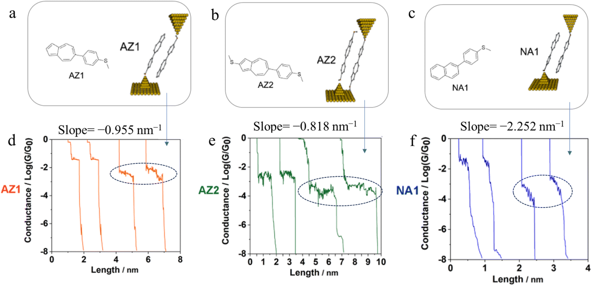
Further examples of the slope of a conductance plateau reporting the relative mechanical stability of a junction can also been seen in various π-stacked supramolecular junctions. It has been demonstrated that the π-stacked dimers formed by the polar, azulene-based compounds (4-(azulen-6-yl)phenyl)(methyl)sulfane (AZ1) and methyl(4-(2-(methylthio)azulen-6-yl)phenyl)sulfane (AZ2) (Fig. 31a and b) show higher electrical conductivity than those formed by the rather apolar, naphthalene-based methyl(4-(naphthalen-2-yl)phenyl)sulfane (NA1), reflecting the weaker π–π interactions in NA1 (Fig. 31c). In addition, the averaged plateau slope for NA1 (−2.252 nm−1) was significantly larger than those of AZ1 (−0.955 nm−1) and AZ2 (−0.818 nm−1), due to the lower mechanical stability of π–π interactions in the naphthalene-based dimers relative to the azulene-based structures (Fig. 31d–f).110
 | ||
| Fig. 31 Schematic of π-stacked dimer of (a) AZ1, (b) AZ2, and (c) NA1; representative individual conductance vs. distance traces of (d) AZ1, (e) AZ2, and (f) NA1 with value of slope for low conductance plateaus indicated by dotted circle. Figures adapted with permission from ref. 110. Copyright 2023, American Chemical Society. | ||
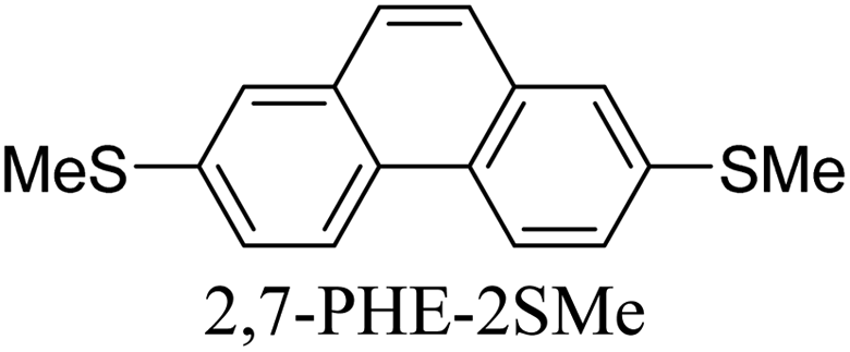
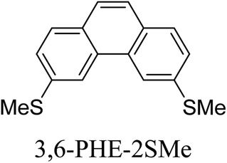
Junctions formed from phenanthrene derivatives with two methyl thioether anchors at different positions (PHE-2SMe) give rise to conductance plateaus that vary in slope (Table 3).109 The single-molecule junctions formed from 1,8-PHE-2SMe and 3,6-PHE-2SMe present the largest conductance plateau slopes, indicating that the molecular conductance drops rapidly with the length of the junction, arguably due to the restriction in range of stable binding configurations with surface gold adatoms.109 The conductance plateaus of 1,7-PHE-2SMe, 2,6-PHE-2SMe, and 1,6-PHE-2SMe show an intermediate slope, suggesting a more durable junction than 1,8-PHE-2SMe and 3,6-PHE-2SMe, but less stable than 2,7-PHE-2SMe.109 The absence of a clear correlation between calculated coupling strength (Γ) and conductance plateau slope for this series of compounds suggests that conductance plateau slope reflects the dynamics of the molecule within the junction during the electrode separation step.
| Structure | Slope/nm−1 | Γ/eV |
|---|---|---|
|
−2.18 | 1.50 × 10⁻³ |
|
−4.63 | 1.27 × 10⁻³ |
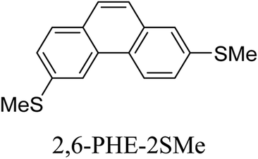
|
−3.64 | 3.09 × 10⁻⁴ |
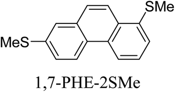
|
−3.75 | 1.29 × 10⁻⁴ |
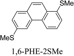
|
−3.75 | 8.65 × 10⁻⁵ |
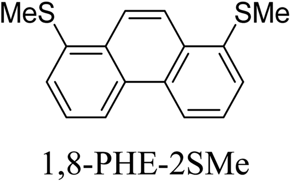
|
−4.40 | 2.35 × 10⁻⁵ |
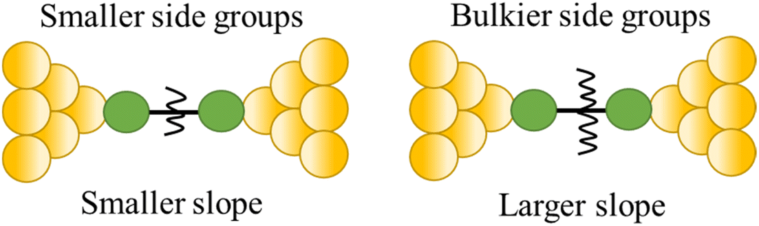
Break-junction experiments with various 1,4-diisocyanobenzenes featuring different side groups have demonstrated a dependence of the conductance plateau slope with both analyte concentration and steric properties of the side group (Fig. 32a).23 The 2D conductance histogram of the parent system displays a pronounced slope, which may be due to sliding of the molecule along the electrode surface as the junction electrode separation is increased. As the concentration of analyte increases, both the plateau width and slope of conductance cloud monotonously decrease (Fig. 32b). It has been proposed that the increased occurrence of π-stacked molecules (and decreasing number of free binding sites on the electrode surfaces) that may be expected with increasing analyte concentration reduces the number of mechanical degrees of freedom, limiting the variation in conductance vs. distance.23 In support of this proposal, for a fixed analyte concentration, bulky substituents which would be expected to reduce the formation of junctions featuring π–π interactions, and permit fewer stable binding geometries at the surface, lead to an increase in plateau slope (Fig. 32b).
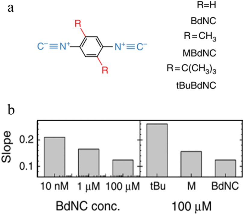 | ||
| Fig. 32 (a) Structures of isocyano compounds with different side groups; (b) dependence of plateau slope on different concentration and size of different side groups of the molecule. Figures adapted with permission from ref. 23. Copyright 2019, Springer Nature. | ||
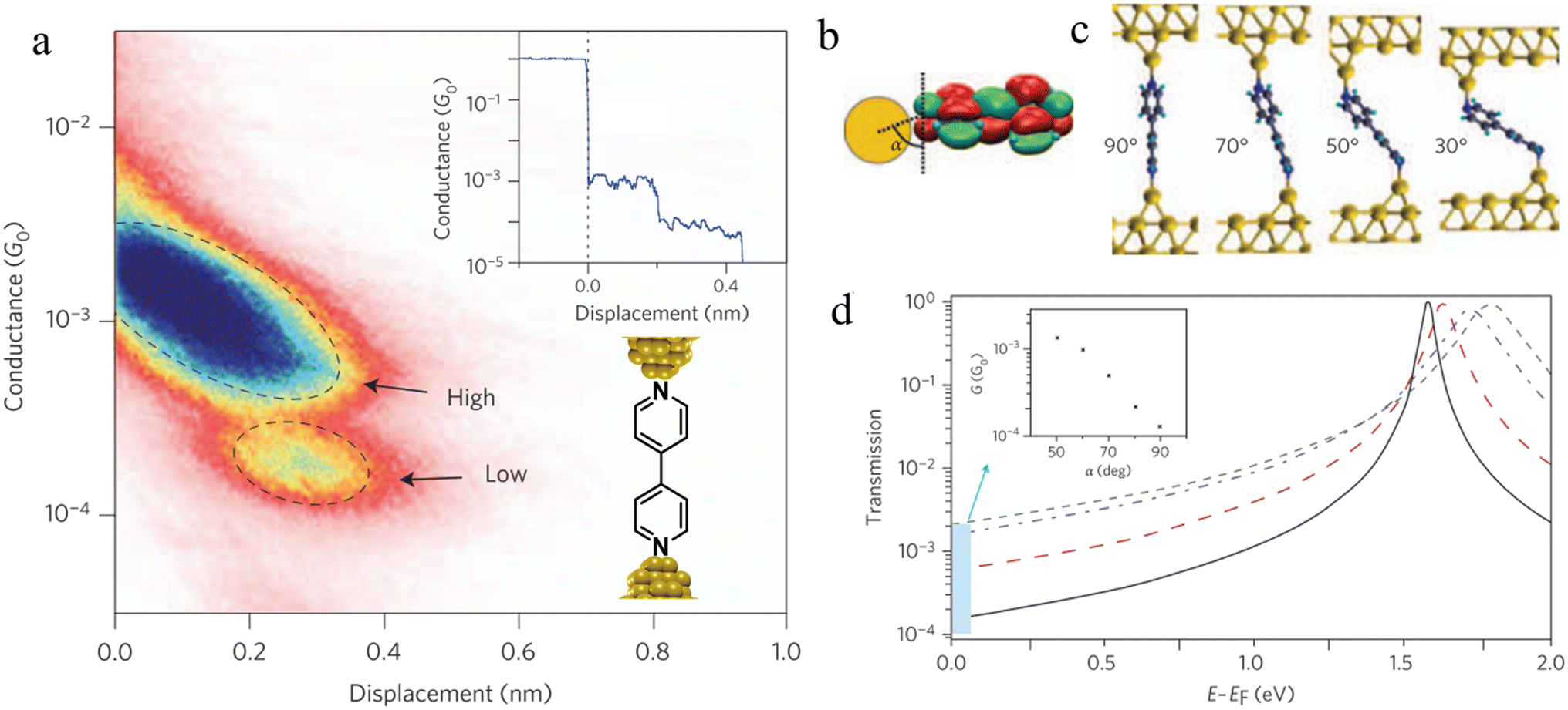 | ||
| Fig. 33 (a) 2D histogram with two conductance states – high and low. Inset: example of conductance trace with two steps; (b) schematic of the coupling between the gold–s-orbital (orange) with the bipyridine LUMO where α is the angle between the nitrogen–gold bond and the π*-system; (c) junction geometries of bipyridine bonded on each side to gold adatoms, with varying α; (d) self-energy corrected transmission functions plotted on a semi-logarithmic scale for the junctions: black solid line for α = 90°, red dashed line for α = 70°, blue dashed–dotted line for α = 50°, and green dotted line for α = 30°. The inset shows G decreasing with increasing α. Figures adapted with permission from ref. 111. Copyright 2009, Springer Nature. | ||
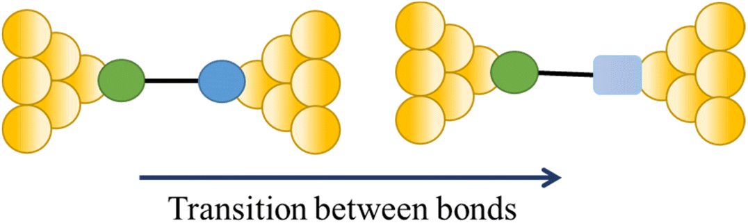
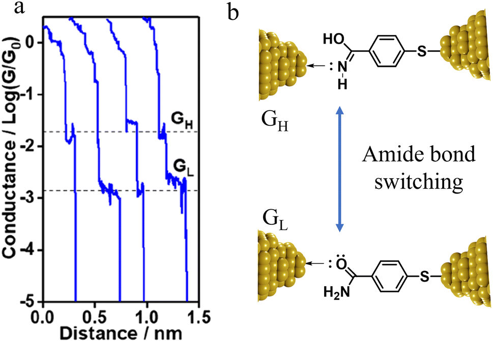
The compound 4-mercaptobenzamide (MBAm) also demonstrates bimodal charge transport behaviour through changes in contact at the amide linkage, which give rise to well-separated high (GH = 10−1.78G0) and low (GL = 10−2.72G0) conductance junctions (Fig. 34a).113 Density functional theory (DFT) simulations demonstrated that for shorter electrode separations, chelation of the amide promotes a proton transfer reaction. The resulting amide isomer-“iminol” product is stabilized by surrounding water molecules in the electrode gap, forming a robust Au–N linkage and increasing the coupling of the electrode with the molecular backbone (Fig. 34b). As the junction extends, the proton transfers back to reform an amide which binds in κ1(O)-fashion giving the lower conductance junction.
 | ||
| Fig. 34 (a) Conductance traces of MBAm in DI water; (b) transition between single and double bonds between N and C atoms in an amide. Figures adapted with permission from ref. 113. Copyright 2021, American Chemical Society. | ||
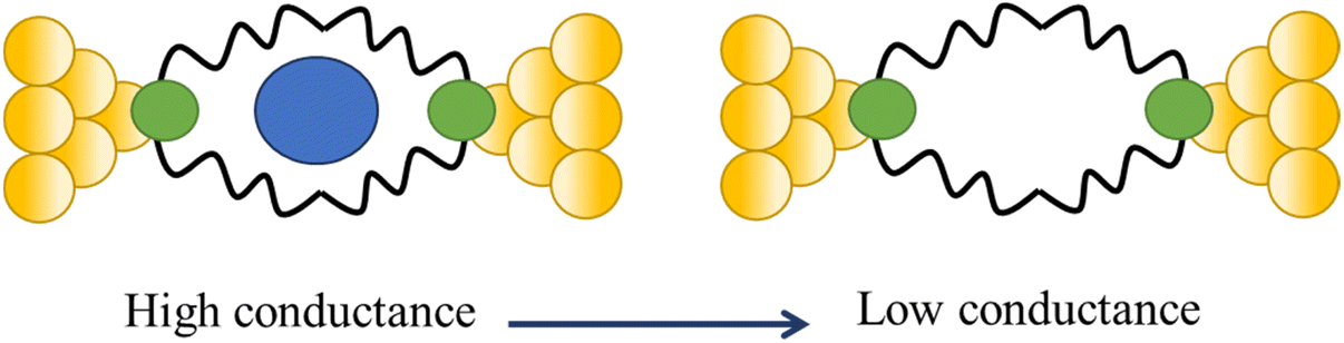
Tang and others have provided evidence of a large enhancement of conductance through the metallocycles (8–10) when a C60 guest is incorporated (Fig. 35a and b), with the inclusion of the guest leading to step-like conductance features in the resulting conductance–distance traces.114 Conductance plateau for the guest-free metallocycles 8, 9, and 10 were observed at 3.1, 1.4, and 0.6 × 10⁻⁵G0, respectively. In contrast, the conductance–distance traces of [8 + C60] and [9 + C60] display two conductance plateaus at different conductance levels (Fig. 35c). The low-conductance features similar those of the free metallocycles, while the higher-conductance features, including [8 + C60] at 2.8 × 10⁻⁴G0 and [9 + C60] at 1.7 × 10⁻⁴G0, suggested the formation of the host–guest complex with C60. In contrast, the junctions formed from solutions of 10 and C60 exhibit only one conductance plateau at 0.61 × 10⁻⁵G0, corresponding to the free metallocycle 10 suggesting that the host–guest complex does not form with this largest macrocycle.
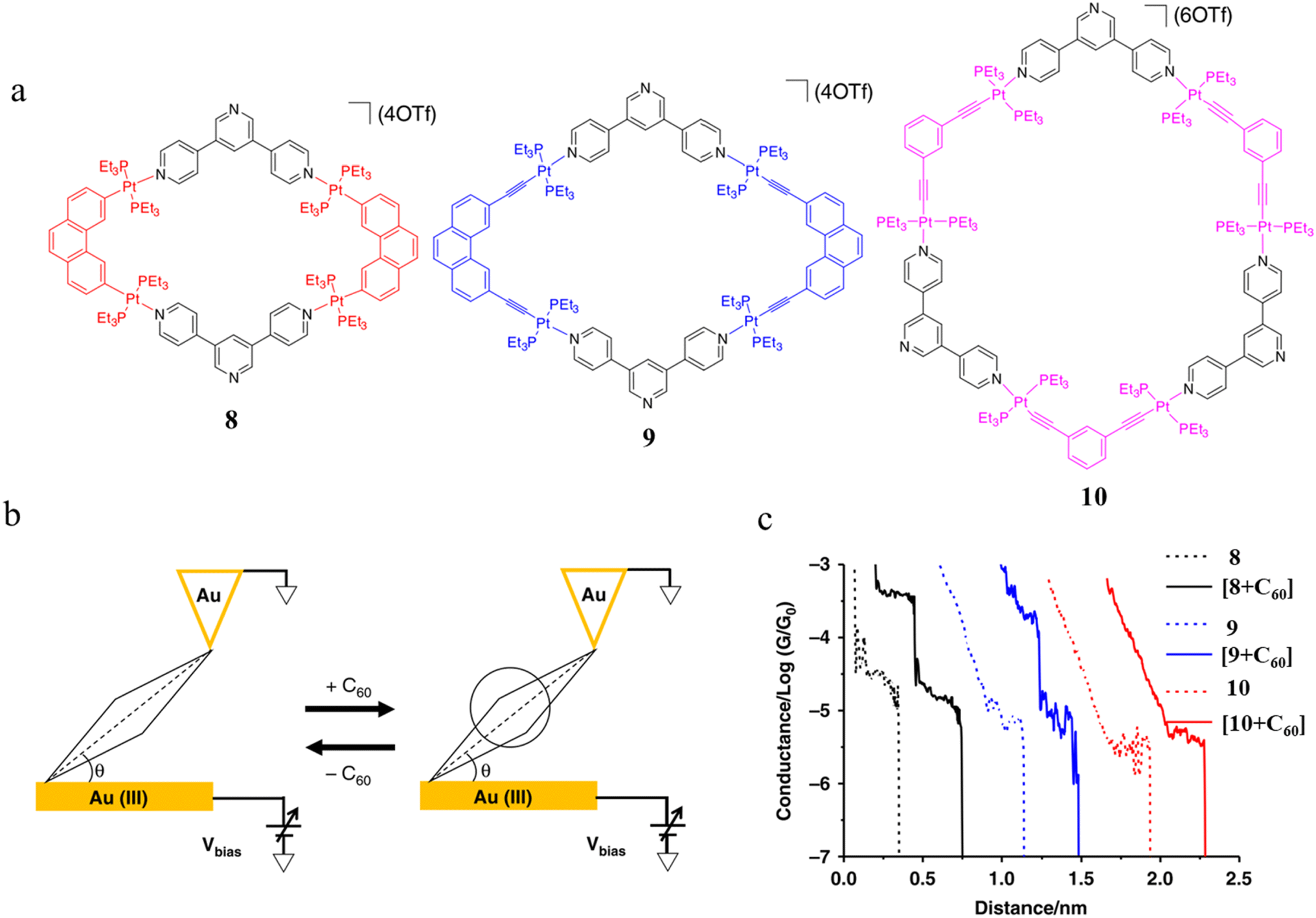 | ||
| Fig. 35 (a) Molecular structure of metallocycles 8, 9, and 10; (b) schematic of molecular junctions of metallocycles and those in the presence of C60; (c) conductance vs. distance traces of 8, 9 and 10, and [8 + C60], [9 + C60], 10 with C60. Figures adapted with permission from ref. 114. Copyright 2019, Springer Nature. | ||
Other examples of step-like transitions, from shorter, higher conductance plateaus to longer lower conductance plateaus have been discussed in Section 3.1.5 Supramolecular interaction.91–93,100,101,103
One such example of this unusual switching process can be found as a result of the in situ isomerisation of a spiro C–O bond in a spiropyran (Fig. 36a) covalently anchored to the electrodes during junction elongation.115 When the junction is extended, the spiropyran (SP) molecule within the junction slides into an upright position, at which point the application of further mechanical strain leads to the rupture of the C–O bond resulting in the mechanical formation of an isomeric, zwitterionic merocyanine (MC) ring-opened state. The more conjugated MC form, whilst longer than the parent SP, gives a higher molecular conductance and a step up in conductance immediately before the maximum junction length is exceeded and the junction breaks. This results in the appearance of a ‘spike’ at the end of the conductance plateau (Fig. 36b).
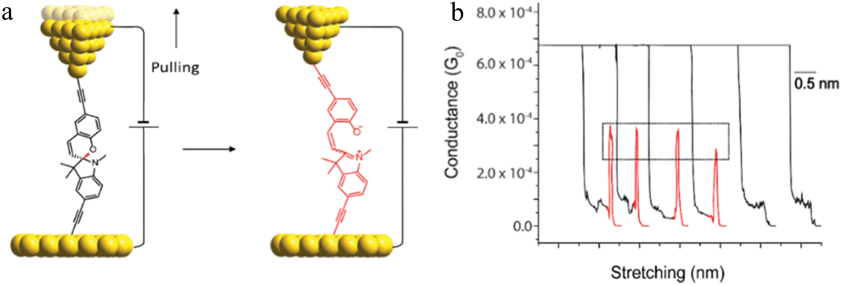 | ||
| Fig. 36 (a) Schematic of the stretching of a single spiropyran molecule during an STM-BJ experiment; (b) representative G–Δz curves of spiropyran with switching to a higher conductance level. Figures adapted with permission from ref. 115. Copyright 2019, American Chemical Society. | ||
Conductance spikes have also been attributed to changes in protonation state and contact binding during junction evolution.117 The compound 1,4-bis(1H-pyrazol-4-ylethynyl)benzene forms molecular junctions by chemisorbing on gold electrodes through the pyrazolyl group. Deprotonation a pyrazolyl moiety in the molecular junction leads to sudden jump in the conductance before the molecule detaches at the break-off distance and current dramatically decreases (Fig. 37a and b).117
 | ||
| Fig. 37 (a) Schematic of 1,4-bis(1H-pyrazol-4-ylethynyl)benzene junction; (b) a representative G–s trace obtained for 1,4-bis(1H-pyrazol-4-ylethynyl)benzene with high and low conductance point; (c) schematic of a BDT molecular junction; (d) a representative G–Δz trace of BDT with spike in conductance; (e) schematic energy diagram demonstrating how the energy of the HOMO changes relative to EF of the electrodes as electrode separation increases. Figures adapted with permission from ref. 117 and 118. Copyright 2018, American Chemical Society. Copyright 2011, Springer Nature Limited. | ||
The spikes observed in single-molecule conductance measurements of 1,4-benzenedithiol (BDT) with gold electrodes (Fig. 37c and d) has been attributed to force-induced resonant enhancement as the HOMO-related molecular states move that are located below the Fermi level of the gold electrodes in the relaxed junction configuration rise towards the Fermi level in the stretched junction due to decreased coupling between the molecule and electrodes (Fig. 37e).118 Repeated stretching and compressing reproduce this conductance increase and decrease without any hysteresis, suggesting a continuous stretching and relaxation in the bonds at the molecule–electrode contact, rather than a sudden rearrangement of contact geometry.
The EC-STM-BJ technique has been used to study the formation and evolution of single molecule and supramolecular dimer-based molecular junctions derived from 3,3′,5,5′-tetramethylbenzidine (TMB) and its redox products by controlling the potentials of the tip and the substrate relative to the reference electrode, leading to discovery of a further mechanism for jumps in molecular conductance.119 The cyclic voltammogram TMB is characterised by two well-behaved redox processes between 0–0.70 V (vs. Agwire) (Fig. 38a). The first one-electron oxidation corresponds to the conversion of the neutral molecule into a mixed-valence radical species, whilst the second process yields a diimine (Fig. 38b). Given the Nernstian equilibrium concentrations of the different redox forms within the junction under an applied electrochemical gate and the high concentration of TMB in the bulk solution, individual conductance traces exhibit distinct features at different electrochemical gate potentials (Fig. 38c). The high conductance, and relatively short plateaus observed from experiments conducted with electrochemical gate voltage of 0 V are attributed to single-molecule junctions formed from the neutral TMB molecule; the step to a lower conductance plateau of longer overall length is then attributed to formation of a supramolecular π–π stacked bimolecular junction formed as one molecule–electrode contact is ruptured. Similar long plateaus corresponding to bimolecular junctions are observed at gate potentials of 0.35 V but now attributed to the supramolecular structure formed by a radical and neutral form of TMB. This supramolecular radical structure has a conductance some order of magnitude higher than the simple π–π stacked neutral dimer and higher than the simple radical junction. Formation of a charge-transfer complex occurs when the diimine interacts with the original TMB substrate and the relatively low conductance features at 0.55 V are attributed to the supramolecular charge transfer complex.
 | ||
| Fig. 38 (a) CV of the TMB molecule and the redox products corresponding to the different potential regions; (b) mechanism of the electrochemical redox reaction for the TMB molecule; (c) individual conductance traces at different electrochemical gate potentials (0, 0.35 and 0.55 V); (d) 2D conductance histograms for TMB-based junctions at 0.35 V electrochemical gate potentials (insets: the corresponding relative stretching distance distributions of single-molecule junctions). Figures adapted with permission from ref. 119. Copyright 2023, American Chemical Society. | ||
Conductance jumps have also been observed in traces formed from indacenodithiophene with two 1,3-diethyl-2-thiobarbituric end groups (IDT-T) (Fig. 39a and b), and have been attributed to switching between Constructive Quantum Interference (CQI) and Destructive Quantum Interference (DQI) conductance pathways.69 AFM-BJ measurements indicated that these conductance jumps stemmed from alterations between the electrode contact at different anchoring sites along the molecular backbone (Fig. 39c). Aside from the thiono groups of the two 1,3-diethyl-2-thiobarbituric moieties, both the sulfur atom of the thiophene moiety and the nitrogen atom of the heterocycle possess the capacity to serve as anchoring sites onto the gold electrodes. Furthermore, precise mechanical tuning between conductance features was achieved by varying the dimension of the electrode gap and hence the most probable anchoring sites.
 | ||
| Fig. 39 (a) Chemical structure of IDT-T; (b) three types of typical individual conductance–displacement traces; (c) schematic of mechanical tuning of molecular conductance of IDT-T based on STM-BJ technique. Figures adapted with permission from ref. 69. Copyright 2023, Wiley-VCH GmbH. | ||
4. Junction formation probability
In addition to information concerning the various physical and chemical changes that take place after formation of a molecular junction contained within I–Δz (or G–Δz) curves, the frequency or probability of junction formation can also provide insight concerning the nature of molecule–electrode binding. In simplest terms, one might consider that more frequent junction formation events correlate with a higher molecule–electrode binding energy, and hence indicate stronger interactions between a molecule and the electrodes. Consideration of such ideas has prompted the report of the number of successfully formed molecular junctions as a percentage of the total number of traces recorded as the Junction Formation Probability (JFP). The JFP parameter has emerged as a powerful tool to investigate thermodynamic and kinetic aspects of junction formation. This section will discuss the factors that affect JFP, including the chemical nature of the anchor group and electrode material (and hence molecule–electrode binding energy),47 solvent,44,45 molecular length,133,140,141 molecular configuration,109,142,143 concentration,144,145 type of electrode metal,140,146 and external stimuli including applied bias,147,148 temperature,149–152 and light.153To illustrate the concept, consider the single molecule junctions formed from tolane (diphenylacetylene)-type molecules with different anchoring groups (SH, pyridyl (PY), NH2, and CN) (Fig. 40) and gold electrodes,47 for which the binding energies follow the sequence Au–S ≫ Au–PY > Au– CN > Au–NH2. The junction formation probabilities follow the sequence PY > S > CN > NH2, which is near identical to the binding energy sequence, except that PY and S are reversed. This suggests that the binding energy plays a major role in determining the junction formation probability. Other factors affecting the junction formation include the ability of a molecule to migrate into or within the junction, which in the case of sulfur-based contacts may be reduced if the higher binding energy decreases the mobility of the anchor in the vicinity of the Au tip.47 In the case of the pyridyl anchors, a significant π-face to gold component of the binding energy may also result in higher probability of formation as the analyte pre-assembles on the thinning gold filament.
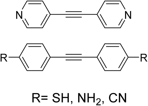 | ||
| Fig. 40 The tolane compounds used for investigation of JFP.47 | ||
In addition to anchor group chemistry, the solvent medium also affects the JFP,44,45 a process clearly demonstrated by STM-BJ measurements of 1,4-benzenediamine (BDA) as a solution in different solvents, augmented by calculations of the solvent–electrode binding interactions.45 It was found that JFP for DBA in chlorobenzene was 50%, in bromobenzene 45%, and in iodobenzene 0–30%. The JFP was considered as a consequence of competition between solvent and analyte for binding sites at undercoordinated Au atoms around the junction and explored through calculations of the energy barrier to replacement of a surface-bound BDA with a solvent molecule. Using a simple two-state Boltzmann model, it was found that the probability of displacing BDA varied from as low as 0.01 for chlorobenzene to 0.27 for bromobenzene to 0.99 for iodobenzene. Indeed, the weak binding energies associated with chlorobenzene which result in a low replacement probability point to the general inability of chlorinated solvents to replace BDA around the junction. For BDA dissolved in bromobenzene, the probability of displacement by the solvent is significant, leading to a significant competition between solvent and analyte for binding sites, and frequent binding dissociation events of the BDA within the junction. In contrast, the high BDA replacement probability of iodobenzene to the gold electrodes suggests that the probability of BDA junctions forming in this solvent will be low.45
Given the critical role of molecule–electrode binding on JFP, the nature of the electrode also plays a role in this parameter. For a series of amine-terminated oligophenyls and alkanes it was found that JFP was significantly higher for Ag electrodes than Au electrodes.140,141,154 For both Ag and Au electrodes, the probability of junction formation increases as the molecular backbone length increases (Fig. 41a and b). This was attributed to the smaller ‘snap back’ distance after rupture for Ag electrodes (0.5 nm) than Au electrodes (0.8 nm) (Fig. 41c),140 the assembly of the compounds along the thinning metal filament, and the greater capacity of the longer molecules to span wider range of break points along the filament.
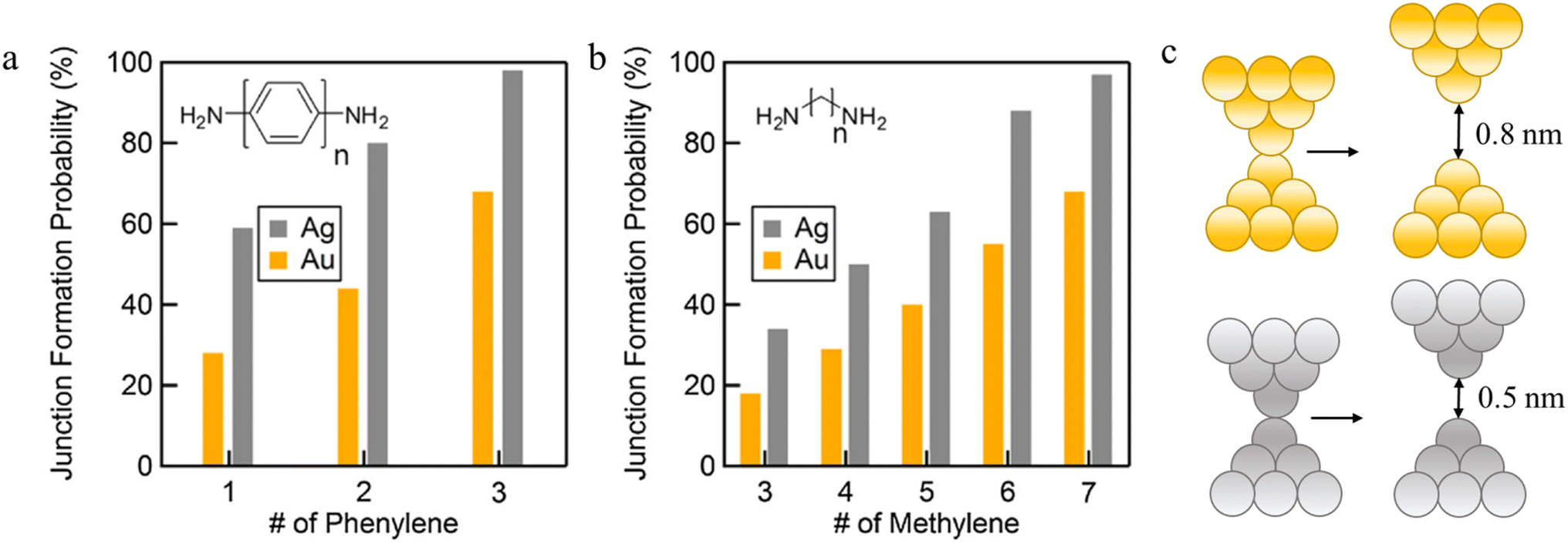 | ||
| Fig. 41 (a) Plots showing the JFP of the amine-terminated oligophenyl series; (b) plots showing the JFP of the amine-terminated alkane series; (c) Au (yellow) and Ag (grey) electrodes after contact ruptures with opening up a gap. Figures adapted with permission from ref. 140. Copyright 2015, Elsevier B.V. | ||
The opposite trend between length and JFP was found with trimethylsilylethynyl (TMS-ethynyl)-terminated oligo-(phenylene ethynylene) (OPE) molecules contacted to gold electrodes through covalent C–Au bonds formed as a result of in situ desilylation reactions (Fig. 42).133 This likely indicates the specific geometry of the molecule normal to the surface necessary to give rise to the Au|C![[triple bond, length as m-dash]](https://www.rsc.org/images/entities/char_e002.gif) C contact, with shorter molecules more readily inserted into the snap-backed gap that opens on cleavage of the metal filament.
C contact, with shorter molecules more readily inserted into the snap-backed gap that opens on cleavage of the metal filament.
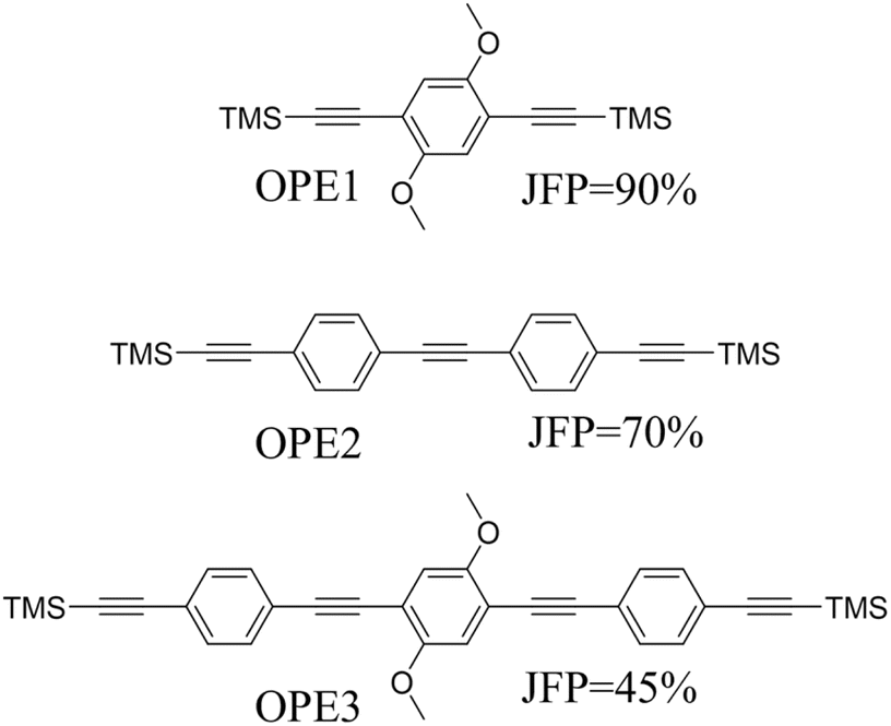 | ||
| Fig. 42 Structures of OPE1–OPE3 and the associated JFP determined from molecular junctions formed as a result of desilyation; TMS = trimethylsilyl, SiMe3.133 | ||
More broadly, in addition to the individual anchor atom–electron binding energies, geometric factors arising from interplay of the configuration of the molecular backbone and relative position of binding groups affect the ability of a molecule to bind to the electrode surface.109,142 Junction formation probability for six dithiomethyl phenanthrene (PHE-2SMe) with different position of binding groups (in positions 1,6-, 2,6-, 3,6-, 1,7-, 2,7-, 1,8-) has been estimated (Table 3).109 The molecules 1,8-PHE-2SMe and 3,6-PHE-2SMe have the lowest JFP likely due to steric constraints. The higher JFP associated with 1,7-PHE-2SMe and 2,6-PHE-2SMe can be attributed to the shift of the anchor group from the meta- to less constrained para-positions. This supposition is supported by the observation that among this series of compounds, 2,7-PHE-2SMe demonstrated the highest rate of junction formation (approximately 85%). Such ideas of geometric restrictions around the binding sites is also evident in the JFPs of a series of pyridyl-terminated oligo(phenylene ethynylene) molecules that differ in the relative para (p), meta (m) or ortho (o) locations of the nitrogen in the anchor units (Table 4).142 The JFP for molecules p–p–p, p–m–p, m–p–m and m–m–m reached 100%, reflecting the relatively sterically unrestricted anchor groups. However, for the molecule with o–p–o connectivity, in which the N-atoms of the terminal ortho pyridyl anchors are partially obstructed by the molecular backbone, the JFP decreased sharply to 21% in MCBJ measurements and 27% in STM-BJ experiments. The molecular conductance of the o–m–o falls below the limits of the noise floor, and as such no JFP information could be obtained.
| Structure | JFP, % (MCBJ) | JFP, % STM-BJ |
|---|---|---|
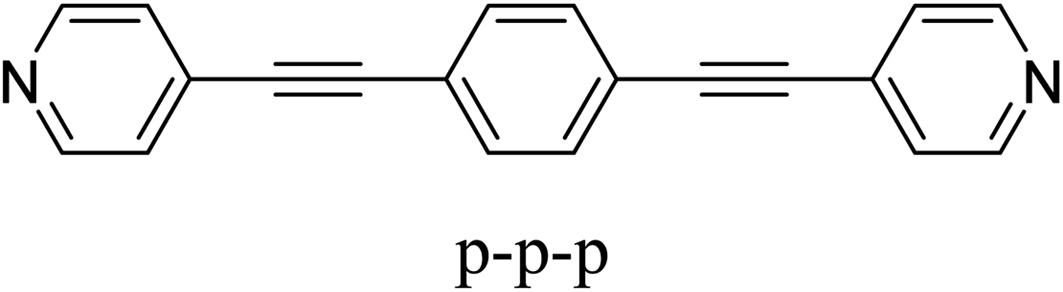
|
100 | 100 |
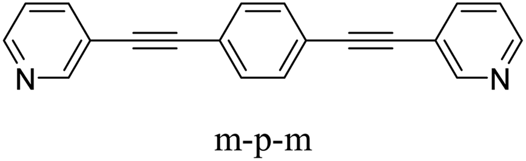
|
100 | 100 |
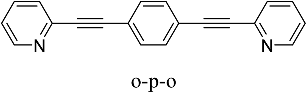
|
21 | 27 |
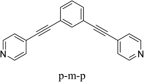
|
100 | 100 |
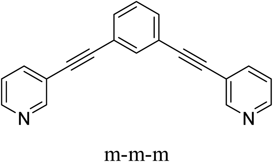
|
100 | No |
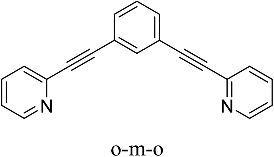
|
No | No |
A study of JFP as a function of analyte concentrate has been carried out with 1,4-bis((4-(methylthio)phenyl)ethynyl)benzene (OPE3-SMe), 1,4-bis(pyrid-4-yl)benzene (OAE2-PY) and 4,4-diamino-p-terphenyl (DATP-NH2), revealing an increase in JFP with increasing concentration (Fig. 43).144 Since the JFP of a molecular junction is proportional to the number of molecules adsorbed on the surface of the metal filament and ultimately the electrode surfaces, but not the free molecules in solution because only the molecules that are adsorbed on the electrode surface contribute to the formation of the molecular junction, this behaviour offers an opportunity to correlate the formation probability of molecular junction with the molecular adsorption free energy on the surface.144
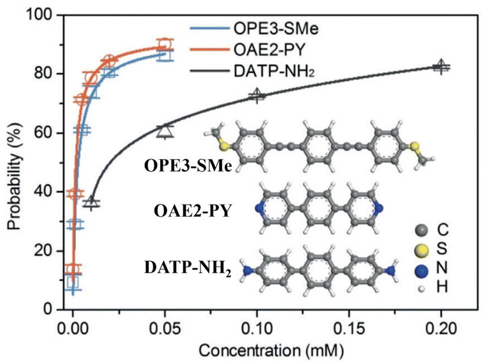 | ||
| Fig. 43 JFP as a function of molecular concentration for OPE3-SMe, OAE2-Py, and DATP-NH2. Figure adapted with permission from ref. 144. Copyright 2019, Wiley-VCH Verlag GmbH & Co. KGaA. | ||
The JFP of molecules 1,4-bis((4-(methylthio)phenyl)ethynyl)benzene (M1), (1E,1′E)-1,1′-(1,4-phenylene)bis(N-(4-(methylthio)phenyl)methanimine) (M2), 1,4-bis(((4-thioacetyl)phenyl)ethynyl)benzene (M3), 4,4-diamino-p-terphenyl (M4), and 1,4-bis(pyrid-4-yl)benzene (M5) with different anchors groups under external electric fields has been investigated (Fig. 44a).147 Results demonstrated that the JFP for molecules M1 and M2 with methylthioether (SMe) anchor groups increased as the applied bias increased from 20 to 250 mV. In contrast, molecule M3 with thiolate (introduced as the thioacetate, –SAc), M4 with amine (–NH2), and M5 with pyridyl (–PY) groups showed decreased JFP with increasing bias (Fig. 44b). The molecules M1 and M2 anchored to the electrodes through the terminal group of –SMe groups gave coupling strength closely associated with the molecular dipole moment. It was found that the configuration of –SMe anchored M1 and M2 evolved significantly as the external electric field increased with the relative conformations of the –SMe methyl groups driving changes in the molecular dipole moment to align with the increasing electric field across the junction. For M3, M4 and M5, it was found that the adsorption free energies of model junctions without external electric field are −23.58, −27.69, and −35.29 kJ mol−1, respectively. On the other hand, applying the electric field reduced adsorption free energies of M3–M5 to −10.88, −16.55, and −19.10 kJ mol−1, respectively, leading to the reduction of junction formation probability (Fig. 44b).155
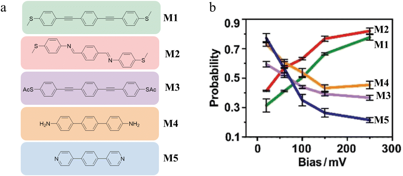 | ||
| Fig. 44 (a) Structures of M1–M5 highlighted in the colour corresponding to the JFP trend lines in (b); (b) plots of the junction formation probability of M1 (green), M2 (red), M3 (purple), M4 (orange), and M5 (blue) versus applied biases. Figures adapted with permission from ref. 155. Copyright 2020, Wiley-VCH Verlag GmbH & Co. KGaA. | ||
Zhan et al. demonstrated that JFP within an MCBJ arrangement can be controlled by changing the wavelength, polarization, and intensity of the incident light illuminating the gold nanotips in a solution of the analyte molecules (Fig. 45a).153 The interaction of the light with the thin gold filament (on the edge of the tip) causes the electrons on the metal surface to oscillate collectively creating an electromagnetic field around the gold filament (surface plasmon (SP) effect). The surface plasmons generate create an enhanced local electromagnetic field that helps to trap a molecule in the nanogap between gold electrodes. It was demonstrated that the JFP of 1,4-bis((4-(methylthio)phenyl)ethynyl)benzene (OPE3-SMe) in the dark (without illumination) was close to 30% with minor improvement under 514 nm illumination (Fig. 45b and c). When exposed to irradiation from a 691 nm laser, the JFP increased to 65% in line with the increased SP effects in gold at this wavelength. Further, the polarization of the 691 nm light source also impacted the JFP of OPE3-SMe (Fig. 45d). Incident light with horizontal polarization to the electrodes significantly improved the JFP from 30% to 45%. In contrast, under illumination with vertically polarized light, the formation probability of the molecular junction was similar to that without illumination proving that the trapping effect was mainly from SP. The JFP was also estimated as a function of the laser intensity, demonstrating that JFP increased with increasing intensity of the illumination source (Fig. 45e).153
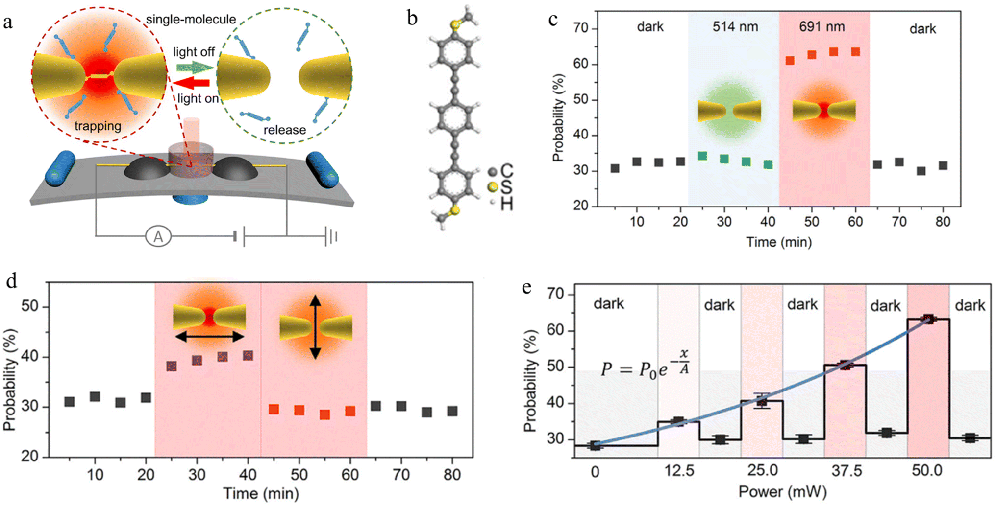 | ||
| Fig. 45 (a) Schematic of single-molecule plasmonic optical trapping; (b) structure of OPE3-SMe; (c) wavelength-controlled single-molecule trapping; (d) polarization-controlled single-molecule trapping; (e) JFP as a function of the laser intensity (691 nm−1). Figures adapted with permission from ref. 153. Copyright 2020, Elsevier. | ||
Finally, the probability of single-molecule junction formation increases with temperature as can be observed with higher counts in the 2D conductance histograms.149 Some studies suggested higher mobilities of Au atoms at higher temperatures make the formation of molecular junctions more likely with only minimal effect on molecular conductance.150–152
5. Machine learning for data analysis
Although 1D and 2D histograms are commonly used to analyse single-molecule measurements, these plots arise from a convolution of data including: traces with no molecular conductance signals; unstable traces due to physical or electronic instabilities of the instrument; traces with molecule-like features from contaminants in the solution or analyte; and all of the various individual junctions that can form from any given analyte. Together, these scenarios give rise to a myriad of different conductance plateaus in different conductance regions depending on binding configuration, conformation etc. all of which combine to give the features observed in the histograms.A compilation of all types of traces within a histogram therefore gives an average picture and a most probable conductance estimate, but the unique information from each trace is lost. To explore the body of data with more detail or precision, some filtering, selection, extraction, partitioning or clustering of traces is required by manual67,78,156–158 or automated143,159–164 means. Manual sorting of traces according to distinct features associated with the plateau shape is recognised as at risk of operator bias, as well as being extraordinarily time-consuming; consequently, automated feature extraction using machine-learning (ML) algorithms that minimise cognitive bias and are more time effective are being increasingly developed and adopted.
Generally, automated analysis of data consists of two main points: a method or approach that answers the question ‘what needs to be done with the data?’, for example, parameterisation and extraction of different features of the conductance trace or correlation of 1D and 2D histograms; and an appropriate algorithm that addresses the question ‘how it will be done?’, for example, by algorithms implemented in supervised or unsupervised ML methods.
Three broad approaches to the challenges of automating data analysis are illustrated in Fig. 40. In a clusters by parameters approach, the data are initially sorted on the basis of some parameterisation of the data by specific qualities;165–167 for example, conductance traces can be divided into linear segments that are parameterised on the basis of location, length, and angle of segment (Fig. 46, left block). Based on the parameters each segment is assigned to one of a number of different clusters, resulting in differentiation and categorisation of the various traces, and attributed to a distinct junction type.167 Another approach is a correlation of a matrix of data from 1D162 and 2D168 histograms compiled from individual traces. For example, each conductance trace can be plotted into individual 1D histograms (Fig. 46, middle block).162 Next, from the 1D histogram data, a matrix is produced. Subsequently principal component analysis (PCA) is used to identify axes with the biggest variation in the data identifying most important pattern and assign it to corresponding group.162
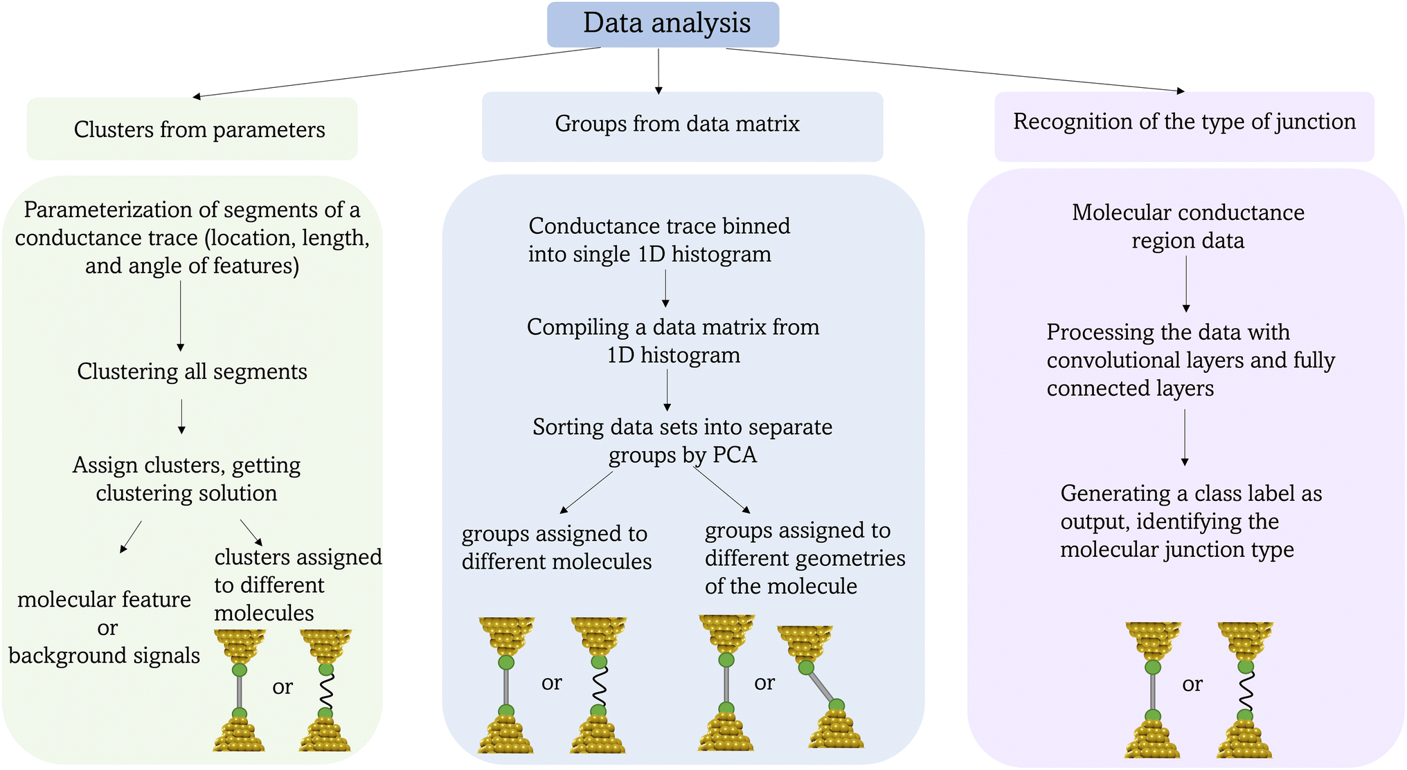 | ||
| Fig. 46 Schematic illustrating the more common approaches of machine learning in single-molecule conductance analysis. | ||
Alternatively, individual traces can be assigned to a different class of junction based on an image recognition technique.161,163,169 For example, each one of a series of traces from I(t) measurements has been converted into the corresponding images (Fig. 46, right block).163 These images were then passed through the feature extractor component of pre-trained image recognition networks. First, convolutional layers extract features from the image of the conductance trace. Then, fully connected layers find patterns and correlations in the extracted features allowing assignment of the image of the I–t trace to a specific class.163
The above general methods have been implemented within different machine learning algorithms that can be broadly categorised in terms of either supervised and unsupervised learning. Supervised learning is used when the nature of the desired machine-learning model output is known, whereas unsupervised learning is used, for example, to detect the underlying (and unknown) structures of a given data set.
5.1 Supervised machine learning
Supervised learning refers to the training of a computer algorithm to classify unknowns based on properties of known samples. Two primary types of supervised ML applied for analysis of molecular conductance data are regression25,170–173 (Fig. 47a) and classification169,174–176 (Fig. 47b). The main difference between those two algorithms is that regression predicts a continuous numerical value as the output variable, while classification aims to assign input instances to predefined categories or classes. The goal of regression is to find a mathematical function that best fits the data and can be used to make predictions of behaviour from a set of given inputs.170 The most used method is linear regression due its simplicity.25 The goal of classification is to build a model that can accurately predict the class or category based on patterns and relationships learned from the labelled dataset. The model learns from the examples in the training data. Machine learning classification is widely employed in image recognising.174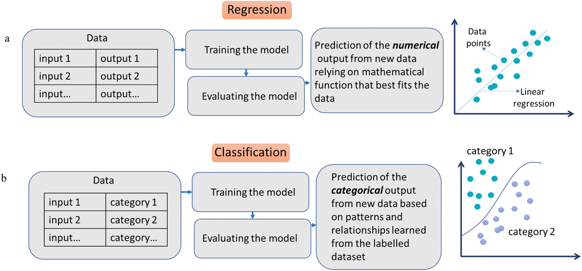 | ||
| Fig. 47 Schematic of (a) linear regression and (b) classification in machine learning. | ||
5.2 Unsupervised machine learning
In unsupervised learning, algorithms are not provided with labels, instead, they directly estimate the probability density of the data based on the measured information. The evaluation of unsupervised learning results often relies on physical interpretations, and validation methods tend to be heuristic in nature. In the context of single-molecule measurements, the main unsupervised learning technique is clustering (Fig. 48).159,160,177,178 Clustering is a technique used to group similar data points together based on their characteristics or features. The goal of clustering is to identify patterns or structures in a dataset without any prior knowledge or labels.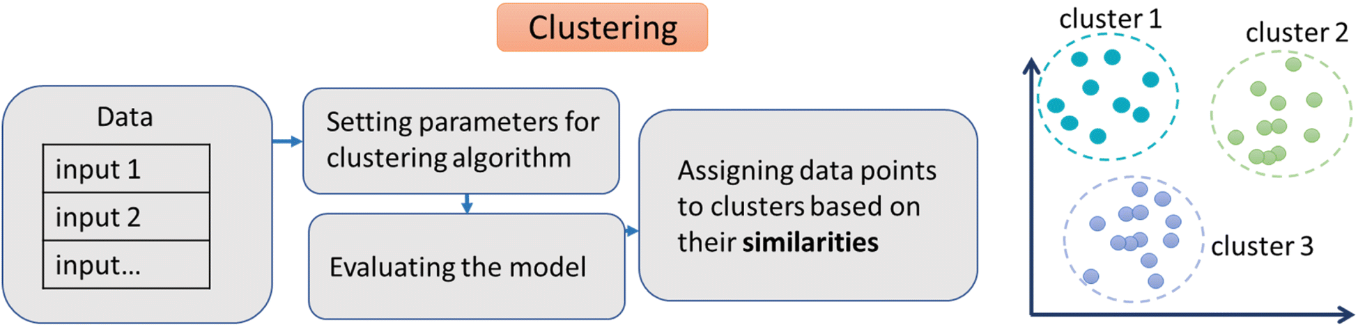 | ||
| Fig. 48 Schematic of clustering in machine learning. | ||
Recently, XMe Code (Xiamen Molecular Electronics Code), an intelligent all-in-one data open-source analysis tool for the comprehensive analysis of single-molecule break junction data has been published. The code is based on unsupervised clustering algorithm and have been tested on more than 20 set-ups among more than 10 research laboratories is also carried out to demonstrate the reproducibility of the single-molecule conductance measurement using the XMe Code.179
6. Predictive ‘tools’
From the body of experiential data, models of single-molecule conductance have been developed. Although the description of a molecular junction is a complex, multi-parameter problem, these models are now sufficiently advanced to permit good accuracy in many a priori predictions of electrical properties of single molecules. Of equal merit, the accuracy of these models allows a range of molecular junction scenarios to be explored and compared against experimental results to help rationalise observations.When developing a predictive model of molecular conductance, the energy barrier (Emol) between the electrode Fermi level and the energy level(s) within the molecule can be considered to provide an initial basis for a tunnelling model based description (Fig. 49). However, when a molecule is bonded to the electrodes in a molecular junction, the discrete molecular energy levels shift and broaden to an extent determined by the degree of electronic coupling, the extent to which is highly sensitive to the electrode material, the chemical composition of the anchor group and junction geometry. To a first approximation, electron transport through a single-molecule junction therefore depends on: the energy barrier, Emol, given by the energy difference between the frontier levels of the molecule (HOMO/LUMO) and the Fermi level EF in the electrodes; and the coupling strength Γ, between the molecular state and the electrodes.33 This section considers some of the predictive approaches most commonly found in the literature to date, and the basis for their application.
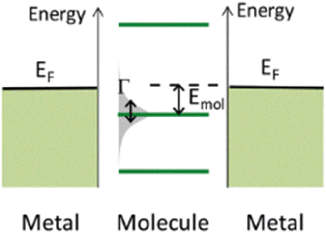 | ||
| Fig. 49 Energy level diagram for a single-molecule junction. The frontier level is the HOMO (with illustrated broadening), EF is Fermi level, and Emol is the energy barrier. Figure adapted with permission from ref. 33. Copyright 2014, American Chemical Society. | ||
6.1 Density functional theory
In general case of non-resonant transport, the current flowing through a molecular junction (Fig. 50a) is described by the expressions drawn from the Landauer or Landauer–Büttiker model (eqn (3)) | (3) |
 | ||
| Fig. 50 (a) Schematic of molecule junction consisting of right electrode, molecule, and left electrode. The molecule in molecular junction consists of anchor groups and a backbone; (b) schematic of transmission function T(EF). The Landauer models employ the concept of the transmission coefficient, T(E), which describes the probability of an electron wave of energy E propagating between probes connected to the channel. By evaluating T(EF), the transmission coefficient at the Fermi energy it is possible to extract the conductance (G) of the junction. | ||
While DFT-based methods are powerful tool for prediction Emol,182,183 the quantitative prediction of Emol requires a many-electron approach.184,185 The DFT + Σ method, developed by Quek and Neaton, relies on incorporating many-electron effects without the computational cost.111,186,187 DFT + Σ utilizes mean-field DFT to obtain the charge density for scattering states using a modified Hamiltonian with a self-energy correction operator Σ. In this appraoch, Σ is split into local and nonlocal contributions, accounting for changes in molecular levels due to charge transfer, chemical bonding, and renormalization effects from the metal surface.188 The DFT + Σ approach has shown significant improvement in predicting conductance values for different amine-Au and pyridine-Au single-molecule junctions compared to standard DFT methods.188 The DFT + Σ approach has successfully predicted conductance trends and thermopower as well as identified complex structure–conductance relationships by sampling various geometries. While DFT transport methods have provided qualitative estimation, the DFT + Σ approach relies on many-electron formalisms to accurately predict conductance and low bias I–V characteristics in the coherent tunneling regime.188,189 However, this approach is currently limited to intact single-molecule junctions, excluding widely studied thiol-Au junctions where the molecular S–H bond broken upon reaction with Au.118 Nevertheless, DFT based approaches are sufficiently well advanced, including the provision of user-friendly codes such as SMEAGOL182,190 and GOLLUM,110,180 that most studies of molecular junctions are accompanied on some level by such calculations.
Overall, DFT-based methods have proven to be a robust tool for exploration the electrical properties of molecular junctions. However, DFT methods cannot accurately predict the relative energies of the molecular orbital energies and the electrode Fermi levels, EF, which is critical to the prediction of molecular conductance, G. Thus, common practice in the field is to use the results of experimental measurements of molecular conductance to help determine the position of the Fermi level relative to transport resonances arising from, for example, the molecular HOMO and LUMO.
6.2 Quantum circuit rules
Although analytical methods and atomistic descriptions of junctions using DFT based methods have proven to be immensely powerful, there is still a strong desire to develop more empirical rules that account for molecular electronic properties in a simple fashion and permit ready estimation. Recently a qualitative method to predict molecular conductance has been proposed: this Quantum Circuit Rule (QCR) commences with a partition of the molecular junction into a series of weakly coupled scattering regions, each described by an independent numerical parameter.37 The rules most usefully apply to non-resonant tunnel junctions (i.e. the Fermi energy of the electrodes falls near the middle of the molecular HOMO–LUMO gap) formed from a molecule of general form X–B–Y (where X and Y are the anchor groups that bind the molecule to the electrodes and B is the molecular backbone, Fig. 51), with conductance dominated by coherent tunneling (i.e. molecules less than ca. 3 nm in length). | ||
| Fig. 51 A cartoon of a molecular X–B–Y junction with conceptual partitioning into anchor groups (X and Y) and the molecular backbone (B). | ||
Dyson's equation for the Green's function of a three serially connected subsystems X, B, and Y has been written as
 | (4) |
| GYX = gYV†YGBBV†XgX | (5) |
| TXBY = ℏν|[gYV†Y]ik|2|[GBB]|kl2ℏν|[V†XgX]lj|2 = AYBBAX | (6) |
The bridge parameter BB depends on X and Y through the self-energies VXgXV†X and V†YgYVY. If the Fermi energy does not coincide with the poles of gX and gY then Σ can be negligible and eqn (6) can be rewritten as
| TXBY2 = TXBXTYBY | (7) |
| GXBY2 = GXBXGYBY | (8) |
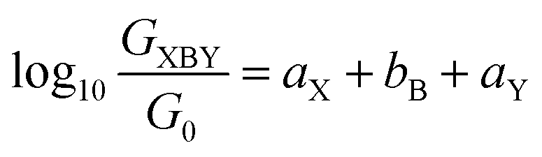 | (9) |
This QCR (eqn (9)) has been used to obtain parameters (aX,Y, bB) for some of the most common anchor groups and backbones (Tables 5 and 6) from the DFT-computed conductance of 180 molecules expanded by the experimentally determined conductance of a further 19 molecules.37
| Anchor |

|
|
|
|
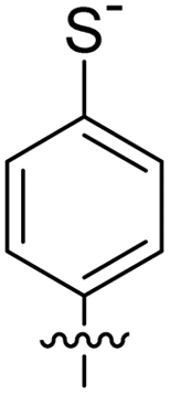
|
| a DFTX,Y | −1.12 | −0.89 | −1.20 | −0.87 | −0.68 |
| Backbone | b DFTB | Backbone | b DFTB |
|---|---|---|---|
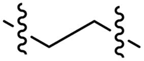
|
−2.04 |
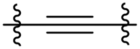
|
−0.12 |
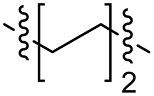
|
−4.57 |
|
−0.25 |
|
−5.19 |
|
−0.38 |
|
−0.09 |
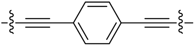
|
−0.73 |

|
−0.22 |
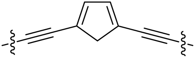
|
−0.46 |
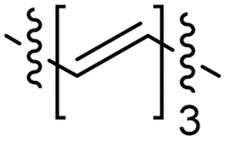
|
−0.35 |
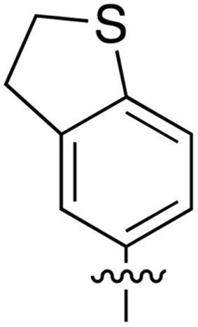
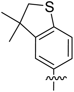
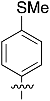
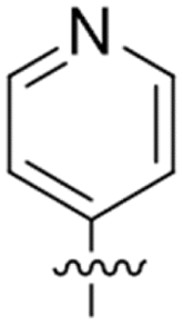
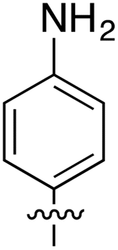
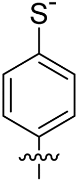
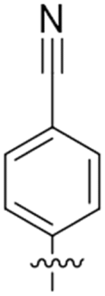
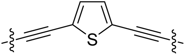
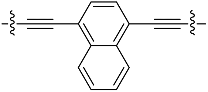
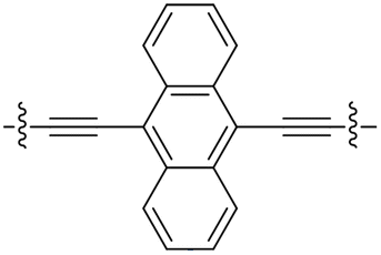
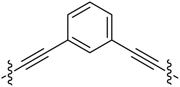
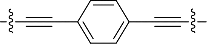
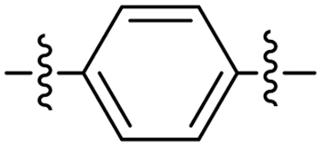
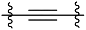
Anchor group parameters for the 3,3-dimethyl-2,3-dihydrobenzo[b]thiophene and thioanisole anchors have been identified from experimental conductance values determined from tolane compounds,35 whilst oligo(arylene-ethynylene)-molecular wires 6a–c, 7a–c, and 8a–c have been used to determine new backbone parameters (Fig. 52).36 Thus, from experimental conductance data and the relevant anchor group parameters, aX (Table 6), and the relationships contained in the QCR (eqn (9)) it was possible to calculate backbone parameters, bB, for the 2,5-diethynylthiophene (bthioph), 1,4-diethynylnaphthalene (bnaphth) and 9,10-diethynylanthracene (banth) fragments. In the same manner the backbone parameters, bB, for the various homologous members of the polyyne series (Fig. 53) (bCC, bCCCC, bCCCCCC and bCCCCCCCC) have been obtained (Table 6).38
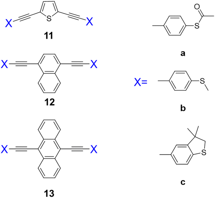 | ||
| Fig. 52 The structures of the OAE compounds used to provide estimates of backbone parameters, bB.36 | ||
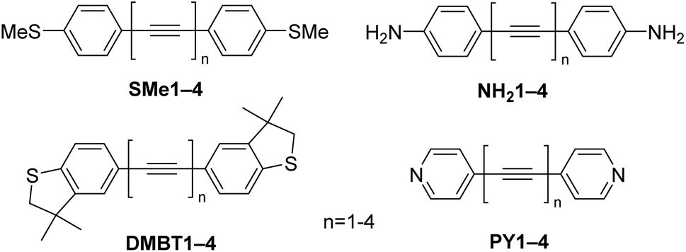 | ||
| Fig. 53 The structures of the polyyne derivatives used to provide estimates of the polyyndiyl backbone parameters, bB.38 | ||
Furthermore, the aX,Y parameters derived from several common anchor groups have been compared with contact conductance G2CN derived from polyynes featuring these anchors and for which structure–property relationships contained in the conductance data can be interpreted as a function of the number of repeat units in the molecular backbone, N, expressed as
| G = G2CNe−βNN | (10) |
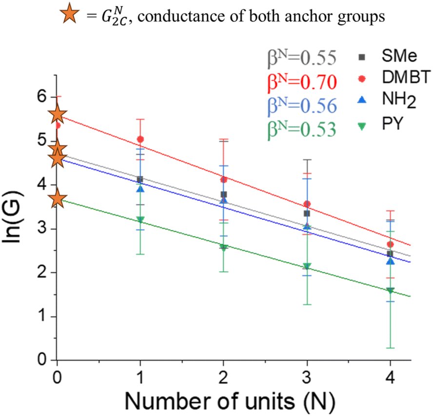 | ||
| Fig. 54 Plot of the most probable experimental conductance values ln(G) versus number of units –{CC–}, N, from STM-BJ measurements of the compounds shown in Fig. 53, conducted in mesitylene.38 | ||
| Compound | log(Gexp/G0) (solvent)a | log(G2CN/G0) | 2ax |
|---|---|---|---|
| a TCB = 1,2,4-trichlorobenzene; TMB = 1,3,5-trimethylbenzene (mesitylene). | |||
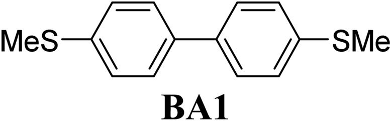
|
−2.80 (TCB)194 | −2.84 | −2.82 |
| −2.90 (TCB)169 | |||
| −2.89 (TCB)149 | |||
| −2.75 (TCB)195 | |||
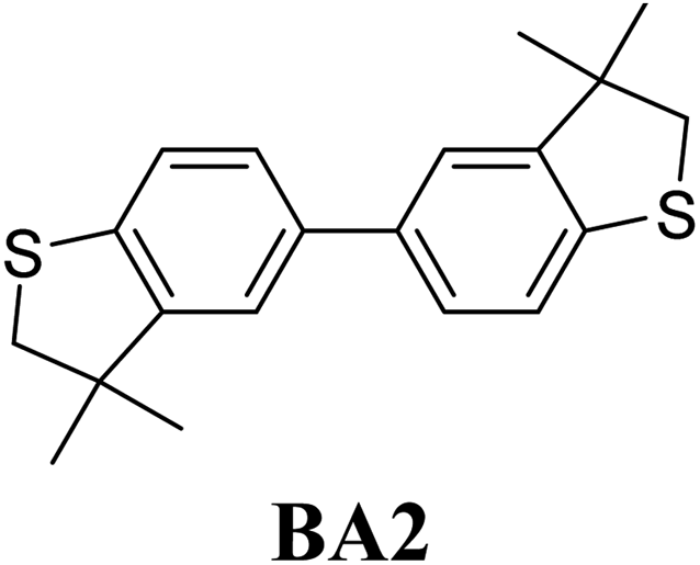
|
−2.56 (TMB)38 | −2.46 | −2.42 |
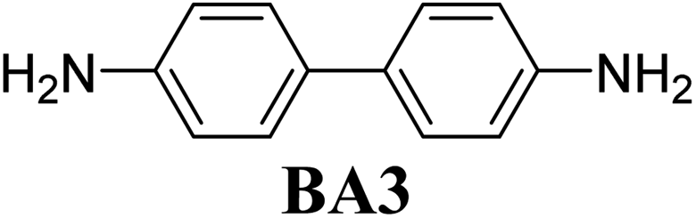
|
−2.95 (TCB)195 | −2.89 | −2.88 |
| −2.85 (TCB)10 | |||
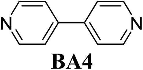
|
−3.30 (TCB)196 | −3.29 | −3.16 |
| −3.30 (unknown)197 | |||
| −3.35 (TCB)198 | |||
| −3.30 (TCB)111 | |||
Excellent agreement was found between anchor groups conductance value (G2CN) obtained from extrapolation of the data shown in Fig. 54, the previously determined anchor parameters, aX, and the experimentally determined values of molecular conductance of the biaryls BA1–BA4. This excellent agreement between experiment and the predictions of the QCR is due in part to the non-planar structure of biaryls, which limits conjugation between the two rings and allows approximation of the structure as two weakly coupled scattering sites.
The QCR has also been tested on a series of ‘modular’ molecular circuits, with various chemical ‘components’ assembled in series with different anchors at each terminus (Fig. 55). The single molecule conductance has been estimated from eqn (11) that allows molecular structure to be partitioned into a number of smaller scattering regions:
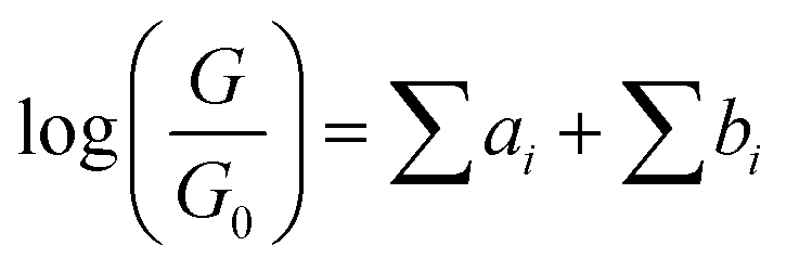 | (11) |
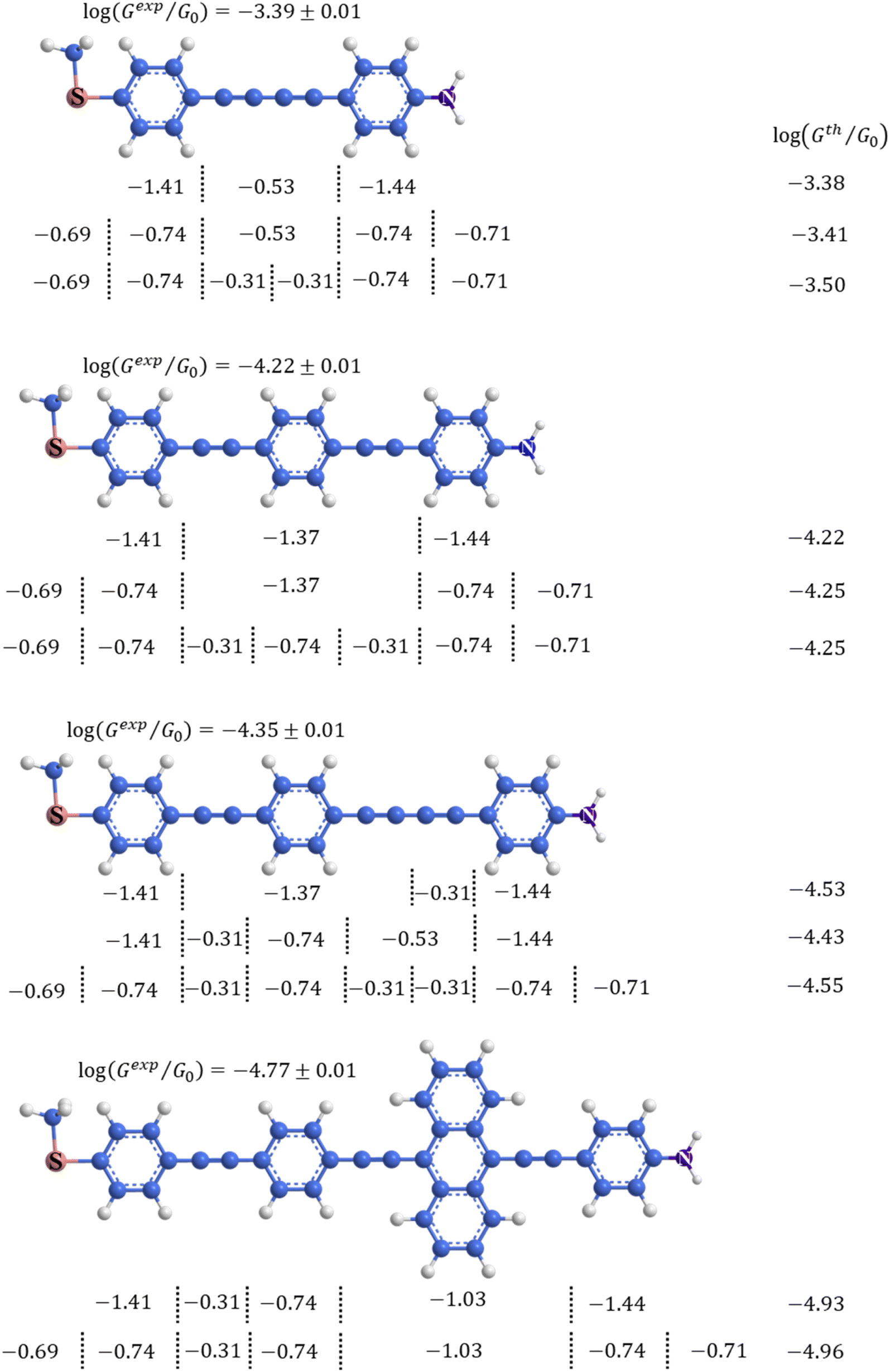 | ||
| Fig. 55 Schematics of compounds illustrating various partitioning strategies dividing the molecule into separate ‘components’ of the anchor groups and backbone fragments for which ai and bB parameters are known, assembled in series, the resulting calculated conductance values (log(GTh/G0)) from the QCR (eqn (11)) and experimentally determined values from STM-BJ measurements (log(GExp/G0)).38 | ||
The accuracy of these estimates (log(GTh/ G0)) have been tested against the single-molecule conductance of authentic samples (Fig. 55).
7. Conclusion
This overview has summarised some of the most common single-molecular junction fabrication techniques, interpretation of single molecular junction current distance traces, as well as some theoretical simulations. From current or conductance–distance traces, the plateau length, and the shape of the conductance plateau provide information concerning the different physical and chemical processes that take place in the junction during measurements. This information provides insight into the behaviour of the junction and understanding of single-molecule chemistry. To aid analyses, the diverse data from any single-molecule conductance measurement can be categorised and effectively sorted to the different classes by the machine learning algorithms. DFT-based methods have proven to be a robust tool for further exploration of the electrical properties of molecular junctions and with computational models proving essential to the determination of molecular level detail and rationalisation of observations. However, DFT methods cannot accurately predict the relative energies of the molecular orbital energies and the electrode Fermi levels, EF, which is critical to the prediction of molecular conductance. To this end the Quantum Circuit Rules offers simple fashion and permit ready estimation of the single-molecular conductance and could be a useful empirical tool for explaining unexpected conductance features in complex conductance data.Author contributions
E. G. drafted the text and participated in the editing of the final manuscript. P. J. L. conceived the project, supervised the work and edited the drafts.Conflicts of interest
There are no conflicts to declare.Acknowledgements
The authors gratefully acknowledge support for our work in this area from the Australian Research Council Discovery Program (DP220100790).References
- S. Marques-Gonzalez and P. J. Low, Aust. J. Chem., 2016, 69, 244–253 CrossRef CAS.
- D. Xiang, X. Wang, C. Jia, T. Lee and X. Guo, Chem. Rev., 2016, 116, 4318–4440 CrossRef CAS PubMed.
- A. Jain and S. J. George, Mater. Today, 2015, 18, 206–214 CrossRef CAS.
- O. T. Gül, K. M. Pugliese, Y. Choi, P. C. Sims, D. Pan, A. J. Rajapakse, G. A. Weiss and P. G. Collins, Biosensors, 2016, 6, 29 CrossRef PubMed.
- H. Chen and J. Fraser Stoddart, Nat. Rev. Mater., 2021, 6, 804–828 CrossRef CAS.
- T. C. Siu, J. Y. Wong, M. O. Hight and T. A. Su, Phys. Chem. Chem. Phys., 2021, 23, 9643–9659 RSC.
- T. A. Su, M. Neupane, M. L. Steigerwald, L. Venkataraman and C. Nuckolls, Nat. Rev. Mater., 2016, 1, 16002 CrossRef CAS.
- P. Gehring, J. M. Thijssen and H. S. J. van der Zant, Nat. Rev. Phys., 2019, 1, 381–396 CrossRef.
- B. Xu and N. J. Tao, Science, 2003, 301, 1221–1223 CrossRef CAS PubMed.
- L. Venkataraman, J. E. Klare, C. Nuckolls, M. S. Hybertsen and M. L. Steigerwald, Nature, 2006, 442, 904–907 CrossRef CAS PubMed.
- M. S. Hybertsen and L. Venkataraman, Acc. Chem. Res., 2016, 49, 452–460 CrossRef CAS PubMed.
- C. J. Muller, J. M. van Ruitenbeek and L. J. de Jongh, Phys. C, 1992, 191, 485–504 CrossRef.
- R. H. M. Smit, Y. Noat, C. Untiedt, N. D. Lang, M. C. van Hemert and J. M. van Ruitenbeek, Nature, 2002, 419, 906–909 CrossRef CAS PubMed.
- M. A. Reed, C. Zhou, C. J. Muller, T. P. Burgin and J. M. Tour, Science, 1997, 278, 252–254 CrossRef CAS.
- D. J. Wold and C. D. Frisbie, J. Am. Chem. Soc., 2000, 122, 2970–2971 CrossRef CAS.
- Z. Li, L. Mejía, J. Marrs, H. Jeong, J. Hihath and I. Franco, J. Phys. Chem. C, 2021, 125, 3406–3414 CrossRef CAS.
- W. Haiss, C. Wang, I. Grace, A. S. Batsanov, D. J. Schiffrin, S. J. Higgins, M. R. Bryce, C. J. Lambert and R. J. Nichols, Nat. Mater., 2006, 5, 995–1002 CrossRef CAS PubMed.
- T. Markussen, J. Schiötz and K. S. Thygesen, J. Chem. Phys., 2010, 132, 224104 CrossRef PubMed.
- C. Li, I. Pobelov, T. Wandlowski, A. Bagrets, A. Arnold and F. Evers, J. Am. Chem. Soc., 2008, 130, 318–326 CrossRef CAS PubMed.
- R. Ramachandran, H. B. Li, W. Y. Lo, A. Neshchadin, L. Yu and J. Hihath, Nano Lett., 2018, 18, 6638–6644 CrossRef CAS PubMed.
- C. Tang, R. T. Ayinla and K. Wang, J. Mater. Chem. C, 2022, 10, 13717–13733 RSC.
- H. Chen, C. Jia, X. Zhu, C. Yang, X. Guo and J. F. Stoddart, Nat. Rev. Mater., 2023, 8, 165–185 CrossRef.
- A. Vladyka, M. L. Perrin, J. Overbeck, R. R. Ferradás, V. García-Suárez, M. Gantenbein, J. Brunner, M. Mayor, J. Ferrer and M. Calame, Nat. Commun., 2019, 10, 262 CrossRef PubMed.
- L. Mejía, P. Cossio and I. Franco, Nat. Commun., 2023, 14, 7646 CrossRef PubMed.
- W. Bro-Jørgensen, J. M. Hamill, R. Bro and G. C. Solomon, Chem. Soc. Rev., 2022, 51, 6875–6892 RSC.
- H. Song, Y. Kim, H. Jeong, M. A. Reed and T. Lee, J. Phys. Chem. C, 2010, 114, 20431–20435 CrossRef CAS.
- H. Oberhofer, K. Reuter and J. Blumberger, Chem. Rev., 2017, 117, 10319–10357 CrossRef CAS PubMed.
- C. J. Lambert, Quantum Transport in Nanostructures and Molecules: An Introduction to Molecular Electronics, IOP Publishing, Bristol, UK, 2021 Search PubMed.
- C. J. Lambert, Chem. Soc. Rev., 2015, 44, 875–888 RSC.
- K. R. Parenti, R. Chesler, G. He, P. Bhattacharyya, B. Xiao, H. Huang, D. Malinowski, J. Zhang, X. Yin, A. Shukla, S. Mazumdar, M. Y. Sfeir and L. M. Campos, Nat. Chem., 2023, 15, 339–346 CrossRef CAS PubMed.
- D. A. Egger, Z. F. Liu, J. B. Neaton and L. Kronik, Nano Lett., 2015, 15, 2448–2455 CrossRef CAS PubMed.
- C. Jin, M. Strange, T. Markussen, G. C. Solomon and K. S. Thygesen, J. Chem. Phys., 2013, 139, 184307 CrossRef PubMed.
- S. Y. Quek and K. H. Khoo, Acc. Chem. Res., 2014, 47, 3250–3257 CrossRef CAS PubMed.
- V. Coropceanu, J. Cornil, D. A. d. S. Filho, Y. Olivier, R. Silbey and J.-L. Bredas, Chem. Rev., 2007, 107, 926–952 CrossRef CAS PubMed.
- E. Gorenskaia, M. Naher, L. Daukiya, S. Moggach, D. C. Milan, A. Vezzoli, C. Lambert, R. Nichols, T. Becker and P. J. Low, Aust. J. Chem., 2021, 74, 806–818 CrossRef CAS.
- M. Naher, E. Gorenskaia, S. A. Moggach, T. Becker, R. J. Nichols, C. J. Lambert and P. J. Low, Aust. J. Chem., 2022, 75, 506–522 CrossRef CAS.
- D. Z. Manrique, Q. Al-Galiby, W. Hong and C. J. Lambert, Nano Lett., 2016, 16, 1308–1316 CrossRef CAS PubMed.
- E. Gorenskaia, J. Potter, M. Korb, C. Lambert and P. Low, Nanoscale, 2023, 15, 10573–10583 RSC.
- Y. Zhao, W. Liu, J. Zhao, Y. Wang, J. Zheng, J. Liu, W. Hong and Z. Q. Tian, Int. J. Extreme Manuf., 2022, 4, 022003 CrossRef CAS.
- A. Vilan, D. Aswal and D. Cahen, Chem. Rev., 2017, 117, 4248–4286 CrossRef CAS PubMed.
- E. Leary, A. La Rosa, M. T. González, G. Rubio-Bollinger, N. Agraït and N. Martín, Chem. Soc. Rev., 2015, 44, 920–942 RSC.
- J. Liu, X. Zhao, J. Zheng, X. Huang, Y. Tang and F. Wang, Chem, 2019, 5, 390–401 CAS.
- C. Tang, T. Stuyver, T. Lu, J. Liu, Y. Ye, T. Gao, L. Lin, J. Zheng, W. Liu, J. Shi, S. Shaik, H. Xia and W. Hong, Nat. Commun., 2023, 14, 3657 CrossRef CAS PubMed.
- Š. Nováková Lachmanová, V. Kolivoška, J. Šebera, J. Gasior, G. Mészáros, G. Dupeyre, P. P. Lainé and M. Hromadová, Angew. Chem., Int. Ed., 2021, 60, 4732–4739 CrossRef PubMed.
- V. Fatemi, M. Kamenetska, J. B. Neaton and L. Venkataraman, Nano Lett., 2011, 11, 1988–1992 CrossRef CAS PubMed.
- Y. Zhu, Z. Tan and W. Hong, ACS Omega, 2021, 6, 30873–30888 CrossRef CAS PubMed.
- W. Hong, D. Z. Manrique, P. Moreno-García, M. Gulcur, A. Mishchenko, C. J. Lambert, M. R. Bryce and T. Wandlowski, J. Am. Chem. Soc., 2012, 134, 2292–2304 CrossRef CAS PubMed.
- T. Fu, K. Frommer, C. Nuckolls and L. Venkataraman, J. Phys. Chem. Lett., 2021, 12, 10802–10807 CrossRef CAS PubMed.
- C. A. Martin, D. Ding, J. K. Sørensen, T. Bjørnholm, J. M. Van Ruitenbeek and H. S. J. Van Der Zant, J. Am. Chem. Soc., 2008, 130, 13198–13199 CrossRef CAS PubMed.
- S. V. Aradhya and L. Venkataraman, Nat. Nanotechnol., 2013, 8, 399–410 CrossRef CAS PubMed.
- C. Huang, A. V. Rudnev, W. Hong and T. Wandlowski, Chem. Soc. Rev., 2015, 44, 889–901 RSC.
- W. Haiss, R. J. Nichols, H. Van Zalinge, S. J. Higgins, D. Bethell and D. J. Schiffrin, Phys. Chem. Chem. Phys., 2004, 6, 43330–44337 RSC.
- E. M. Dief and N. Darwish, Chem. Sci., 2023, 14, 3428–3440 RSC.
- W. Haiss, H. Van Zalinge, S. J. Higgins, D. Bethell, H. Höbenreich, D. J. Schiffrin and R. J. Nichols, J. Am. Chem. Soc., 2003, 125, 15294–15295 CrossRef CAS PubMed.
- T. Fu, K. Frommer, C. Nuckolls and L. Venkataraman, J. Phys. Chem. Lett., 2021, 12, 10802–10807 CrossRef CAS PubMed.
- W. Haiss, C. Wang, R. Jitchati, I. Grace, S. Martín, A. S. Batsanov, S. J. Higgins, M. R. Bryce, C. J. Lambert, P. S. Jensen and R. J. Nichols, J. Phys.: Condens. Matter, 2008, 20, 374119–374128 CrossRef PubMed.
- W. Haiss, S. Martín, E. Leary, H. Van Zalinge, S. J. Higgins, L. Bouffier and R. J. Nichols, J. Phys. Chem. C, 2009, 113, 5823–5833 CrossRef CAS.
- W. Haiss, H. Van Zalinge, H. Höbenreich, D. Bethell, D. J. Schiffrin, S. J. Higgins and R. J. Nichols, Langmuir, 2004, 20, 7694–7702 CrossRef CAS PubMed.
- C. Zhou, C. J. Muller, M. R. Deshpande, J. W. Sleight and M. A. Reed, Appl. Phys. Lett., 1995, 67, 1160 CrossRef CAS.
- C. A. Martin, J. M. Van Ruitenbeek and H. S. J. Van Der Zant, Nanotechnology, 2010, 21, 265201 CrossRef PubMed.
- T. Konishi, M. Kiguchi, M. Takase, F. Nagasawa, H. Nabika, K. Ikeda, K. Uosaki, K. Ueno, H. Misawa and K. Murakoshi, J. Am. Chem. Soc., 2013, 135, 1009–1014 CrossRef CAS PubMed.
- M. A. Reed, C. Zhou, C. J. Muller, T. P. Burgin and J. M. Tour, Science, 1997, 278, 252–254 CrossRef CAS.
- J. M. Van Ruitenbeek, A. Alvarez, I. Piñeyro, C. Grahmann, P. Joyez, M. H. Devoret, D. Esteve and C. Urbina, Rev. Sci. Instrum., 1996, 67, 108–111 CrossRef CAS.
- B. Xu, X. Xiao and N. J. Tao, J. Am. Chem. Soc., 2003, 125, 16164–16165 CrossRef CAS PubMed.
- M. Frei, S. V. Aradhya, M. Koentopp, M. S. Hybertsen and L. Venkataraman, Nano Lett., 2011, 11, 1518–1523 CrossRef CAS PubMed.
- M. Frei, S. V. Aradhya, M. S. Hybertsen and L. Venkataraman, J. Am. Chem. Soc., 2012, 134, 4003–4006 CrossRef CAS PubMed.
- C. Nef, P. L. T. M. Frederix, J. Brunner, C. Schönenberger and M. Calame, Nanotechnology, 2012, 23, 365201 CrossRef CAS PubMed.
- J. M. Hamill, K. Wang and B. Xu, Nanoscale, 2014, 6, 5657–5661 RSC.
- Y. Zhu, Y. Zhou, L. Ren, J. Ye, H. Wang, X. Liu, R. Huang, H. Liu, J. Liu, J. Shi, P. Gao and W. Hong, Angew. Chem., 2023, 135, e202302693 CrossRef.
- I. W. P. Chen, W. H. Tseng, M. W. Gu, L. C. Su, C. H. Hsu, W. H. Chang and C. H. Chen, Angew. Chem., Int. Ed., 2013, 52, 2449–2453 CrossRef CAS PubMed.
- Z. Huang, B. Xu, Y. Chen, M. Di Ventra and N. Tao, Nano Lett., 2006, 6, 1240–1244 CrossRef CAS PubMed.
- J. Zhou, F. Chen and B. Xu, J. Am. Chem. Soc., 2009, 131, 10439–10446 CrossRef CAS PubMed.
- J. Zhou, G. Chen and B. Xu, J. Phys. Chem. C, 2010, 114, 8587–8592 CrossRef CAS.
- E. M. Dief, P. J. Low, I. Díez-Pérez and N. Darwish, Nat. Chem., 2023, 15, 600–614 CrossRef CAS PubMed.
- W. R. French, C. R. Iacovella, I. Rungger, A. M. Souza, S. Sanvito and P. T. Cummings, Nanoscale, 2013, 5, 3654–3659 RSC.
- Y. H. Kim, H. S. Kim, J. Lee, M. Tsutsui and T. Kawai, J. Am. Chem. Soc., 2017, 139, 8286–8294 CrossRef CAS PubMed.
- D. Miguel, L. Álvarez De Cienfuegos, A. Martín-Lasanta, S. P. Morcillo, L. A. Zotti, E. Leary, M. Bürkle, Y. Asai, R. Jurado, D. J. Cárdenas, G. Rubio-Bollinger, N. Agraït, J. M. Cuerva and M. T. González, J. Am. Chem. Soc., 2015, 137, 13818–13826 CrossRef CAS PubMed.
- V. Kolivoška, J. Šebera, T. Sebechlebská, M. Lindner, J. Gasior, G. Mészáros, M. Mayor, M. Valášek and M. Hromadová, Chem. Commun., 2019, 55, 3351–3354 RSC.
- H. Yu, S. Li, K. E. Schwieter, Y. Liu, B. Sun, J. S. Moore and C. M. Schroeder, J. Am. Chem. Soc., 2020, 142, 4852–4861 CrossRef CAS PubMed.
- T. Gao, Z. Pan, Z. Cai, J. Zheng, C. Tang, S. Yuan, S. Q. Zhao, H. Bai, Y. Yang, J. Shi, Z. Xiao, J. Liu and W. Hong, Chem. Commun., 2021, 57, 7160–7163 RSC.
- F. Chen, X. Li, J. Hihath, Z. Huang and N. Tao, J. Am. Chem. Soc., 2006, 128, 15874–15881 CrossRef CAS PubMed.
- H. Wang, Z. Wang, Y. Wang, J. Hihath, H. Y. Chen, Y. Li and N. Tao, J. Am. Chem. Soc., 2018, 140, 18074–18081 CrossRef CAS PubMed.
- A. Erpenbeck, C. Schinabeck, U. Peskin and M. Thoss, Phys. Rev. B, 2018, 97, 1–13 CrossRef.
- R. J. C. Batista, P. Ordejón, H. Chacham and E. Artacho, Phys. Rev. B: Condens. Matter Mater. Phys., 2007, 75, 2–5 Search PubMed.
- D. Krüger, H. Fuchs, R. Rousseau, D. Marx and M. Parrinello, Phys. Rev. Lett., 2002, 89, 3–6 Search PubMed.
- Z. L. Cheng, R. Skouta, H. Vazquez, J. R. Widawsky, S. Schneebeli, W. Chen, M. S. Hybertsen, R. Breslow and L. Venkataraman, Nat. Nanotechnol., 2011, 6, 353–357 CrossRef CAS PubMed.
- M. Strange, O. Lopez-Acevedo and H. Häkkinen, J. Phys. Chem. Lett., 2010, 1, 1528–1532 CrossRef CAS.
- Y. Zang, I. Stone, M. S. Inkpen, F. Ng, T. H. Lambert, C. Nuckolls, M. L. Steigerwald, X. Roy and L. Venkataraman, Angew. Chem., Int. Ed., 2019, 58, 16008–16012 CrossRef CAS PubMed.
- Y. Li, C. Zhao, R. Wang, A. Tang, W. Hong, D. Qu, H. Tian and H. Li, CCS Chem., 2023, 5, 191–199 CrossRef CAS.
- X. Pan, B. Lawson, A. M. Rustad, M. Kamenetska, M. Kamenetska and M. Kamenetska, Nano Lett., 2020, 20, 4687–4692 CrossRef CAS PubMed.
- S. Wu, M. T. González, R. Huber, S. Grunder, M. Mayor, C. Schönenberger and M. Calame, Nat. Nanotechnol., 2008, 3, 569–574 CrossRef CAS PubMed.
- Y. Tang, Y. Zhou, D. Zhou, Y. Chen, Z. Xiao, J. Shi, J. Liu and W. Hong, J. Am. Chem. Soc., 2020, 142, 19101–19109 CrossRef CAS PubMed.
- X. Li, Q. Wu, J. Bai, S. Hou, W. Jiang, C. Tang, H. Song, X. Huang, J. Zheng, Y. Yang, J. Liu, Y. Hu, J. Shi, Z. Liu, C. J. Lambert, D. Zhang and W. Hong, Angew. Chem., Int. Ed., 2020, 59, 3280–3286 CrossRef CAS PubMed.
- A. Feng, Y. Zhou, M. A. Y. Al-Shebami, L. Chen, Z. Pan, W. Xu, S. Zhao, B. Zeng, Z. Xiao, Y. Yang and W. Hong, Nat. Chem., 2022, 14, 1158–1164 CrossRef CAS PubMed.
- T. Nishino, N. Hayashi and P. T. Bui, J. Am. Chem. Soc., 2013, 135, 4592–4595 CrossRef CAS PubMed.
- S. Chang, J. He, A. Kibel, M. Lee, O. Sankey, P. Zhang and S. Lindsay, Nat. Nanotechnol., 2009, 4, 297–301 CrossRef CAS PubMed.
- L. Wang, Z. L. Gong, S. Y. Li, W. Hong, Y. W. Zhong, D. Wang and L. J. Wan, Angew. Chem., Int. Ed., 2016, 55, 12393–12397 CrossRef CAS PubMed.
- C. Wu, A. Alqahtani, S. Sangtarash, A. Vezzoli, H. Sadeghi, C. M. Robertson, C. Cai, C. J. Lambert, S. J. Higgins and R. J. Nichols, Nanoscale, 2020, 12, 7914–7920 RSC.
- L. Huang, Y. Zhou, Y. Chen, J. Ye, J. Liu, Z. Xiao, C. Tang, H. Xia and W. Hong, Sci. China: Chem., 2021, 64, 1426–1433 CrossRef CAS.
- A. Magyarkuti, O. Adak, A. Halbritter and L. Venkataraman, Angew. Chem., Int. Ed., 2018, 10, 3362–3368 CAS.
- R. Frisenda, V. A. E. C. Janssen, F. C. Grozema, H. S. J. Van Der Zant and N. Renaud, Nat. Chem., 2016, 8, 1099–1104 CrossRef CAS PubMed.
- V. Sacchetti, J. Ramos-Soriano, B. M. Illescas, M. T. González, D. Li, L. Palomino-Ruiz, I. R. Márquez, E. Leary, G. Rubio-Bollinger, F. Pauly, N. Agraït and N. Martín, J. Phys. Chem. C, 2019, 123, 29386–29393 CrossRef CAS.
- X. Li, Y. Zheng, Y. Zhou, Z. Zhu, J. Wu, W. Ge, Y. Zhang, Y. Ye, L. Chen, J. Shi, J. Liu, J. Bai, Z. Liu and W. Hong, J. Am. Chem. Soc., 2023, 145, 21679–21686 CrossRef CAS PubMed.
- S. Martin, W. Haiss, S. J. Higgins and R. J. Nichols, Nano Lett., 2010, 10, 2019–2023 CrossRef CAS PubMed.
- Y. Kim, A. Garcia-Lekue, D. Sysoiev, T. Frederiksen, U. Groth and E. Scheer, Phys. Rev. Lett., 2012, 109, 1–5 Search PubMed.
- Y. Zang, Q. Zou, T. Fu, F. Ng, B. Fowler, J. Yang, H. Li, M. L. Steigerwald, C. Nuckolls and L. Venkataraman, Nat. Commun., 2019, 10, 1–7 CrossRef PubMed.
- C. Wu, D. Bates, S. Sangtarash, N. Ferri, A. Thomas, S. J. Higgins, C. M. Robertson, R. J. Nichols, H. Sadeghi and A. Vezzoli, Nano Lett., 2020, 20, 7980–7986 CrossRef CAS PubMed.
- Z. Miao, T. Quainoo, T. M. Czyszczon-Burton, N. Rotthowe, J. M. Parr, Z. F. Liu and M. S. Inkpen, Nano Lett., 2022, 22, 8331–8338 CrossRef CAS PubMed.
- Y. Chen, M. Huang, Q. Zhou, Z. Li, J. Meng, M. Pan, X. Ye, T. Liu, S. Chang and S. Xiao, Nano Lett., 2021, 21, 10333–10340 CrossRef CAS PubMed.
- C. Zhang, J. Cheng, Q. Wu, S. Hou, S. Feng, B. Jiang, C. J. Lambert, X. Gao, Y. Li and J. Li, J. Am. Chem. Soc., 2023, 145, 1617–1630 CrossRef CAS PubMed.
- S. Y. Quek, M. Kamenetska, M. L. Steigerwald, H. J. Choi, S. G. Louie, M. S. Hybertsen, J. B. Neaton and L. Venkataraman, Nat. Nanotechnol., 2009, 4, 230–234 CrossRef CAS PubMed.
- P. Moreno-García, M. Gulcur, D. Z. Manrique, T. Pope, W. Hong, V. Kaliginedi, C. Huang, A. S. Batsanov, M. R. Bryce, C. Lambert and T. Wandlowski, J. Am. Chem. Soc., 2013, 135, 12228–12240 CrossRef PubMed.
- M. Huang, Q. Zhou, F. Liang, L. Yu, B. Xiao, Y. Li, M. Zhang, Y. Chen, J. He, S. Xiao and S. Chang, Nano Lett., 2021, 21, 5409–5414 CrossRef CAS PubMed.
- J. H. Tang, Y. Li, Q. Wu, Z. Wang, S. Hou, K. Tang, Y. Sun, H. Wang, H. Wang, C. Lu, X. Wang, X. Li, D. Wang, J. Yao, C. J. Lambert, N. Tao, Y. W. Zhong and P. J. Stang, Nat. Commun., 2019, 10, 4599 CrossRef PubMed.
- M. C. Walkey, C. R. Peiris, S. Ciampi, A. C. Aragonès, R. B. Domínguez-Espíndola, D. Jago, T. Pulbrook, B. W. Skelton, A. N. Sobolev, I. Díez Pérez, M. J. Piggott, G. A. Koutsantonis and N. Darwish, ACS Appl. Mater. Interfaces, 2019, 11, 36886–36894 CrossRef CAS PubMed.
- J. Zheng, W. Gao, T. Lu, L. Chen, L. Lin, R. Huang, Y. Tang, G. Dong, J. Liu, Y. Pan, W. Weng and W. Hong, CCS Chem., 2023, 5, 1888–1895 CrossRef CAS.
- I. L. Herrer, A. K. Ismael, D. C. Milán, A. Vezzoli, S. Martín, A. González-Orive, I. Grace, C. Lambert, J. L. Serrano, R. J. Nichols and P. Cea, J. Phys. Chem. Lett., 2018, 9, 5364–5372 CrossRef CAS PubMed.
- C. Bruot, J. Hihath and N. Tao, Nat. Nanotechnol., 2012, 7, 35–40 CrossRef CAS PubMed.
- T. Gao, A. Daaoub, Z. Pan, Y. Hu, S. Yuan, Y. Li, G. Dong, R. Huang, J. Liu, S. Sangtarash, J. Shi, Y. Yang, H. Sadeghi and W. Hong, J. Am. Chem. Soc., 2023, 145, 17232–17241 CrossRef CAS PubMed.
- H. Rascón-Ramos, J. M. Artés, Y. Li and J. Hihath, Nat. Mater., 2015, 14, 517–522 CrossRef PubMed.
- L. Tong, S. Y. Bao, C. C. Jiang, X. C. Li, J. J. Li, X. N. Huang-Fu, J. F. Zheng, Y. Shao, Y. H. Wang, Y. J. Gao and X. S. Zhou, Chem. Commun., 2022, 58, 4962–4965 RSC.
- H. Chen, S. Sangtarash, G. Li, M. Gantenbein, W. Cao, A. Alqorashi, J. Liu, C. Zhang, Y. Zhang, L. Chen, Y. Chen, G. Olsen, H. Sadeghi, M. R. Bryce, C. J. Lambert and W. Hong, Nanoscale, 2020, 12, 15150–15156 RSC.
- Z. Huang, F. Chen, P. A. Bennett and N. Tao, J. Am. Chem. Soc., 2007, 129, 13225–13231 CrossRef CAS PubMed.
- E. Escorihuela, P. Cea, S. Bock, D. C. Milan, S. Naghibi, H. M. Osorio, R. J. Nichols, P. J. Low and S. Martin, J. Mater. Chem. C, 2020, 8, 672–682 RSC.
- Y. Ie, T. Hirose, H. Nakamura, M. Kiguchi, N. Takagi, M. Kawai and Y. Aso, J. Am. Chem. Soc., 2011, 133, 3014–3022 CrossRef CAS PubMed.
- L. Gerhard, K. Edelmann, J. Homberg, M. Valášek, S. G. Bahoosh, M. Lukas, F. Pauly, M. Mayor and W. Wulfhekel, Nat. Commun., 2017, 8, 14672 CrossRef PubMed.
- O. A. Al-Owaedi, S. Bock, D. C. Milan, M. C. Oerthel, M. S. Inkpen, D. S. Yufit, A. N. Sobolev, N. J. Long, T. Albrecht, S. J. Higgins, M. R. Bryce, R. J. Nichols, C. J. Lambert and P. J. Low, Nanoscale, 2017, 9, 9902–9912 RSC.
- Y. Qi, J. Qin, G. Zhang and T. Zhang, J. Am. Chem. Soc., 2009, 131, 16418–16422 CrossRef CAS PubMed.
- Y. Xue, X. Li, H. Li and W. Zhang, Nat. Commun., 2014, 5, 4348 CrossRef CAS PubMed.
- P. Li, S. Hou, Q. Wu, Y. Chen, B. Wang, H. Ren, J. Wang, Z. Zhai, Z. Yu, C. J. Lambert, C. Jia and X. Guo, Nat. Commun., 2023, 14, 7695 CrossRef CAS PubMed.
- F. Schwarz, G. Kastlunger, F. Lissel, H. Riel, K. Venkatesan, H. Berke, R. Stadler and E. Lörtscher, Nano Lett., 2014, 14, 5932–5940 CrossRef CAS PubMed.
- D. Millar, L. Venkataraman and L. H. Doerrer, J. Phys. Chem. C, 2007, 111, 17635–17639 CrossRef CAS.
- W. Hong, H. Li, S. X. Liu, Y. Fu, J. Li, V. Kaliginedi, S. Decurtins and T. Wandlowski, J. Am. Chem. Soc., 2012, 134, 19425–19431 CrossRef CAS PubMed.
- G. Mitra, V. Delmas, H. Al Sabea, L. Norel, O. Galangau, S. Rigaut, J. Cornil, K. Costuas and E. Scheer, Nanoscale Adv., 2022, 4, 457–466 RSC.
- S. Grimme, Angew. Chem., Int. Ed., 2008, 47, 3430–3434 CrossRef CAS PubMed.
- J. W. G. Bloom and S. E. Wheeler, Angew. Chem., Int. Ed., 2011, 50, 7847–7849 CrossRef CAS PubMed.
- J. Ryu, Y. Komoto, T. Ohshiro and M. Taniguchi, Chem. - Asian J., 2022, 17, e202200179 CrossRef CAS PubMed.
- X. Huang and T. Li, J. Mater. Chem. C, 2020, 8, 821–848 RSC.
- X. Zhu, Y. Xu, C. Zhao, C. Jia and X. Guo, Macromol. Rapid Commun., 2022, 43, 1–18 Search PubMed.
- P. S. Yoo and T. Kim, Curr. Appl. Phys., 2015, 15, 124–128 CrossRef.
- M. Kamenetska, M. Koentopp, A. C. Whalley, Y. S. Park, M. L. Steigerwald, C. Nuckolls, M. S. Hybertsen and L. Venkataraman, Phys. Rev. Lett., 2009, 102, 126803 CrossRef CAS PubMed.
- D. Z. Manrique, C. Huang, M. Baghernejad, X. Zhao, O. A. Al-Owaedi, H. Sadeghi, V. Kaliginedi, W. Hong, M. Gulcur, T. Wandlowski, M. R. Bryce and C. J. Lambert, Nat. Commun., 2015, 6, 3689 Search PubMed.
- D. Lin, Z. Zhao, H. Pan, S. Li, Y. Wang, D. Wang, S. Sanvito and S. Hou, ChemPhysChem, 2021, 22, 2107–2114 CrossRef CAS PubMed.
- C. Zhan, G. Wang, X. G. Zhang, Z. H. Li, J. Y. Wei, Y. Si, Y. Yang, W. Hong and Z. Q. Tian, Angew. Chem., Int. Ed., 2019, 58, 14534–14538 CrossRef CAS PubMed.
- Y. Li, J. M. Artés, B. Demir, S. Gokce, H. M. Mohammad, M. Alangari, M. P. Anantram, E. E. Oren and J. Hihath, Nat. Nanotechnol., 2018, 13, 1167–1173 CrossRef CAS PubMed.
- S. Li, H. Yu, X. Chen, A. A. Gewirth, J. S. Moore and C. M. Schroeder, Nano Lett., 2020, 20, 5490–5495 CrossRef CAS PubMed.
- B. F. Zeng, G. Wang, Q. Z. Qian, Z. X. Chen, X. G. Zhang, Z. X. Lu, S. Q. Zhao, A. N. Feng, J. Shi, Y. Yang and W. Hong, Small, 2020, 16, 2004720 CrossRef CAS PubMed.
- A. C. Aragonès, N. L. Haworth, N. Darwish, S. Ciampi, N. J. Bloomfield, G. G. Wallace, I. Diez-Perez and M. L. Coote, Nature, 2016, 531, 88–91 CrossRef PubMed.
- W. Lee, S. Louie, A. M. Evans, N. M. Orchanian, I. B. Stone, B. Zhang, Y. Wei, X. Roy, C. Nuckolls and L. Venkataraman, Nano Lett., 2022, 22, 4919–4924 CrossRef CAS PubMed.
- Z. Huang, F. Chen, R. D'Agosta, P. A. Bennett, M. Di Ventra and N. Tao, Nat. Nanotechnol., 2007, 2, 698–703 CrossRef CAS PubMed.
- M. Kamenetska, J. R. Widawsky, M. Dell’Angela, M. Frei and L. Venkataraman, J. Chem. Phys., 2017, 146, 092311 CrossRef.
- M. Tsutsui, M. Taniguchi and T. Kawai, Nano Lett., 2008, 8, 3293–3297 CrossRef CAS PubMed.
- C. Zhan, G. Wang, J. Yi, J. Y. Wei, Z. H. Li, Z. Bin Chen, J. Shi, Y. Yang, W. Hong and Z. Q. Tian, Matter, 2020, 3, 1350–1360 CrossRef.
- T. Kim, H. Vázquez, M. S. Hybertsen and L. Venkataraman, Nano Lett., 2013, 13, 3358–3364 CrossRef CAS PubMed.
- R. Frisenda, S. Tarkuç, E. Galán, M. L. Perrin, R. Eelkema, F. C. Grozema and H. S. J. van der Zant, Beilstein J. Nanotechnol., 2015, 6, 1558–1567 CrossRef CAS PubMed.
- S. Bock, O. A. Al-Owaedi, S. G. Eaves, D. C. Milan, M. Lemmer, B. W. Skelton, H. M. Osorio, R. J. Nichols, S. J. Higgins, P. Cea, N. J. Long, T. Albrecht, S. Martín, C. J. Lambert and P. J. Low, Chem.–Eur. J., 2017, 23, 2133–2143 CrossRef CAS PubMed.
- T. Hines, I. Diez-Perez, J. Hihath, H. Liu, Z. S. Wang, J. Zhao, G. Zhou, K. Müllen and N. Tao, J. Am. Chem. Soc., 2010, 132, 11658–11664 CrossRef CAS PubMed.
- E. Wierzbinski, X. Yin, K. Werling and D. H. Waldeck, J. Phys. Chem. B, 2013, 117, 4431–4441 CrossRef CAS PubMed.
- M. Lemmer, M. S. Inkpen, K. Kornysheva, N. J. Long and T. Albrecht, Nat. Commun., 2016, 7, 1–10 Search PubMed.
- F. Huang, R. Li, G. Wang, J. Zheng, Y. Tang, J. Liu, Y. Yang, Y. Yao, J. Shi and W. Hong, Phys. Chem. Chem. Phys., 2020, 22, 1674–1681 RSC.
- D. Cabosart, M. El Abbassi, D. Stefani, R. Frisenda, M. Calame, H. S. J. Van der Zant and M. L. Perrin, Appl. Phys. Lett., 2019, 114, 143102 CrossRef.
- J. M. Hamill, X. T. Zhao, G. Mészáros, M. R. Bryce and M. Arenz, Phys. Rev. Lett., 2018, 120, 016601 CrossRef CAS PubMed.
- A. Vladyka and T. Albrecht, Mach. Learn.: Sci. Technol., 2020, 1, 035013 Search PubMed.
- L. Lin, C. Tang, G. Dong, Z. Chen, Z. Pan, J. Liu, Y. Yang, J. Shi, R. Ji and W. Hong, J. Phys. Chem. C, 2021, 125, 3623–3630 CrossRef CAS.
- M. S. Inkpen, M. Lemmer, N. Fitzpatrick, D. C. Milan, R. J. Nichols, N. J. Long and T. Albrecht, J. Am. Chem. Soc., 2015, 137, 9971–9981 CrossRef CAS PubMed.
- B. H. Wu, J. A. Ivie, T. K. Johnson and O. L. A. Monti, J. Chem. Phys., 2017, 146, 092321 CrossRef.
- N. D. Bamberger, J. A. Ivie, K. N. Parida, D. V. McGrath and O. L. A. Monti, J. Phys. Chem. C, 2020, 124, 18302–18315 CrossRef CAS.
- A. Magyarkuti, N. Balogh, Z. Balogh, L. Venkataraman and A. Halbritter, Nanoscale, 2020, 12, 8355–8363 RSC.
- T. Fu, Y. Zang, Q. Zou, C. Nuckolls and L. Venkataraman, Nano Lett., 2020, 20, 3320–3325 CrossRef CAS PubMed.
- M. Bürkle, U. Perera, F. Gimbert, H. Nakamura, M. Kawata and Y. Asai, Phys. Rev. Lett., 2021, 126, 177701 CrossRef PubMed.
- N. A. Lanzillo and C. M. Breneman, J. Appl. Phys., 2016, 120, 134902 CrossRef.
- R. Topolnicki, R. Kucharczyk and W. Kamiński, J. Phys. Chem. C, 2021, 125, 19961–19968 CrossRef CAS.
- M. Deffner, M. P. Weise, H. Zhang, M. Mu, J. Proppe, I. Franco and C. Herrmann, J. Chem. Theory Comput., 2023, 19, 992–1002 CrossRef CAS PubMed.
- M. K. Song, S. X. Chen, P. P. Hu, C. Z. Huang and J. Zhou, Anal. Chem., 2021, 93, 2619–2626 CrossRef CAS PubMed.
- S. Chang, S. Huang, H. Liu, P. Zhang, F. Liang, R. Akahori, S. Li, B. Gyarfas, J. Shumway, B. Ashcroft, J. He and S. Lindsay, Nanotechnology, 2012, 23, 235101 CrossRef PubMed.
- K. P. Lauritzen, A. Magyarkuti, Z. Balogh, A. Halbritter and G. C. Solomon, J. Chem. Phys., 2018, 148, 084111 CrossRef PubMed.
- T. Ohto, A. Tashiro, T. Seo, N. Kawaguchi, Y. Numai, J. Tokumoto, S. Yamaguchi, R. Yamada, H. Tada, Y. Aso and Y. Ie, Small, 2021, 17, 1–8 Search PubMed.
- S. Kobayashi, S. Kaneko, T. Tamaki, M. Kiguchi, K. Tsukagoshi, J. Terao and T. Nishino, ACS Omega, 2022, 7, 5578–5583 CrossRef CAS PubMed.
- Z. Pan, G. Dong, C. Shang, R. Li, T. Gao, L. Lin, H. Duan, X. Li, J. Bai, Y. Lai, W. Wu, J. Shi, J. Liu and W. Hong, Chin. J. Chem., 2023, 42, 317–329 CrossRef.
- J. Ferrer, C. J. Lambert, V. M. García-Suárez, D. Z. Manrique, D. Visontai, L. Oroszlany, R. Rodríguez-Ferradás, I. Grace, S. W. D. Bailey, K. Gillemot, H. Sadeghi and L. A. Algharagholy, New J. Phys., 2014, 16, 093029 CrossRef.
- M. Naher, D. C. Milan, O. A. Al-Owaedi, I. J. Planje, S. Bock, J. Hurtado-Gallego, P. Bastante, Z. M. Abd Dawood, L. Rincón-García, G. Rubio-Bollinger, S. J. Higgins, N. Agraït, C. J. Lambert, R. J. Nichols and P. J. Low, J. Am. Chem. Soc., 2021, 143, 3817–3829 CrossRef CAS PubMed.
- C. Toher and S. Sanvito, Phys. Rev. Lett., 2007, 99, 1–4 CrossRef PubMed.
- S. H. Ke, W. Yang, S. Curtarolo and H. U. Baranger, Nano Lett., 2009, 9, 1011–1014 CrossRef CAS PubMed.
- M. L. Perrin, C. J. O. Verzijl, C. A. Martin, A. J. Shaikh, R. Eelkema, J. H. Van Esch, J. M. Van Ruitenbeek, J. M. Thijssen, H. S. J. Van Der Zant and D. Dulić, Nat. Nanotechnol., 2013, 8, 282–287 CrossRef CAS PubMed.
- J. M. Garcia-Lastra, C. Rostgaard, A. Rubio and K. S. Thygesen, Phys. Rev. B: Condens. Matter Mater. Phys., 2009, 80, 1–7 CrossRef.
- S. Y. Quek, L. Venkataraman, H. J. Choi, S. G. Louie, M. S. Hybertsen and J. B. Neaton, Nano Lett., 2007, 7, 3477–3482 CrossRef CAS PubMed.
- M. Dell'Angela, G. Kladnik, A. Cossaro, A. Verdini, M. Kamenetska, I. Tamblyn, S. Y. Quek, J. B. Neaton, D. Cvetko, A. Morgante and L. Venkataraman, Nano Lett., 2010, 10, 2470–2474 CrossRef PubMed.
- J. B. Neaton, M. S. Hybertsen and S. G. Louie, Phys. Rev. Lett., 2006, 97, 1–4 CrossRef PubMed.
- M. S. Hybertsen, L. Venkataraman, J. E. Klare, A. C. Whalley, M. L. Steigerwald and C. Nuckolls, J. Phys.: Condens. Matter, 2008, 20, 374115 CrossRef PubMed.
- V. Kaliginedi, P. Moreno-García, H. Valkenier, W. Hong, V. M. García-Suárez, P. Buiter, J. L. H. Otten, J. C. Hummelen, C. J. Lambert and T. Wandlowski, J. Am. Chem. Soc., 2012, 134, 5262–5275 CrossRef CAS PubMed.
- S. Chappell, C. Brooke, R. J. Nichols, L. J. Kershaw Cook, M. Halcrow, J. Ulstrup and S. J. Higgins, Faraday Discuss., 2016, 193, 113–131 RSC.
- X. Zhao, C. Huang, M. Gulcur, A. S. Batsanov, M. Baghernejad, W. Hong, M. R. Bryce and T. Wandlowski, Chem. Mater., 2013, 25, 4340–4347 CrossRef CAS.
- L. Luo, S. H. Choi and C. D. Frisbie, Chem. Mater., 2011, 23, 631–645 CrossRef CAS.
- E. J. Dell, B. Capozzi, K. H. Dubay, T. C. Berkelbach, J. R. Moreno, D. R. Reichman, L. Venkataraman and L. M. Campos, J. Am. Chem. Soc., 2013, 135, 11724–11727 CrossRef CAS PubMed.
- S. Li, H. Yu, J. Li, N. Angello, E. R. Jira, B. Li, M. D. Burke, J. S. Moore and C. M. Schroeder, Nano Lett., 2021, 21, 8340–8347 CrossRef CAS PubMed.
- M. Kamenetska, S. Y. Quek, A. C. Whalley, M. L. Steigerwald, H. J. Choi, S. G. Louie, C. Nuckolls, M. S. Hybertsen, J. B. Neaton and L. Venkataraman, J. Am. Chem. Soc., 2010, 132, 6817–6821 CrossRef CAS PubMed.
- O. Adak, R. Korytár, A. Y. Joe, F. Evers and L. Venkataraman, Nano Lett., 2015, 15, 3716–3722 CrossRef CAS PubMed.
- A. Borges, E. D. Fung, F. Ng, L. Venkataraman and G. C. Solomon, J. Phys. Chem. Lett., 2016, 7, 4825–4829 CrossRef CAS PubMed.
| This journal is © The Royal Society of Chemistry 2024 |