
 Open Access Article
 This Open Access Article is licensed under a Creative Commons Attribution-Non Commercial 3.0 Unported Licence
Free-energy decomposition of salt effects on the solubilities of small molecules and the role of excluded-volume effects†
Stefan
Hervø-Hansen
 *,
Daoyang
Lin
,
Kento
Kasahara
and
Nobuyuki
Matubayasi
*
*,
Daoyang
Lin
,
Kento
Kasahara
and
Nobuyuki
Matubayasi
*
Division of Chemical Engineering, Graduate School of Engineering Science, Osaka University, Toyonaka, Osaka 560-8531, Japan. E-mail: stefan@cheng.es.osaka-u.ac.jp; nobuyuki@cheng.es.osaka-u.ac.jp
First published on 21st November 2023
Abstract
The roles of cations and anions are different in the perturbation on solvation, and thus, the analyses of the separated contributions from cations and anions are useful to establish molecular pictures of ion-specific effects. In this work, we investigate the effects of cations, anions, and water separately in the solvation of n-alcohols and n-alkanes by free-energy decomposition. By utilising energy-representation theory of solvation, we address the contributions arising from the direct solute–solvent interactions and the excluded-volume effects. It is found that the change in solvation of n-alcohols and n-alkanes upon addition of salt depends primarily on the anion species. The direct interaction between the anion and solute is in agreement with the Setschenow coefficient in terms of the ranking of salting-in and salting-out for n-alkanes, which corresponds to the extent of accumulation of the anion on the solute surface. For each of the n-alcohols and n-alkanes examined, the excluded-volume component in the Setschenow coefficient is well correlated to the (total) Setschenow coefficient when the salt effects are concerned. The ranking of the excluded-volume component in the variation of the salt species is parallel to the water contribution, which is correlated further to the change in the water density upon the addition of the salt.
1 Introduction
Solvation lies at the heart of countless chemical and physical processes, influencing the behaviours of biomolecules.1–3 With the hydrophobic effect as the prime example, the interplay among a variety of intermolecular interactions has persistently commanded the attention of scientific investigation.4–9 The intricacies of specific salt effects remain a subject of ongoing investigation.10–12 The salt effects are determined by the cooperation and competition among interaction components such as electrostatic, van der Waals, and excluded-volume, and atomic-level analyses are necessary to uncover the mechanism of how salts affect the solvation.It has been found that specific salts possess either the ability to salting-in solute or to salting-out, giving rise to salt-specific effects.13 One of the significant findings in the field of ion-specific effects is the Hofmeister series, discovered at the end of the 1880s, which ranks cations and anions in their ability to perturb protein equilibria such as unfolding and solubility.14,15 With the discovery of the Hofmeister series being highly generally applicable to a broad range of solutes, its molecular mechanism is a subject of active investigation. The origin of salt-specific effects has been analysed on two standpoints;10,11,16–18 the direct mechanism stresses the direct interactions between the solute and ion, and the indirect mechanism focuses on the ions' effects to either strengthen or weaken water's capacity to solvate the solute.
Atomic-level features of structures and dynamics around ions have been sought in connection to the ion-specific effects, and the chaotropy and kosmotropy of ions are an active target of investigation.19–36 From a volumetric perspective, the effect of excluded volume reflects the changes in the water structures induced by the salts.37–39 It has been pointed out that the excluded-volume effect can be decisive in structure formation of biomolecules.40 The salt-induced changes in excluded-volume effects have not been extensively addressed in the solvation of small molecules,17,41–44 though, while the roles of the direct interactions between the salt and the solute have been often studied in depth.10,45–51
In this paper, we present a study on the solvation energetics of n-alcohols and n-alkanes in water and salt solutions. Using molecular dynamics simulations in combination with free-energy calculations, we decompose the contributions from cations, anions, and water to the solvation free energy and further analyse the (direct) interaction energies of the solute with each of the cation, anion, and water as well as the excluded-volume component in the salt effects. We examine the correlations of the salt-induced changes in the solvation free energy with a variety of intermolecular-interaction components and discuss the connection of the excluded-volume component to the density change upon addition of the salt. The roles of the direct interaction between the anion and solute and the water contribution to the excluded-volume component will be highlighted in the correlation analyses of the Setschenow coefficients.
2 Theory & computational methodology
The chemical potential can be decomposed into the ideal-gas part, μid, and the solvation free energy, Δμ, with the former given by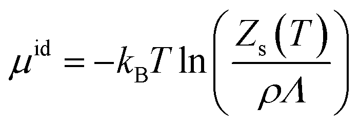 | (1) |
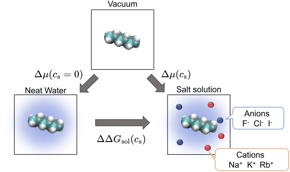 | ||
| Fig. 1 Thermodynamic cycle involving three states relating the transfer free energy of a solute from neat water to salt solutions (ΔΔGsol, horizontal equilibrium), the solvation free energy of the solute in neat water (Δμ(cs = 0), left vertical equilibrium), and the solvation free energy in salt solution (Δμ(cs), right vertical equilibrium). The transfer free energy is expressed by the solvation free energies according to eqn (2). | ||
ΔΔG(cs) is then written as
| ΔΔGsol(cs) = Δμ(cs) − Δμ(cs = 0), | (2) |
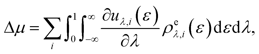
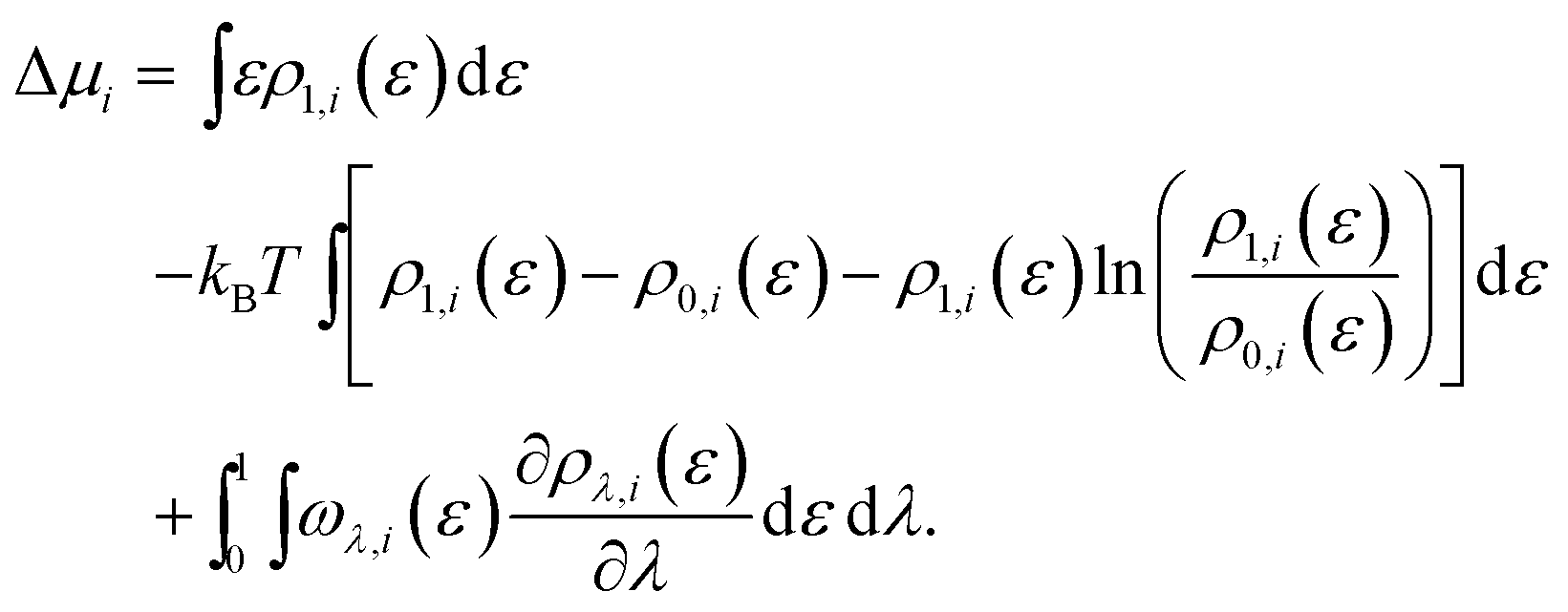
Computational methodologies revolving around (solvation) free-energy calculations have undergone tremendous development yielding a broad array of mainstream methods like the Widom insertion method,52 thermodynamic integration,53 the Bennett acceptance ratio method,54,55 and more.56 An alternative approach is the utilisation of the novel energy-representation theory of solvation.57–59 The method's strong appeal lies in its ability to decompose straightforwardly the solvation free energy into the contribution from each solvent species and further into the contributions from a variety of intermolecular-interaction components including the excluded-volume effect. This trait is particularly useful when studying multi-component liquids such as salt solutions, where the salt species are treated as solvents together with water. In fact, the separated contributions are often useful for physical interpretation and prediction, while they are not observable in general. A model of solvation then needs to be adopted to conduct the decomposition. As will be seen in Results & discussion section, the energy-representation formalism offers a framework for free-energy decomposition. The energy-representation theory rests upon the Kirkwood charging formula53 with the density distribution function being projected onto the solute–solvent pair-energy coordinate.57–59 For flexible solute molecules, the method relies on three systems simulated: the solute in the absence of solvent (referred to as vacuum system), the solute energetically decoupled from the solvent (referred to as the reference system), and the solute fully coupled to the solvent (referred to as the solution system). The details underlying the sampling of these systems are described in the following.
2.1 Molecular dynamics simulations
All-atom molecular dynamics simulations were conducted using the OpenMM60 (8.0.0) toolkit, modded with the MDTraj61 (1.9.7) package. For the reference and solution systems mentioned above, simulations in the isothermal-isobaric (NPT) ensemble were conducted using a combination of Langevin dynamics and Monte Carlo barostating. The temperature regulation employed the ‘middle discretisation’ Langevin leap-frog integrator scheme,62 with a target temperature of 298.15 K, a collision rate of 1.0 ps−1, and an integration time of 2 fs. The pressure was maintained using the Monte Carlo barostat,63,64 targeting a pressure of 1 bar. Isotropic volume perturbations were conducted every 25 steps, selecting the perturbation volume as a uniform random number between −1 and 1 scaled by a constant. This constant, updated during the simulation, ensured an acceptance rate of 50%.In this work, we examine the solvation of n-alcohols and n-alkanes from methane/methanol to n-hexane/n-hexanol in salt solutions with an alkali metal of Na+, K+, or Rb+ and a halogen anion of F−, Cl−, or I−. The OpenFF force field codename “Sage”65,66 (2.0) was employed for n-alcohols and n-alkanes, in combination with the OPC water model67 and Sengupta & Merz parameters68 for the cations and anions. Although Sage has been developed against the TIP3P69 water model, OPC was selected due to its excellent ability in reproducing bulk properties of water.67 To check the validity of our results, simulations were also conducted using a different set of force fields. GAFF70 (2.11) was employed for n-alcohols and n-alkanes, in combination with the SPC/E water model71,72 and alkali cations and halide anions by Heyda et al.,73 Dang,74 and Kalcher and Dzubiella.75 The results of these simulations are presented in the ESI section† named “Results of GAFF/SPCE/Heyda (GSH) Force Field”.76
Initial configurations were generated using Packmol77 (20.3.5) with the system geometry being cubic with a cell length of ∼67 Å. For the solution system, the MD cell contains 1 solute molecule (alcohol or alkane) and 10![[thin space (1/6-em)]](https://www.rsc.org/images/entities/char_2009.gif) 000 water molecules possibly with ions, and the numbers of the cation and anion are 0, 90, or 180 depending on the salt concentration of 0 M (water without ions), ∼0.5 M, and ∼1.0 M, respectively. For the reference systems, only water and salt were present in the same amount as in the solution systems. The initial configurations were minimised using the limited-memory BFGS optimisation algorithm78 until a tolerance of 10 kJ mol−1 has been reached. After the minimisation, the velocities were assigned according to the Maxwell–Boltzmann distribution at 298.15 K and the system was equilibrated for 1 ns at constant temperature and pressure.
000 water molecules possibly with ions, and the numbers of the cation and anion are 0, 90, or 180 depending on the salt concentration of 0 M (water without ions), ∼0.5 M, and ∼1.0 M, respectively. For the reference systems, only water and salt were present in the same amount as in the solution systems. The initial configurations were minimised using the limited-memory BFGS optimisation algorithm78 until a tolerance of 10 kJ mol−1 has been reached. After the minimisation, the velocities were assigned according to the Maxwell–Boltzmann distribution at 298.15 K and the system was equilibrated for 1 ns at constant temperature and pressure.
The reference systems were simulated for a total of 50 ns with the collection of configurations for statistical evaluation every 0.2 ps, while the solution systems were simulated for a total of 20 ns with a sampling interval of 0.2 ps. For both the reference and solution systems, the electrostatic potential energies and forces were evaluated using the Particle Mesh Ewald (PME) summation method79,80 using fifth-order B-splines, an error tolerance of 10−5, and a real-space cutoff of 1.2 nm. The Lennard–Jones interactions were subjected to switching functions81 using a fifth-order potential, with a switching range of 1.0–1.2 nm. The vacuum systems were simulated in the canonical ensemble (NVT) at 298.15 K, using the integration scheme mentioned at the beginning of this subsection at a time step of 1 fs. The Lennard–Jones energies and forces were evaluated with the same procedures as those for the reference and solution systems while the electrostatic interactions were handled in their generic 1/r form, without a cutoff. The vacuum simulations were run for 1 ns with sampling of solute structures every 0.01 ps.
For the calculation of radial distribution functions (RDFs) of the solute and solvent (water and ions) at a salt concentration of ∼1.0 M, 50 independent initial configurations were generated, following the procedures described above. Each replica was run for 20 ns, resulting in a cumulative simulation time of 1 μs across all replicas. RDFs were computed using the MDTraj61 (1.9.7) package.
2.2 Energy-representation theory of solvation
The energy-representation theory resolves around the utilisation of the pair-energy coordinate between the solute and the solvent as a projection function for the ensemble-averaged correlation functions.57 The instantaneous pair-interaction energy distribution for solvent species i, , is obtained at any given configuration by the definition of
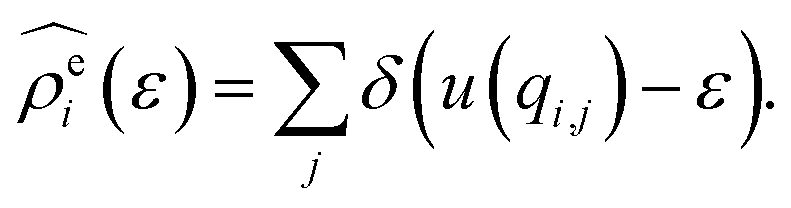 | (3) |
 | (4) |
 | (5) |
 | (6) |
For the calculation of solvation free energies, the ERmod software83 (0.3.7) has been utilised. Long-range dispersion correction was added to capture the contribution from Lennard–Jones interactions beyond the cutoff distance.87 To obtain the pair-energy distributions at λ = 0, 200 insertions of the solute were performed at random positions and orientations into each reference configuration sampled. Error estimation of the solvation free energies was done using block averaging with the reference and solution trajectories divided into 5 and 10 blocks, respectively.
3 Results & discussion
3.1 Quantifying salts' effects on the solvation: Setschenow coefficients
The Setschenow equation asserts that the transfer free energy from neat water to salt solution ΔΔGsol(cs) is linearly proportional to the salt concentration cs43,44,88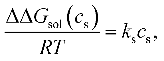 | (7) |
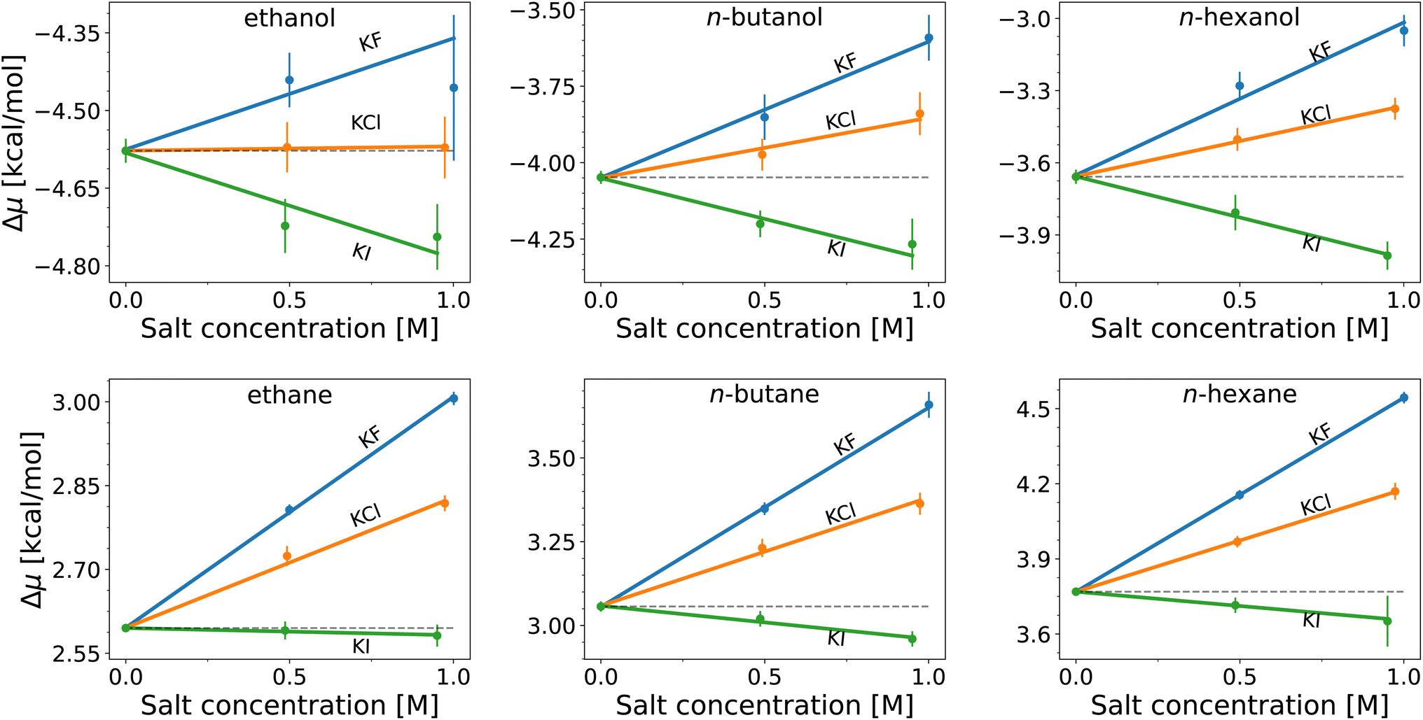 | ||
| Fig. 2 Solvation free energies, Δμ, of n-alcohols (top) and n-alkanes (bottom) as functions of potassium salt concentration, with the corresponding anions F− (blue), Cl− (orange), and I− (green). The lines are the best fits using the common value in neat water (zero concentration of the salt) for each solute. | ||
The hydration free energies (equal to the vertical intercept of Fig. 2, with numerical values in Table S1†) of the n-alcohols and n-alkanes are in agreement with experimental data89 with overestimation by ≲1 kcal mol−1 (smaller deviations for shorter chains). When salts are added, the solvation free energy changes linearly with the salt concentration for both the n-alcohols and n-alkanes, with the slope being proportional to the Setschenow coefficient according to eqn (7). According to Fig. 2, the sign of the Setschenow coefficient shows KF and KCl to salt-out, while KI acts to salt-in. The Hofmeister series is observed since the Setschenow coefficient is in the order of I− < Cl− < F− at fixed cation of K+. The points in Fig. 2 are more scattered for the n-alcohols than for the n-alkanes, and the plot for ethanol involves large error bars. This is an issue of sampling, and as described in the ESI with respect to Fig. S1 and S2,† the alcohol–ion interactions are slowly converging. The trend for the Setschenow coefficients is in qualitative agreement with experimental observations, with KF and KCl salting-out both the n-alcohols and n-alkanes.90,91 For KI, it is noted for the force field employed for Fig. 2 that the salt is salting-in the n-alcohols and marginally salting-in the n-alkanes.
To investigate the relative importance of the cations and anions, the Setschenow coefficients for all salt combinations are illustrated in Fig. 3 for n-hexanol and n-hexane. It is observed that the effect of changing the anion species dominates over that of the cation for the Setschenow coefficient. A similar observation has been done for caffeine, revealing that the anion effect is primary in the salt effect on the solvation.44 From here on out, we fix the cation to potassium when the decomposed contributions from cations and anions are discussed, while correlations with the variation of salts are examined over all the combinations of the cations and anions.
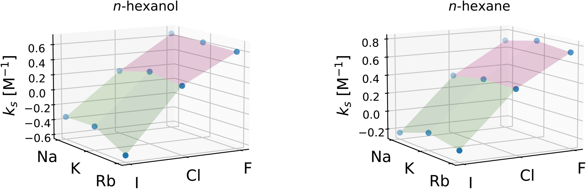 | ||
| Fig. 3 Setschenow coefficients, ks, for n-hexanol (left) and n-hexane (right) for all combinations of the cations: Na+, K+, and Rb+ and anions: F−, Cl−, and I−. ks are visualised as points, and the planes connecting adjacent points have been added for guidance. | ||
3.2 Cation–anion contrast in n-alcohol and n-alkane solvation
To gain mechanistic insights into the roles of the cation, anion, and water species in the solvation of the n-alcohols and n-alkanes, the solvation free energy Δμ has been decomposed into the contributions from the solvent species present in the system. Within the framework of the energy-representation theory, we can write Δμ as| Δμ = Δμself + Δμcation + Δμanion + Δμwater | (8) |
 | (9) |
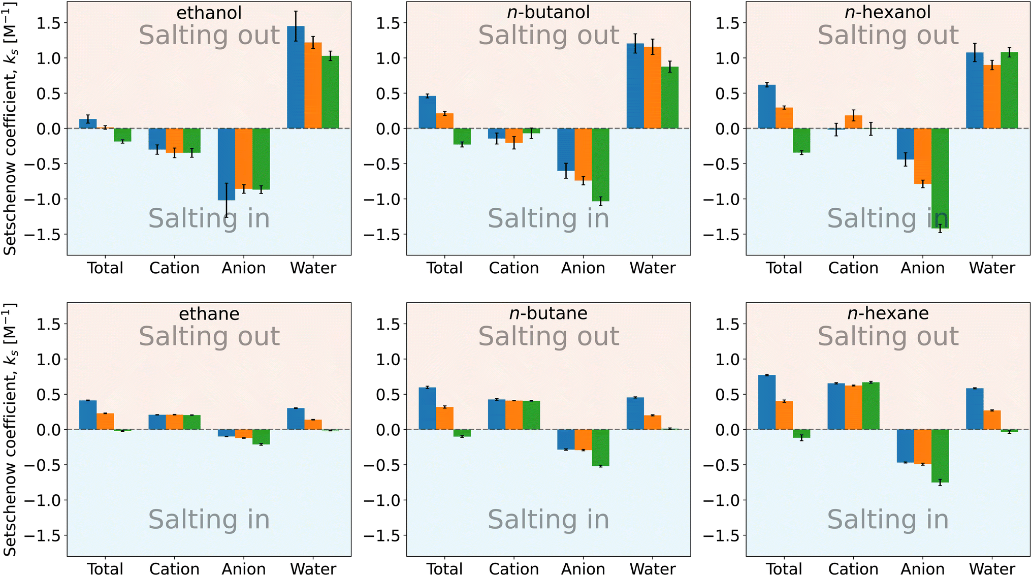 | ||
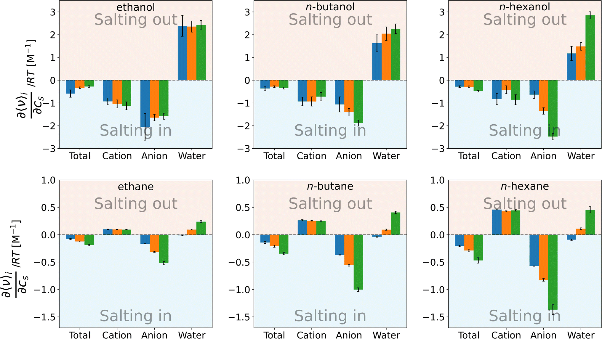
| Fig. 4 Setschenow coefficient, ks, and the contributions from the solvent species, namely cations, anions, and water, for n-alcohols (top) and n-alkanes (bottom) with potassium as the cation and F− (blue), Cl− (orange), and I− (green) as the anions. The cation, anion, and water contributions correspond to the first, second, and third terms of eqn (9). The self-energy correction was found not to vary with the salt concentration. The error bars shown report the 95% confidence interval as determined by non-parametric bootstrapping92 (N = 105) assuming the individual solvent contributions to vary linearly. | ||
For n-alcohols (Fig. 4, top row), the cations yield a negative or marginal contribution to the Setschenow coefficients, the anions provide a negative contribution, and the water contributions are positive. The contribution of cation (the cation is fixed to potassium) is weakly dependent on the corresponding anion, which is considered to reflect the full dissociation of the salt. The magnitude of the cation contribution becomes smaller with the chain length of the n-alcohols. The relative strengths of the anion contributions vary with the alcohol species examined. The anions act to salt-in the alcohols. Among the cation, anion, and water, the contribution is the most favourable from the anion, and in Fig. 4, the ordering of F− < Cl− < I− for the tendency of salting-in is observed for n-butanol and n-hexanol in agreement with the Hofmeister series. The water contribution is positive, showing its role to reduce the solubility when the transfer from neat water to the salt solution is concerned.
For n-alkane solvation (Fig. 4, bottom row), the cations and anions play contrasting roles to modulate the solubility. The former yield a positive contribution to the Setschenow coefficient with the negative or marginal contribution from the anions. The cation contribution is independent of the accompanying anion as observed for the alcohol solutes. The anion contrbution depends on the salt species, with the weak correspondence to the anion size. As for the water contribution, KF > KCl > KI is seen, where the KF values are positive and the KI values are negative or maginal. When the alkyl chain is elongated, the general tendency is that both the cation and anion contributions increase in magnitude, with the enhancement of the water contribution.
The parallelism and contrast to the previous results for caffeine44 are as follows. For all the solutes examined, the Hofmeister series holds for the Setschenow coefficients (total values in Fig. 4). The differences are observed for the separated contributions from cations and anions. For caffeine, the cations act to salt-in and the anions to salt-out, while for the n-alkanes, the opposite holds. For the n-alcohols, the anions act to salt-in with favourable or marginal contributions from the cations as observed in Fig. 4. The water contribution is positive for most of caffeine, n-alcohols, and n-alkanes, showing that water often becomes less favourable for a solute when a salt is added. To see the effects of the cations, anions, and water more closely, we will further examine the solvent-species contribution to the Setschenow coefficients.
3.3 Roles of the solute–solvent interactions
Within the framework of the energy-representation theory of solvation, the contribution to the solvation free energy from a single solvent species (see eqn (8)) can be written as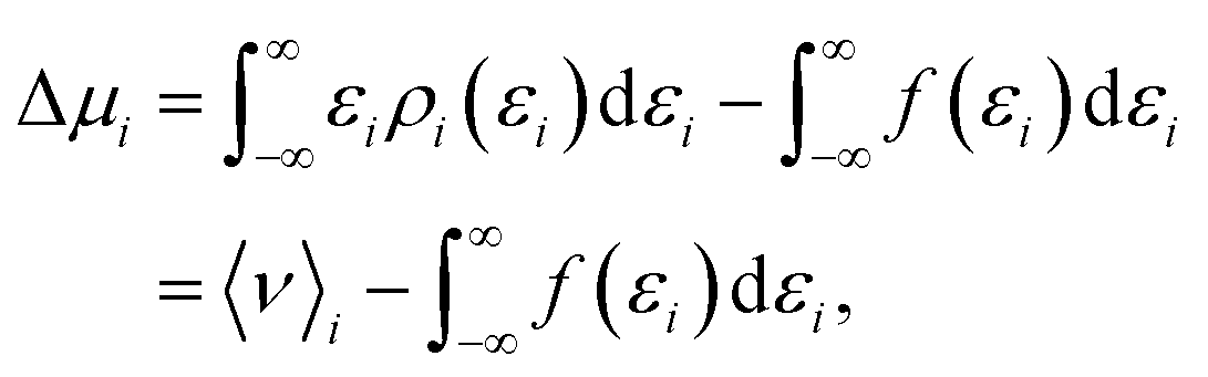 | (10) |
 | (11) |
To see the effect of direct solute–solvent interactions on the Setschenow coefficient, Fig. 5 shows the first term of eqn (11). For all the solutes in Fig. 5, the change in the total interaction energy between the solute and solvent is favourable (negative) upon addition of the salt and acts to increase the solubility. The separated contribution from cation is in contrast between the n-alcohols and n-alkanes, and it is negative for the former and positive for the latter. The negative values from the cation stem from its ability to interact with the hydroxyl groups of the n-alcohols. The n-alkane solutes have weakly positive charges on the hydrogens, and this leads to the positive interaction energies. With the anion contribution, the n-alkanes are salted-in with the ranking of I− > Cl− > F−. This ranking is further valid for n-hexanol, which has a long alkyl chain. It has been noted that weakly hydrated anions preferentially accumulate near hydrophobic surfaces.10,18,93 It is then expected that the water molecules around a hydrophobic motif will be displaced to accommodate the anion. The correlation between the solute–anion interaction energy and the Setschenow coefficient is indeed positive when the salt species is varied and the alkane solute is fixed (Fig. S3†), while an anti-correlation is seen for the salt-induced change in the solute–water interaction (Fig. S4†). The direct interaction of the alkane solute with an anion that salts-in more strongly is more favourable at the energetic expense of water.
 | ||
| Fig. 5 Species decomposition of the contributions to the Setschenow coefficient from the direct interaction energies between the solute and solvent for n-alcohols (top) and n-alkanes (bottom), with potassium as the cation and F− (blue), Cl− (orange), and I− (green) as the anions. The error bars shown report the 95% confidence interval determined by non-parametric bootstrapping92 (N = 105) assuming the individual solvent contributions to vary linearly. | ||
To discuss the solvation structures underlying the energetics, we illustrate the radial distribution functions (RDFs) of n-hexane in the 1 M mixtures of water and potassium salts in Fig. 6. The RDFs with the anions are compared in Fig. 6A, and iodide ions are observed to accumulate closely to the n-hexane. The exclusion from the solute surface is more evident in the order of F− > Cl− > I−. Fig. 6B depicts the RDFs for potassium. The cation is excluded from the surface of n-hexane regardless of the anion species and exhibits an increased extent of presence in the order of I− > Cl− > F−. This is considered to reflect the electrostatic attraction between the cation and anion. When the anion is accumulated more strongly around the solute, K+ comes more closely to the solute surface. The above features of RDF correspond to the energetic observations for 〈ν〉 in Fig. 5. Among the three anions of F−,Cl−, and I−, for example, the direct interaction with the solute n-hexane in Fig. 5 is more favourable in the order of I− > Cl− > F−, with the same ordering of accumulation tendency around the solute.
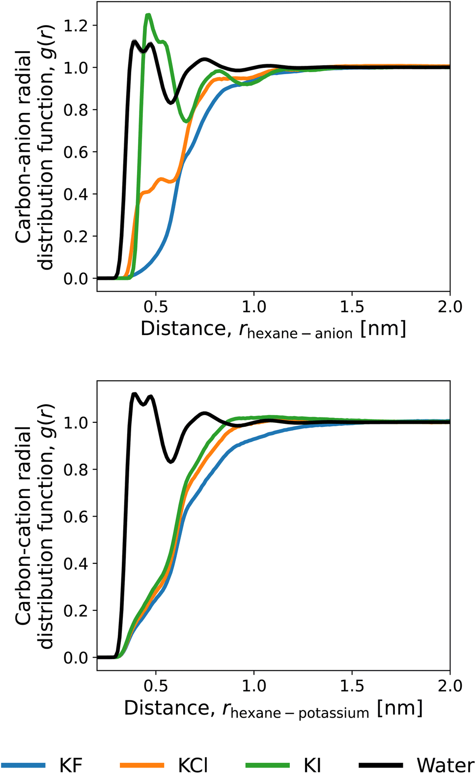 | ||
| Fig. 6 Radial distribution functions (RDFs) in the ∼1 M salt solutions of the carbon of n-hexane with potassium as the cation and F− (blue), Cl− (orange), and I− (green) as the anions. The distributions of water oxygen are also shown (black). The water RDF is insensitive to the choice of the salt, and its differences among the salt species are not appreciable within the resolution of the figure. The RDFs for the 6 carbon atoms are averaged in this figure. | ||
The Kirkwood–Buff theory is another route to addressing salt-induced changes in solubilities.94 As pointed out by Smith and Mazo and Katsuto et al.,95,96 though, the Kirkwood–Buff integral of the monovalent cation with the solute is equal to that for the monovalent anion even when the short-range features of RDF are different between the cation and anion. This is due to the 1:1 dissociation of the salt, and according to Fig. 6, the long-distance region of RDF needs to be treated at high precision to attain the equality. We do not address the Kirkwood–Buff integrals in this work since they did not converge within our computational setups.
To investigate the effect of solvent reorganisation together with the interaction energy (i.e. going from an energy to a free energy), we can choose the integration limits of eqn (10) to the energy domain of a characteristic interaction. When the upper limit of integration in eqn (11) is set to εmax and it is much larger than RT, the average solute–solvent interaction energy (the first integral in the first line of eqn (10)) becomes invariant with εmax (ρi(εi) vanishes when εi > εmax), while f(εi) for εi > εmax instead will reflect the effect of excluded volume. We then define the following energy domains:
• −∞ < εi < εmax: effects of interactions such as hydrogen bonding and dispersion and associated solvent-reorganisation effects.
• εmax < εi < ∞: effects of solvent displacement for cavity formation (excluded-volume effects).
The choice of εmax has been done from the maximum pair energy between the solute and solvent in the simulations of the solutions. When scanned over all salts, salt concentrations, and solutes, the largest pair energy observed has been 14.6 kcal mol−1 and thus εmax = 15 kcal mol−1 has been set as an appropriate choice. We note that the largest energy observed in a molecular simulation is related to the sampling of rare events and therefore subject to change, however, the results and conclusions in the following are not altered with any (reasonable) choice of εmax.
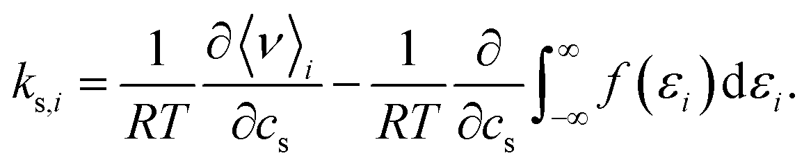
In order to quantify the effect of the solvent reorganisation on the Setschenow coefficient, we introduce the partial contribution to eqn (11) as
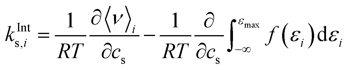 | (12) |
3.4 Effect of excluded volume
The effect of excluded volume can be addressed on the basis of eqn (11), and the contribution from solvent species i (i is cation, anion, or water) to the excluded-volume component in the Setschenow coefficient, kEVs,i, is given by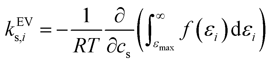 | (13) |
 | ||
| Fig. 7 Correlation between the total Setschenow coefficient and the excluded-volume component obtained from integration over the high-energy domain. Data are shown for all the combinations of cations (Na+, K+, and Rb+) and anions (F−, Cl−, and I−). The data symbols are shaped depending on the cation species: Na+ (triangle), K+ (circle), and Rb+ (inverse triangle) and coloured depending on the anion species: F− (blue), Cl− (orange), and I− (green). The solute refers to ethanol and ethane with Ncarbon = 2, to n-butanol and n-butane with Ncarbon = 4, and to n-hexanol and n-hexane with Ncarbon = 6. The symbols are filled and open for the n-alcohols and n-alkanes, respectively. | ||
They are well correlated when the solute is fixed and the salts are varied. In Fig. 7, all the combinations of cations (Na+, K+, and Rb+) and anions (F−, Cl−, and I−) are plotted for each solute and the data are clustered according to the anion species. This shows the dominance of the anion effect upon variation of the salt species, with F− > Cl− > I− for both the Setschenow coefficient and the excluded-volume component. Accordingly, the effects of salting-in and salting-out can be described by the free-energy penalty of creating a cavity. To investigate this idea further, the role of each of the cation, anion, and water in the excluded-volume component is examined. The separated contributions are visualised in Fig. 8.
 | ||
| Fig. 8 Species decomposition of the excluded-volume component in the Setschenow coefficient for n-alcohols (top) and n-alkanes (bottom) with potassium as the cation and F− (blue), Cl− (orange), and I− (green) as the anions. The error bars shown report the 95% confidence interval determined by non-parametric bootstrapping92 (N = 105) assuming the individual solvent contributions to vary linearly. | ||
The cation and anion contributions are positive for all the combinations of solute and salt. For the cations, the excluded-volume component is independent of the accompanying anion, which is expected since the excluded-volume effect is caused by the overlap of the solute and solvent upon insertion of the solute into the reference system. For the anions, the series of F− < Cl− < I− is observed, reflecting the ionic radii of the halogens. With the increase of the solute size, the excluded-volume component becomes larger since the overlap between the solute and salt enhances with the solute size. It should be noted, though, that when the solute is fixed and the salt species is varied, either the cation or anion contribution to the excluded-volume component in the Setschenow coefficient is not correlated to the total value of the excluded-volume component. This implies the importance of the water contribution.
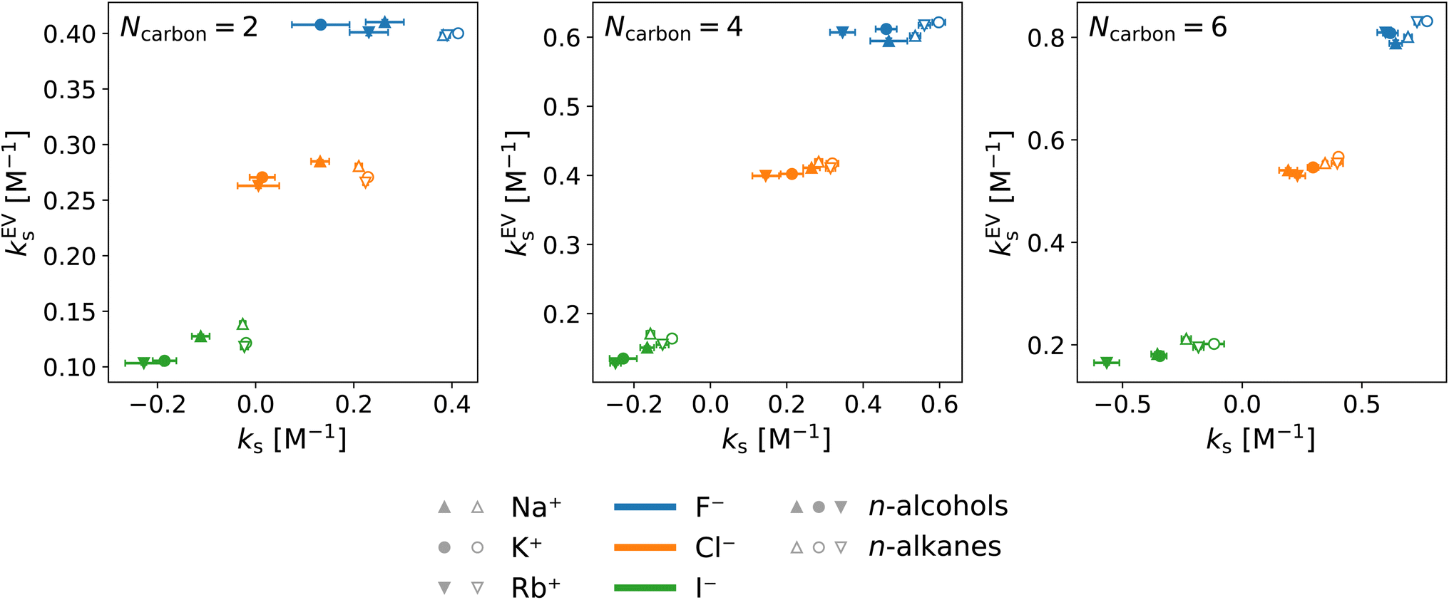
Fig. 8 and 9 show that the water contribution to the excluded-volume component correlates to the total in the dependence on the salt species. Note that the water contribution refers here to the difference in the excluded-volume effect between the salt solution and neat water. It is positive with KF, small in magnitude with KCl, and negative with KI for all the n-alcohol and n-alkane solutes examined. The salt-induced changes in the free-energy penalties of cavity formation are more favourable (negative) for larger anions. This is related to the changes in the water density, as will be discussed later. It is seen in Fig. 9, furthermore, that both the total and water contributions are clustered according to the anion species and are close to each other between the n-alcohol and n-alkane when the numbers of carbon atoms (Ncarbon) are the same. The slopes of the solid lines in Fig. 9 are also similar over Ncarbon = 2, 4, and 6. The excluded-volume effect is close between the alcohol and alkane with similar sizes and appears in the dependence on the salt species through the water contribution.
 | ||
| Fig. 9 Correlation between the total excluded-volume component in the Setschenow coefficient and the water contribution. Data are shown for all the combinations of cations (Na+, K+, and Rb+) and anions (F−, Cl−, and I−). The solid lines connect the data with the same length of the alkyl chain (Ncarbon) and varied species of salts. The dashed lines are for fixed salts with varied solutes. The solute refers to ethanol and ethane with Ncarbon = 2, to n-butanol and n-butane with Ncarbon = 4, and to n-hexanol and n-hexane with Ncarbon = 6. The data symbols are shaped depending on the cation species: Na+ (triangle), K+ (circle), and Rb+ (inverse triangle) and coloured depending on the anion species: F− (blue), Cl− (orange), and I− (green). The symbols are filled and open for the n-alcohols and n-alkanes, respectively. | ||
For the variation of the solute at fixed salt, the correlations between the total excluded-volume component and the water contribution to it are depicted in Fig. 9 with dashed lines. All the lines pass near the origin. Accordingly, both the total and water contributions to the excluded-volume component grow in magnitude with the solute size and the water contribution is negative with large anions. The negative growth of the water contribution with the solute size reflects the observation in the next paragraph that the water density decreases with addition of the iodide salts.
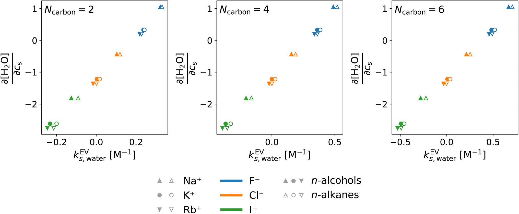
In the above, the importance of the water contribution was seen in the excluded-volume component in the Setschenow coefficient, and in ref. 44, it was observed for the caffeine solute that the water contribution is correlated to the change in the water density upon introduction of the solute. Fig. 10 provides correlation plots between the water contribution to the excluded-volume component and the response of the water density to the addition of the salt  . The addition of KI or KCl salt reduces the density (molarity) of water, while KF increases the water density. The salt's effect on the water density is parallel to the size of the ion, and in Fig. 10, the water contribution to the excluded-volume component is well correlated to the change in the water density. This observation holds over all the n-alcohol and n-alkane solutes as well as caffeine.44 The water contribution to the excluded-volume component is smaller when the salt reduces the water density, and vice versa. The line connecting
  and kEVs,water does not pass through the origin. kEVs,water ≈ 0 corresponds to
  , which was also observed for caffeine in salt solutions, despite employing a different water model, solute, and ion force fields. The importance of the excluded-volume effect was pointed out for salt effects on the solubilities of small solutes with semi-explicit methods.41–43,97,98 It was seen that although the electrostatic interactions act to increase the solubilities,43 the excluded-volume component governs the salt-induced changes in the solvation free energies. This is in agreement with our results, while we employed a different model of solvation and maintain an all-atom representation throughout the computation.
 | ||
| Fig. 10 Correlation between the derivative of the water molarity with respect to the salt concentration and the water contribution to the excluded-volume component in the Setschenow coefficient. Data are shown for all the combinations of cations (Na+, K+, and Rb+) and anions (F−, Cl−, and I−). The data symbols are shaped depending on the cation species: Na+ (triangle), K+ (circle), and Rb+ (inverse triangle) and coloured depending on the anion species: F− (blue), Cl− (orange), and I− (green). The solute refers to ethanol and ethane with Ncarbon = 2, to n-butanol and n-butane with Ncarbon = 4, and to n-hexanol and n-hexane with Ncarbon = 6. The symbols are filled and open for the n-alcohols and n-alkanes, respectively. | ||
4 Conclusions
We have addressed the role of salt on the solvation of n-alcohols and n-alkanes by using all-atom MD simulation and the energy-representation theory of solvation. It has been found, in agreement with the general consensus on ion-specific effects, that the anion species govern the ranking of the salt-species dependence of the Setschenow coefficient. The free-energy decomposition has then been conducted to elucidate the roles of the cation, anion, and water and of the direct solute–solvent interactions and the excluded-volume component by focusing on the correlations with the Setschenow coefficient. When the salt species is varied with a fixed solute, the Setschenow coefficient is correlated to the direct interaction between the solute and anion for the alkanes and to the excluded-volume component for all the solutes examined. The favourable interactions with large anions like iodide corresponds to its accumulation around hydrophobic groups and brings the salting-in effect. The dependence of the excluded-volume component on the salt species is parallel to the water contribution to it, which is in turn correlated to the change of the water density upon addition of the salt. The density change is a volumetric aspect of the salt-induced effect, and on the basis of correlation analyses, the role of the excluded-volume component has been pointed out in the salts' effects on the Setschenow coefficient.It has been observed through correlation analyses that the excluded-volume effect can describe the salt-induced changes in the solubility. Although the separated components in the free energy are not observable in general, they may be physically appealing and suitable for prediction. The excluded-volume effect is a notable example, and since it is further correlated to the salt-induced change in the water density, a predictive discussion of salt-specific effects is possible with the volumetric term.
Data availability
Software, simulations, and analysis for reproduction have been deposited at Zenodo for the Sage/OPC/Sengupta & Merz Force Field (DOI: 10.5281/zenodo.8307836) and for the GAFF/SPCE/Heyda force field (DOI: 10.5281/zenodo.10046776).Author contributions
The study was designed and conceptualized by SHH and NM. Simulations and analyse were performed by SHH and DL. The results were discussed and interpreted by all the authors. The manuscript was written by SHH and NM and advanced by SHH, KK, and NM.Conflicts of interest
There are no conflicts to declare.Acknowledgements
SHH is grateful to the Postdoctoral Fellowship for Research in Japan (No. 22F21756) from the Japan Society for the Promotion of Science. This work is supported by the Grants-in-Aid for Scientific Research (No. JP22KF0240, JP23H02622, and JP23H01924) from the Japan Society for the Promotion of Science and by the Fugaku Supercomputer Project (No. JPMXP1020230325 and JPMXP1020230327) and the Data-Driven Material Research Project (No. JPMXP1122714694) from the Ministry of Education, Culture, Sports, Science, and Technology. The simulations were conducted using Cygnus at Tsukuba University, TSUBAME3.0 at Tokyo Institute of Technology, kugui at University of Tokyo, flow at Nagoya University, ITO at Kyushu University, and Fugaku at RIKEN Advanced Institute for Computational Science through the HPCI System Research Project (Project IDs: hp230101, hp230158, hp230205, and hp230212).References
- A. Ben-Naim, K.-L. Ting and R. L. Jernigan, Biopolymers, 1989, 28, 1309–1325 CrossRef CAS.
- A. Ben-Naim, K.-L. Ting and R. L. Jernigan, Biopolymers, 1989, 28, 1327–1337 CrossRef CAS PubMed.
- J. Hernández-Lima, K. Ramírez-Gualito, B. Quiroz-García, A. L. Silva-Portillo, E. Carrillo-Nava and F. Cortés-Guzmán, Front. Chem., 2022, 10, 1012769 CrossRef PubMed.
- W. Kauzmann, in Advances in Protein Chemistry, Elsevier, 1959, pp. 1–63 Search PubMed.
- L. R. Pratt and D. Chandler, J. Chem. Phys., 1977, 67, 3683–3704 CrossRef CAS.
- C. Tanford, Protein Sci., 1997, 6, 1358–1366 CrossRef CAS PubMed.
- S. Otto and J. B. F. N. Engberts, Org. Biomol. Chem., 2003, 1, 2809 RSC.
- R. Patil, S. Das, A. Stanley, L. Yadav, A. Sudhakar and A. K. Varma, PLoS One, 2010, 5, e12029 CrossRef.
- S. G. Krimmer, J. Cramer, J. Schiebel, A. Heine and G. Klebe, J. Am. Chem. Soc., 2017, 139, 10419–10431 CrossRef CAS PubMed.
- H. I. Okur, J. Hladílková, K. B. Rembert, Y. Cho, J. Heyda, J. Dzubiella, P. S. Cremer and P. Jungwirth, J. Phys. Chem. B, 2017, 121, 1997–2014 CrossRef CAS.
- B. Kang, H. Tang, Z. Zhao and S. Song, ACS Omega, 2020, 5, 6229–6239 CrossRef CAS.
- E. E. Bruce, H. I. Okur, S. Stegmaier, C. I. Drexler, B. A. Rogers, N. F. A. van der Vegt, S. Roke and P. S. Cremer, J. Am. Chem. Soc., 2020, 142, 19094–19100 CrossRef CAS.
- F. A. Long and W. F. McDevit, Chem. Rev., 1952, 51, 119–169 CrossRef CAS.
- F. Hofmeister, Arch. Exp. Pathol. Pharmakol., 1888, 24, 247–260 CrossRef.
- W. Kunz, J. Henle and B. Ninham, Curr. Opin. Colloid Interface Sci., 2004, 9, 19–37 CrossRef CAS.
- B. A. Deyerle and Y. Zhang, Langmuir, 2011, 27, 9203–9210 CrossRef CAS PubMed.
- O. A. Francisco, H. M. Glor and M. Khajehpour, ChemPhysChem, 2020, 21, 484–493 CrossRef CAS PubMed.
- B. A. Rogers, H. I. Okur, C. Yan, T. Yang, J. Heyda and P. S. Cremer, Nat. Chem., 2021, 14, 40–45 CrossRef.
- G. Jones and M. Dole, J. Am. Chem. Soc., 1929, 51, 2950–2964 CrossRef CAS.
- O. M. Cabarcos, C. J. Weinheimer, J. M. Lisy and S. S. Xantheas, J. Chem. Phys., 1999, 110, 5–8 CrossRef CAS.
- I. A. Topol, G. J. Tawa, S. K. Burt and A. A. Rashin, J. Chem. Phys., 1999, 111, 10998–11014 CrossRef CAS.
- J. Kim, H. M. Lee, S. B. Suh, D. Majumdar and K. S. Kim, J. Chem. Phys., 2000, 113, 5259–5272 CrossRef CAS.
- A. W. Omta, M. F. Kropman, S. Woutersen and H. J. Bakker, Science, 2003, 301, 347–349 CrossRef CAS PubMed.
- L.-Å. Näslund, D. C. Edwards, P. Wernet, U. Bergmann, H. Ogasawara, L. G. M. Pettersson, S. Myneni and A. Nilsson, J. Phys. Chem. A, 2005, 109, 5995–6002 CrossRef.
- D. A. Schmidt, R. Scipioni and M. Boero, J. Phys. Chem. A, 2009, 113, 7725–7729 CrossRef CAS.
- Y. Marcus, Chem. Rev., 2009, 109, 1346–1370 CrossRef CAS PubMed.
- P. Gallo, D. Corradini and M. Rovere, Phys. Chem. Chem. Phys., 2011, 13, 19814 RSC.
- N. Galamba, J. Phys. Chem. B, 2012, 116, 5242–5250 CrossRef CAS PubMed.
- I. Juurinen, T. Pylkkänen, K. O. Ruotsalainen, C. J. Sahle, G. Monaco, K. Hämäläinen, S. Huotari and M. Hakala, J. Phys. Chem. B, 2013, 117, 16506–16511 CrossRef CAS.
- G. Stirnemann, E. Wernersson, P. Jungwirth and D. Laage, J. Am. Chem. Soc., 2013, 135, 11824–11831 CrossRef CAS.
- M. Kondoh, Y. Ohshima and M. Tsubouchi, Chem. Phys. Lett., 2014, 591, 317–322 CrossRef CAS.
- Y. Chen, H. I. Okur, N. Gomopoulos, C. Macias-Romero, P. S. Cremer, P. B. Petersen, G. Tocci, D. M. Wilkins, C. Liang, M. Ceriotti and S. Roke, Sci. Adv., 2016, 2, e1501891 CrossRef PubMed.
- A. P. Gaiduk and G. Galli, J. Phys. Chem. Lett., 2017, 8, 1496–1502 CrossRef CAS PubMed.
- P. Luo, Y. Zhai, E. Senses, E. Mamontov, G. Xu, Y Z and A. Faraone, J. Phys. Chem. Lett., 2020, 11, 8970–8975 CrossRef CAS.
- S. Gómez, N. Rojas-Valencia, S. A. Gómez, C. Cappelli, G. Merino and A. Restrepo, Chem. Sci., 2021, 12, 9233–9245 RSC.
- C. Zhang, S. Yue, A. Z. Panagiotopoulos, M. L. Klein and X. Wu, Nat. Commun., 2022, 13, 822 CrossRef CAS PubMed.
- T. G. Pedersen and A. Hvidt, Carlsberg Res. Commun., 1985, 50, 193–198 CrossRef.
- Y. Marcus, Chem. Rev., 2011, 111, 2761–2783 CrossRef CAS.
- V. Mazzini and V. S. J. Craig, Chem. Sci., 2017, 8, 7052–7065 RSC.
- M. Kinoshita, Biophys. Rev., 2013, 5, 283–293 CrossRef CAS.
- G. Graziano, J. Chem. Phys., 2008, 129, 084506 CrossRef.
- S. Murakami, T. Hayashi and M. Kinoshita, J. Chem. Phys., 2017, 146, 055102 CrossRef PubMed.
- L. Li, C. J. Fennell and K. A. Dill, J. Chem. Phys., 2014, 141, 22D518 CrossRef PubMed.
- S. Hervø-Hansen, J. Heyda, M. Lund and N. Matubayasi, Phys. Chem. Chem. Phys., 2022, 24, 3238–3249 RSC.
- K. D. Collins, Proc. Natl. Acad. Sci. U. S. A., 1995, 92, 5553–5557 CrossRef CAS PubMed.
- R. Zangi, M. Hagen and B. J. Berne, J. Am. Chem. Soc., 2007, 129, 4678–4686 CrossRef CAS.
- M. Lund, R. Vácha and P. Jungwirth, Langmuir, 2008, 24, 3387–3391 CrossRef CAS.
- M. Lund, L. Vrbka and P. Jungwirth, J. Am. Chem. Soc., 2008, 130, 11582–11583 CrossRef CAS.
- Y. Zhang and P. S. Cremer, Annu. Rev. Phys. Chem., 2010, 61, 63–83 CrossRef CAS.
- K. B. Rembert, J. Paterová, J. Heyda, C. Hilty, P. Jungwirth and P. S. Cremer, J. Am. Chem. Soc., 2012, 134, 10039–10046 CrossRef CAS.
- B. A. Rogers, T. S. Thompson and Y. Zhang, J. Phys. Chem. B, 2016, 120, 12596–12603 CrossRef CAS.
- B. Widom, J. Chem. Phys., 1963, 39, 2808–2812 CrossRef CAS.
- J. G. Kirkwood, J. Chem. Phys., 1935, 3, 300–313 CrossRef CAS.
- C. H. Bennett, J. Comput. Phys., 1976, 22, 245–268 CrossRef.
- M. R. Shirts and J. D. Chodera, J. Chem. Phys., 2008, 129, 124105 CrossRef PubMed.
- R. E. Skyner, J. L. McDonagh, C. R. Groom, T. van Mourik and J. B. O. Mitchell, Phys. Chem. Chem. Phys., 2015, 17, 6174–6191 RSC.
- N. Matubayasi and M. Nakahara, J. Chem. Phys., 2000, 113, 6070–6081 CrossRef CAS.
- N. Matubayasi and M. Nakahara, J. Chem. Phys., 2002, 117, 3605–3616 CrossRef CAS.
- N. Matubayasi and M. Nakahara, J. Chem. Phys., 2003, 119, 9686–9702 CrossRef CAS.
- P. Eastman, J. Swails, J. D. Chodera, R. T. McGibbon, Y. Zhao, K. A. Beauchamp, L.-P. Wang, A. C. Simmonett, M. P. Harrigan, C. D. Stern, R. P. Wiewiora, B. R. Brooks and V. S. Pande, PLoS Comput. Biol., 2017, 13, e1005659 CrossRef PubMed.
- R. T. McGibbon, K. A. Beauchamp, M. P. Harrigan, C. Klein, J. M. Swails, C. X. Hernández, C. R. Schwantes, L.-P. Wang, T. J. Lane and V. S. Pande, Biophys. J., 2015, 109, 1528–1532 CrossRef CAS PubMed.
- Z. Zhang, X. Liu, K. Yan, M. E. Tuckerman and J. Liu, J. Phys. Chem. A, 2019, 123, 6056–6079 CrossRef CAS.
- K.-H. Chow and D. M. Ferguson, Comput. Phys. Commun., 1995, 91, 283–289 CrossRef CAS.
- J. Åqvist, P. Wennerström, M. Nervall, S. Bjelic and B. O. Brandsdal, Chem. Phys. Lett., 2004, 384, 288–294 CrossRef.
- Y. Qiu, D. G. A. Smith, S. Boothroyd, H. Jang, D. F. Hahn, J. Wagner, C. C. Bannan, T. Gokey, V. T. Lim, C. D. Stern, A. Rizzi, B. Tjanaka, G. Tresadern, X. Lucas, M. R. Shirts, M. K. Gilson, J. D. Chodera, C. I. Bayly, D. L. Mobley and L.-P. Wang, J. Chem. Theory Comput., 2021, 17, 6262–6280 CrossRef CAS.
- J. Wagner, M. Thompson, D. Dotson, S. B. Hyejang and J. Rodríguez-Guerra, Openforcefield/openff-forcefields: Version 2.0.0 ”Sage”, 2021, https://zenodo.org/record/5214478 Search PubMed.
- S. Izadi, R. Anandakrishnan and A. V. Onufriev, J. Phys. Chem. Lett., 2014, 5, 3863–3871 CrossRef CAS PubMed.
- A. Sengupta, Z. Li, L. F. Song, P. Li and K. M. Merz, J. Chem. Inf. Model., 2021, 61, 869–880 CrossRef CAS.
- W. L. Jorgensen, J. Chandrasekhar, J. D. Madura, R. W. Impey and M. L. Klein, J. Chem. Phys., 1983, 79, 926–935 CrossRef CAS.
- J. Wang, R. M. Wolf, J. W. Caldwell, P. A. Kollman and D. A. Case, J. Comput. Chem., 2004, 25, 1157–1174 CrossRef CAS.
- H. J. C. Berendsen, J. R. Grigera and T. P. Straatsma, J. Phys. Chem., 1987, 91, 6269–6271 CrossRef CAS.
- S. Chatterjee, P. G. Debenedetti, F. H. Stillinger and R. M. Lynden-Bell, J. Chem. Phys., 2008, 128, 124511 CrossRef.
- J. Heyda, J. C. Vincent, D. J. Tobias, J. Dzubiella and P. Jungwirth, J. Phys. Chem. B, 2009, 114, 1213–1220 CrossRef.
- L. X. Dang, J. Phys. Chem. B, 1999, 103, 8195–8200 CrossRef CAS.
- I. Kalcher and J. Dzubiella, J. Chem. Phys., 2009, 130, 134507 CrossRef.
- S. Hervø-Hansen, Electronic notebook: Free-energy decomposition of salt effects on the solubilities of small molecules and the role of excluded-volume effects (GAFF/SPCE/Heyda force field), 2023, https://zenodo.org/doi/10.5281/zenodo.10046776.
- L. Martínez, R. Andrade, E. G. Birgin and J. M. Martínez, J. Comput. Chem., 2009, 30, 2157–2164 CrossRef PubMed.
- D. C. Liu and J. Nocedal, Math. Program., 1989, 45, 503–528 CrossRef.
- T. Darden, D. York and L. Pedersen, J. Chem. Phys., 1993, 98, 10089–10092 CrossRef CAS.
- U. Essmann, L. Perera, M. L. Berkowitz, T. Darden, H. Lee and L. G. Pedersen, J. Chem. Phys., 1995, 103, 8577–8593 CrossRef CAS.
- D. van der Spoel and P. J. van Maaren, J. Chem. Theory Comput., 2006, 2, 1–11 CrossRef CAS PubMed.
- N. Matubayasi, Bull. Chem. Soc. Jpn., 2019, 92, 1910–1927 CrossRef CAS.
- S. Sakuraba and N. Matubayasi, J. Comput. Chem., 2014, 35, 1592–1608 CrossRef CAS PubMed.
- Y. Ishii, N. Yamamoto, N. Matubayasi, B. W. Zhang, D. Cui and R. M. Levy, J. Chem. Theory Comput., 2019, 15, 2896–2912 CrossRef CAS PubMed.
- K. Yamada and N. Matubayasi, Macromolecules, 2020, 53, 775–788 CrossRef CAS.
- Y. Karino, M. V. Fedorov and N. Matubayasi, Chem. Phys. Lett., 2010, 496, 351–355 CrossRef CAS.
- M. R. Shirts, D. L. Mobley, J. D. Chodera and V. S. Pande, J. Phys. Chem. B, 2007, 111, 13052–13063 CrossRef CAS PubMed.
- J. Setschenow, Z. fur Phys. Chem., 1889, 4U, 117–125 CrossRef.
- D. L. Mobley and J. P. Guthrie, J. Comput.-Aided Mol. Des., 2014, 28, 711–720 CrossRef CAS PubMed.
- W.-H. Xie, W.-Y. Shiu and D. Mackay, Mar. Environ., 1997, 44, 429–444 CrossRef CAS.
- T. J. Morrison and F. Billett, J. Chem. Soc., 1952, 3819 RSC.
- B. Efron, Biometrika, 1981, 68, 589–599 CrossRef.
- P. Sokkalingam, J. Shraberg, S. W. Rick and B. C. Gibb, J. Am. Chem. Soc., 2015, 138, 48–51 CrossRef.
- A. Ben-Naim, Solvation Thermodynamics, Springer US, 1987 Search PubMed.
- P. E. Smith and R. M. Mazo, J. Phys. Chem. B, 2008, 112, 7875–7884 CrossRef CAS.
- H. Katsuto, R. Okamoto, T. Sumi and K. Koga, J. Phys. Chem. B, 2021, 125, 6296–6305 CrossRef CAS PubMed.
- C. J. Fennell, C. W. Kehoe and K. A. Dill, Proc. Natl. Acad. Sci. U. S. A., 2011, 108, 3234–3239 CrossRef CAS.
- L. Li, C. J. Fennell and K. A. Dill, J. Phys. Chem. B, 2013, 118, 6431–6437 CrossRef.
Footnote |
| † Electronic supplementary information (ESI) available. See DOI: https://doi.org/10.1039/d3sc04617f |
| This journal is © The Royal Society of Chemistry 2024 |