
 Open Access Article
 This Open Access Article is licensed under a Creative Commons Attribution-Non Commercial 3.0 Unported Licence
MMSSC-Net: multi-stage sequence cognitive networks for drug molecule recognition
Dehai Zhang ,
Di Zhao,
Zhengwu Wang,
Junhui Li and
Jin Li*
,
Di Zhao,
Zhengwu Wang,
Junhui Li and
Jin Li*
The Key Laboratory of Software Engineering of Yunnan Province, School of Software, Yunnan University, Kunming, China. E-mail: lijin@ynu.edu.cn
First published on 6th June 2024
Abstract
In the growing body of scientific literature, the structure and information of drugs are usually represented in two-dimensional vector graphics. Drug compound structures in vector graphics form are difficult to recognize and utilize by computers. Although the current OCSR paradigm has shown good performance, most existing work treats it as a single isolated whole. This paper proposes a multi-stage cognitive neural network model that predicts molecular vector graphics more finely. Based on cognitive methods, we construct a model for fine-grained perceptual representation of molecular images from bottom to top, and in stages, the primary representation of atoms and bonds is potential discrete label sequence (atom type, bond type, functional group, etc.). The second stage represents the molecular graph according to the label sequence, and the final stage evolves in an extensible manner from the molecular graph to a machine-readable sequence. Experimental results show that MMSSC-Net outperforms current advanced methods on multiple public datasets. It achieved an accuracy rate of 75–94% on cognitive recognition at different resolutions. MMSSC-Net uses a sequence cognitive method to make it more reliable in interpretability and transferability, and provides new ideas for drug information discovery and exploring the unknown chemical space.
1 Introduction
The history of drug discovery is the prelude to the emerging potential of computer-aided data exploration. Drug discovery is a long, tedious process that depends on many factors. In this environment, another way to improve efficiency may be to implement deep learning methods in all areas of drug discovery and development.Deep learning is a constantly evolving field of artificial intelligence that fundamentally rethinks the entire R&D process, learns from it, and optimizes it.1 Although scientific information is constantly advancing, most medicinal chemistry data is presented in the form of text and vector graphics in primary scientific literature, making it difficult for computers to use.2 The process of organizing and storing medicinal chemistry structures in the ever-increasing scientific literature is time-consuming and expensive. Optical Chemical Structure Recognition (OCSR) fundamentally solves this problem by converting molecular vector graphics into machine-readable formats. With the exponential growth of scientific literature in medicinal chemistry, OCSR plays an important role in fields such as synthetic science, natural product research, and drug discovery.3
As computer vision (CV) tasks and natural language processing (NLP) tasks become increasingly unified, the application of deep learning (DL) methods to reconstruct OCSR tasks has achieved effective results.4 Among them, the image captioning method encodes a given molecular vector graphics and then decodes it in SMILES format using an Encoder–Decoder architecture, as shown in Fig. 1(a). Although the Encoder–Decoder architecture is concise and clear, it lacks precision, interpretability, and rule scalability. The Image–Graph–Smiles method is derived and innovated from image segmentation and object recognition methods in CV, the molecular vector graphics is segmented at the pixel level to obtain atoms, bonds, and charges, and the neural network is informed to perform recognition and prediction, In the prediction space, the molecular structure is assembled and finally transformed into a machine-readable molecular format (such as SMILES), as shown in Fig. 1(b). However, the recognition of molecular images of different quality and pixels in different literature is not fine enough, resulting in noise and uncertainty, at the same time, there is a lack of cognition of the image. Therefore, we need to develop a model in a cognitive way that can cope with different pixels and can finely express the molecular structure in the literature.
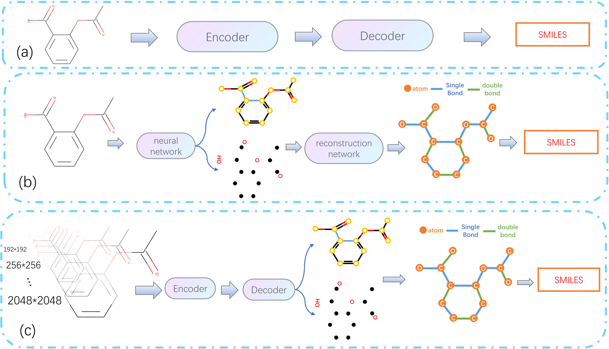 | ||
| Fig. 1 Architecture diagram of OCSR based on deep learning. (a) Simple end-to-end architecture. (b) Image–Graph–Smiles architecture. (c) Architecture of MMSSC-Net. | ||
In this paper, we propose a bottom-up cognitive processing method based on cognitive thinking. The Encoder–Decoder architecture is used to enable the neural network to perceive the atomic pixels and bond pixels of molecular vector graphics of different pixel sizes and to encode them as hidden information in the latent space using SwinV2,5 and decode it into a target sequence of molecular spatial structure using the GPT-2 Decoder method.6,7 At this point, the cognition of atoms and bonds has been transformed into the cognition of molecular structure sequences. Assemble the predicted atoms and bonds according to the molecular graph format, according to these molecular graphs, with the help of regularized expansion. They can be represented in any machine-readable format, as shown in Fig. 1(c). The main contributions of this paper are as follows:
We propose a relatively new OCSR method. Solve the problem of unstable scale of molecular vector graphics, and improves the accuracy and flexibility of OCSR.
In the recognition GPT-2 of different compound molecular sequences. It improves the accuracy of annotating molecular vector diagrams in cognitive literature.
We have innovatively expanded the end-to-end approach in OCSR, optimizing its shortcomings in looking at problems in an isolated and integrated manner. This improves the level of detail and scalability of different molecular structures in the recognition.
2 Related work
To automatically mine the correct molecular structure information from vector diagrams, a challenging task, researchers have developed various Optical Chemical Structure Recognition (OCSR) tools. Up to now, researchers have innovated based on three approaches: rule-based, machine learning, and deep learning.4 As shown in Fig. 2.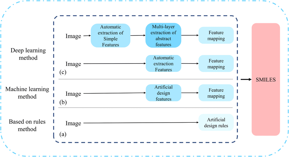 | ||
| Fig. 2 Different model methods of OCSR. (a) Is a rule-based method; (b) is a machine learning-based method; (c) is a deep learning-based method. | ||
2.1 Rule-based method
Initially, the development of OCSR systems was based on manually designed rules. In 1992, the first complete OCSR tool, Kekulé,8 was released. Kekulé generates connection tables using a rule-based approach and has a graphical user interface that supports inspection and editing of results. Subsequently, OROCS,9 CLiDE,10 CLIDE Pro,11 MolRec,12 Imago13,14 many methods have evolved and developed using a rule-based method. CLIDE Pro obtains information based on the pixels of the image and decomposes the chemical structure into graphics, wedge bonds, and characters. In text grouping, words, sentences, and small paragraphs are formed based on the collinearity of individual characters, enhancing its interpretability.11 For the parsing of atomic and superatomic labels, OSRA applies an empirically determined confidence estimation function, retaining only the best confidence value of the results,12 this allows both polymer structures and reactions to be recognized.2.2 Machine learning-based method
With the popularity of machine learning methods, the mid-term development of OCSR has followed the path of machine learning. Compared to the rule-based method of rigidly “thresholding”, artificial design features, machine learning methods that use some models for classification appear to be more flexible and accurate. Thus, a machine learning-based OCSR method was proposed. chemOCR15 is an earlier machine learning-based OCSR method, after receiving the image input, the method performs preprocessing. Use the support vector machine model (SVM) for classification and recognition of lines and nodes. Chemical machine vision16 uses Kohonen17 networks at the back end to distinguish between chemical structure images and non-chemical images. MLOCSR,18 OCSR,19 Chemrobot20 each method has its own characteristics. MLOCSR uses Markov logic networks to assign probabilities to element mappings of molecular representations, at the same time, it is stored as a knowledge base to optimize the noise problem of the information extracted by the underlying modules.42.3 Deep learning-based method
Recently, OCSR has also followed the trend of the times and entered the field of deep learning. The thinking is to use various models to extract the information features of the image, and then map them to the desired classification using feature mapping. Compared to rule-based methods, it has a larger sample size and is more universal. It is also more flexible in later maintenance and optimization. As a result, many deep learning-based methods have emerged, SwinOCSR,3 DECIMER 1.0 (ref. 4), Chemgrapher,21 EEAIC,22 ABC-Net,23 Image2SMILES24 all of these have their merits. There are mainly two forms: the end-to-end image captioning Encoder–Decoder method and the object recognition Image–Graph–Smiles method using deep neural networks. Please refer to Fig. 1. Deep learning methods have higher recognition accuracy than rigid rule-based methods, and are also convenient for later optimization. The larger the number of training samples, the better the recognition effect. But there are also certain disadvantages. For example, when the molecular graph contains different pixel sizes or large molecular representations, these methods are difficult to achieve higher accuracy.To address the current shortcomings, we have proposed a multi-stage cognitive recognition model.
3 Results and discussion
3.1 Problem design
We start with our problem statement. X ∈ Rw×h×3 and I ∈ Rp×p×3 are the molecular image space and the molecular feature mapping space. The molecular graph is transformed from the image space to the mapping feature space, and the hidden features xi are obtained by modeling between image Tokens. Therefore, We abstract MMSSC as a function, f: (Ixi,T) ↦![[T with combining tilde]](https://www.rsc.org/images/entities/i_char_0054_0303.gif) ↦ G(v,e), Ixi∈ Rp×p×3 is a set of xi, T ∈ R5×(m+n) is the true Smiles combination sequence, ∈ R5×(m+n) is the predicted Smiles combination sequence, G is the predicted molecular graph information, where n is the number of atoms and m is the number of chemical bonds. Specifically, given a combination of the molecular image hidden features and sequence {xi,ti}Ni=1, T is a set of ti (ti = {ti1,…,tik,tik+1,…,til}, {ti1,…,tik} is the true sequence of the molecule, {tik+1,…,til} is the randomly added noise sequence). Our goal is to learn how to cognitively represent different molecular images as corresponding molecular graphs G(v,e). (v = {a1,…,an} representing the set of atoms, e = {b1,…,bm} representing the set of bonds . Then, G(v,e) is regularized and expanded to generate meaningful machine-readable strings (such as Smiles).
↦ G(v,e), Ixi∈ Rp×p×3 is a set of xi, T ∈ R5×(m+n) is the true Smiles combination sequence, ∈ R5×(m+n) is the predicted Smiles combination sequence, G is the predicted molecular graph information, where n is the number of atoms and m is the number of chemical bonds. Specifically, given a combination of the molecular image hidden features and sequence {xi,ti}Ni=1, T is a set of ti (ti = {ti1,…,tik,tik+1,…,til}, {ti1,…,tik} is the true sequence of the molecule, {tik+1,…,til} is the randomly added noise sequence). Our goal is to learn how to cognitively represent different molecular images as corresponding molecular graphs G(v,e). (v = {a1,…,an} representing the set of atoms, e = {b1,…,bm} representing the set of bonds . Then, G(v,e) is regularized and expanded to generate meaningful machine-readable strings (such as Smiles).
It's just that the first output element here is not the Smiles of the previous method, but the recognition atomic target and bond target, we give a generation probability:
 | (1) |
The model adopts the cross-entropy loss with maximum likelihood estimation, which can be expressed in this article as:
 | (2) |
3.2 Model architecture
MMSSC-Net uses the Encoder–Decoder method as the basic architecture of our cognitive recognition, as shown in Fig. 3(a). We use a trained SwinV2 as the encoder for our molecular images. Specifically, the encoder maps the image to a high-dimensional latent space to generate feature maps. This gives it the ability to model within and between tokens, and applies dimensionality transformation to generate feature vectors encoded as hidden representations xi. For the generation of molecular graph G(v,e), we refer to PIX2SEQ6 and optimize it by using GPT2 and MLP to build a recognition decoder, GPT2 is used to recognize atom types, and MLP is used to recognize bond types. The encoder uses an autoregressive language model to predict the next token without considering future tokens, with the previous tokens and the encoded image representation as conditions, an atom token information is generated at a time, then by recognizing the bond information from the atom token information, the generation of the molecular graph G(v,e) can be completed. Finally, the conversion from G to Smiles is achieved by adding regularization.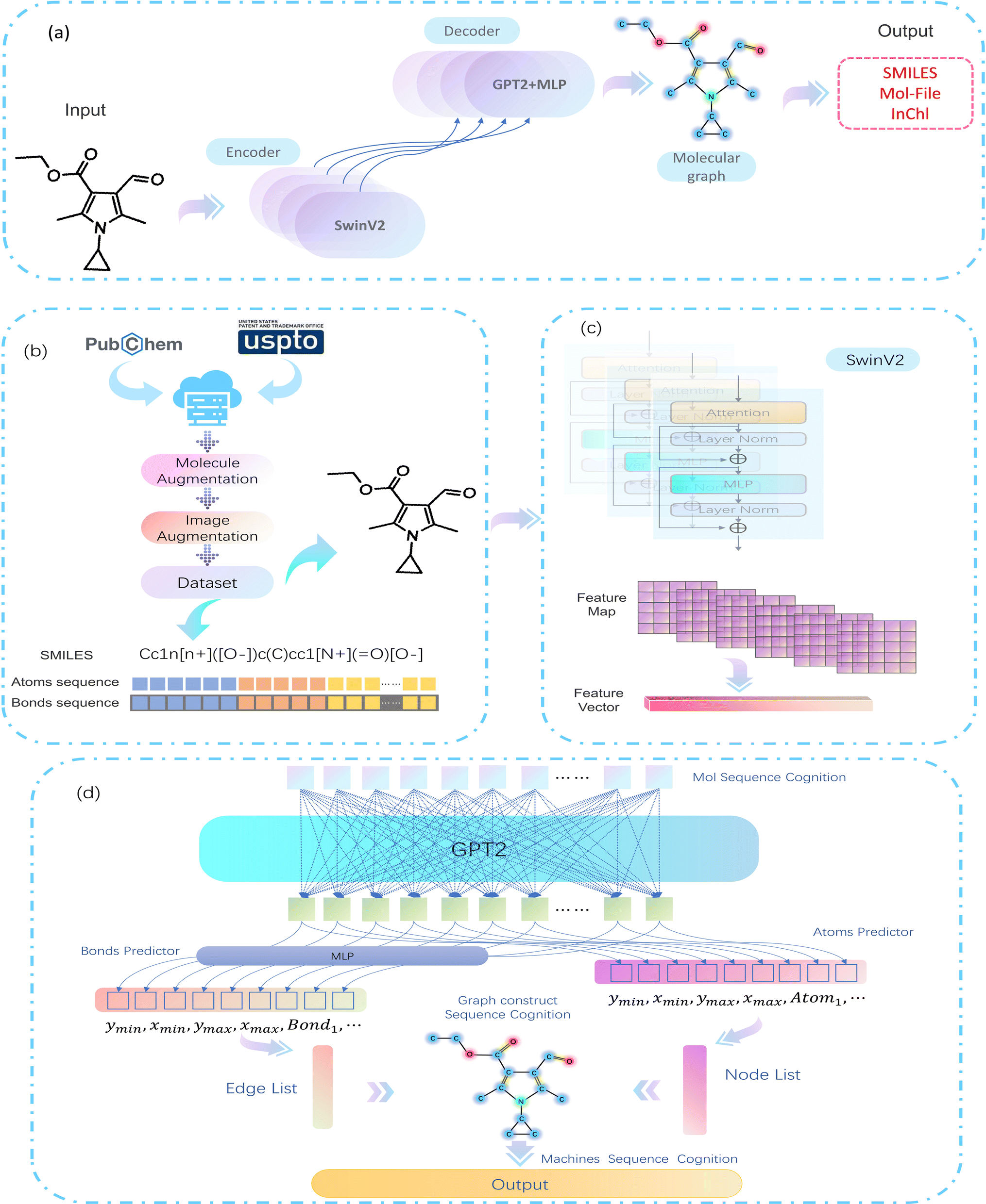 | ||
| Fig. 3 MMSSC-Net model flowchart. (a) Overview of the MMSSC model. (b) Experimental data preprocessing. (c) Molecular image feature representation module. (d) Target sequence prediction. | ||
3.3 Atomic sequence recognition
Let the input be a molecular image X ∈ Rw×h×3, cut into B disjoint patch regions, and mark some regions as I ∈ Rp×p×3, where {W,H} and {P,P} represent the size of the input image and the patch region, respectively, and N = (H × W)/P2 is the data of the patch region, that is, the effective sequence length of the input to the encoder. The effective sequence patch vector is input to SwinV2 for four encoding stages for hierarchical visual representation. The feature output from the last stage of SwinV2 is used as the molecular image feature xi. The process can be represented as follows:| xi = {xi1,xi2,…,xiM} = F(SwinV2(X)) | (3) |
![[T with combining macron]](https://www.rsc.org/images/entities/i_char_0054_0304.gif) 1:j−1 = {ymin, xmin, ymax, xmax, Cn,⋯} 1:j−1 = {ymin, xmin, ymax, xmax, Cn,⋯}
| (4) |
![[t with combining macron]](https://www.rsc.org/images/entities/i_char_0074_0304.gif) i1 = {ymin, xmin, ymax, xmax, C1} i1 = {ymin, xmin, ymax, xmax, C1}
| (5) |
In order to make the model have generalization ability for different molecular target images and cognitive ability for different forms of atoms, a random sequence Tr is added as a suffix in the target and input sequences. In the standard training process, this suffix will be automatically optimized to guide the GPT2 model toward new goals.25
Suffix random sequence:
| Tr = {ymin, xmin, ymax, xmax, Crand,⋯} | (6) |
|
tij = ij ⊗ Tr
| (7) |
|
T1:j−1 = 1:j−1 ⊗ Tr
| (8) |
![[t with combining tilde]](https://www.rsc.org/images/entities/i_char_0074_0303.gif) ij = {ỹmin, ij = {ỹmin, ![[x with combining tilde]](https://www.rsc.org/images/entities/i_char_0078_0303.gif) min, ỹmax, max, min, ỹmax, max, ![[C with combining tilde]](https://www.rsc.org/images/entities/i_char_0043_0303.gif) n,⋯} n,⋯}
| (9) |
Thus, we can obtain the autoregressive generation of atomic prediction, that is:
 | (10) |
| v = {ymin, xmin, ymax, xmax, C1, …, ymin, xmin, ymax, xmax, Cn} | (11) |
The goal of the atomic predictor shown in Fig. 3(d) is to transform atomic information in the image space into atomic sequence space information, and the prediction of sequence-driven sequence can realize atomic cognition in this model. Under the guidance of the language model GPT2 output, predict the next atom one by one.
3.4 Chemical bond sequence recognition
The chemical bond is the general term for the strong interaction force between two or more adjacent atoms (or ions) within a pure substance molecule or crystal. Therefore, our prediction of bonds is based on the spatial position of atoms, connecting the spatial position coordinates of atoms as the bond information b between atoms, using it as the target sequence, and predicting the bond in the same way as the atomic prediction. And used the connected atoms to construct bond information for prediction. The specific prediction is:| bα,β = Cα‖Cβ | (12) |
Bond sequence set:
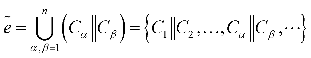 | (13) |
 | (14) |
| e = {b1, …, bm} = MLP(ẽ) | (15) |
As shown in Fig. 3(d), the set of atoms recognized by cognition v = {a1,…,an} is transformed into the node set V of the molecular graph, the set of chemical bonds e = {b1,…,bm} is transformed into the edge set E of the molecular graph, the molecular graph structure can be constructed from nodes and edges, and then the molecular graph structure is represented in the required machine-readable format (such as Smiles, etc).
3.5 Decoding vocab
In order to make the decoder easier to understand and recognize SMILES characters, we have constructed two dictionaries of character types, one for atom and bond information, and one for bond and isomer information. In the bond and atom dictionary, in addition to having the sequence start and end symbols [sos] and [eos], we have added 95 common numbers and characters to the dictionary, For example: [0], [1], [2], [3], [4], [5], [6], [7], [8], [9], [C], [l], [C], [O], [N], [N], [F], [H], [O], [S], [B], [r], [I], [P], [=], etc. In the key and isomer information dictionary, we have added 2000 characters to the dictionary based on the SMARTS rules, such as: “[Qs]”, “[X14]”, “[C2F5]”, “[CH)m]”, “[(R4)a]”, “[halo]”, “[OR20]”, “[(R13)b]”, “[X5]”, etc., referring to USPTO and ChEMBL. Thus, our cognitive model can also learn the corresponding SMILES and SMARTS paradigms.4 Experiment
4.1 Dataset
Our data mainly comes from the PubChem database and the United States Patent and Trademark Office (USPTO).PubChem database:26 We collected 1 million molecules, mainly containing two-dimensional image structures and molecular labels. The molecules obtained from PubChem were originally in InChI format, and then converted to SMILES format using Indigo, in order to ensure that the model does not overly strengthen the features of a certain type of molecular image, we completely base the sampling of molecules on randomness.
USPTO:27 We collected 600![[thin space (1/6-em)]](https://www.rsc.org/images/entities/char_2009.gif) 000 data from the patent grants issued by the United States Patent and Trademark Office (USPTO), including molecular images and structural labels. USPTO data provides molecules in MOL format, which are then converted to SMILES format using Indigo.
000 data from the patent grants issued by the United States Patent and Trademark Office (USPTO), including molecular images and structural labels. USPTO data provides molecules in MOL format, which are then converted to SMILES format using Indigo.
4.2 Data augmentation
4.3 Experimental setup
For the molecular image encoder, we use the pre-trained Swin Transformer V2 model on ImageNet-1K, where the window size is 16 × 16, containing 88M parameters, and the resolution of the image input is 256 × 256. By adopting scaled cosine attention to improve attention control between molecular pixels. And applying the log-space continuous position bias method to fine-tune tasks with arbitrarily changing window sizes, it is convenient for cognition between different pixels. For the decoder, we use a 24-layer GPT-2 with 12 attention heads, a hidden dimension of 768, and a dropout probability of 0.1. The processing batch size of MMSSC-Net is 128, the learning rate is 4 × 10⁻⁵, and it is trained for 40 epochs at the same time. According to the purpose of the experiment for different factors, the variable control method is used to conduct different factor experiments. The enhanced dataset of PubChem and USPTO is divided into training and test sets at a ratio of 8:2. For the evaluation of the model. We use five public databases: STAKER, USPTO, CLEF, JPO, and UOB. As shown in Table 1.
| Evaluate dateset | Num | Average resolution |
|---|---|---|
| STAKER | 40000 |
256 × 256 |
| USPTO | 4862 | 721 × 432 |
| CLEF | 881 | 1245 × 412 |
| JPO | 380 | 614 × 367 |
| UOB | 5720 | 759 × 416 |
Accuracy shows the exact string match between the input known as Smile and the Smile of this model. At the same time, under this metric, the result is only correct when the generated SMILES sequence is the same as the original sequence. This metric analyzes the recognition accuracy at the entire molecular level.
The similarity between the generated molecular fingerprint spectrum and the original molecular fingerprint spectrum is measured using the Tanimoto coefficient. This metric analyzes the molecular similarity level and lays the foundation for downstream tasks such as molecular property prediction. At the same time, the Morgan fingerprint is used to represent molecules, and then the molecular similarity is calculated based on the Tanimoto coefficient.
4.4 Comparison with other tools
We compare the model with other existing methods. To distinguish between different models, we have divided them into three categories: the first category is rule-based MolVec30 and OSRA.34 The second category is the Image–Smiles method with molecular image information as the main information, such as ABC-Net,23 Img2Mol,35 and MolMiner.31 The third category is the Image–Graph–Smiles method that converts molecular images into molecular graphs with structural information as the main information, such as Image-To-Graph,32 MolScribe,33 and ChemGrapher.36Table 2 and Fig. 3 shows the recognition accuracy of different models. MMSSC-Net achieved higher scores than existing systems in most benchmark tests, and the ACC values in the first three datasets are above 94%. Among the two rule-based methods, MolVec and OSRA only showed good results in the first two synthetic datasets, but the ACC in the real datasets was not satisfactory, and the performance of the rule-based methods on the staker dataset dropped significantly in terms of ACC. This is because the rule-based method does not have corresponding rules for noise processing when dealing with noisy datasets. At the same time, it can also be seen from Table 2 that the performance of rule-based tools on high-resolution datasets is lower than that on low-resolution datasets. This indicates that they are more sensitive to changes in molecular image resolution than to changes in noise. In the five real datasets, although MolVec and OSRA are both sensitive to changes in noise and resolution, overall observation shows that the change in accuracy of OSRA is less than that of MolVec, indicating that OSRA is more robust.
| Model | Indigo | RDKit | USPTO | CLEF | UOB | Staker | JPO | |
|---|---|---|---|---|---|---|---|---|
| MolVeco,30 | Accuracy | 95.63 | 86.7 | 88.47 | 81.61 | 81.32 | 4.49 | 66.8 |
| Tanimoto | 98.88 | 96.54 | 95.98 | 92.65 | 93.15 | 20.21 | 88.63 | |
| OSRA12 | Accuracy | 95.4 | 87.3 | 87.4 | 84.6 | 78.5 | 0.6 | 55.3 |
| Tanimoto | 98.69 | 95.3 | 94.85 | 92.63 | 89.27 | 5.64 | 75.35 | |
| ABC – Neto,23 | Accuracy | 96.4 | 98.3 | * | * | 96.1 | * | * |
| Tanimoto | 98.9 | 99.6 | * | * | 98.9 | * | * | |
| Img2Molo,22 | Accuracy | 79 | 93.4 | 42.29 | 48.84 | 78.18 | 64.33 | 45.14 |
| Tanimoto | 91.5 | 97.4 | 73.07 | 78.04 | 88.51 | 83.76 | 69.43 | |
| MolMinero,31 | Accuracy | * | * | 89.9 | 84.6 | 90 | * | 72.2 |
| Tanimoto | * | * | * | * | * | * | * | |
| Image – To – Grapho,32 | Accuracy | * | * | 55.1 | 51.7 | 82.9 | * | 50.3 |
| Tanimoto | * | * | * | * | * | * | * | |
| MolScribeo,33 | Accuracy | 97.5 | 93.8 | 92.6 | 86.9 | 87.9 | 86.9 | 76.2 |
| Tanimoto | 99 | 97.5 | 97.5 | 90.5 | 96 | 97.8 | 88.1 | |
| ChemGraphero,21 | Accuracy | * | * | 70.6 | * | * | * | * |
| Tanimoto | * | * | * | * | * | * | * | |
| MMSSC-Net | Accuracy | 98.14 | 94.91 | 94.24 | 91.26 | 92.71 | 89.44 | 75.48 |
| Tanimoto | 99.56 | 98.82 | 98.81 | 96.78 | 97.24 | 95.45 | 89.32 | |
In the Image–Smiles method, some show a high level, especially ABC-Net, which is above 96% in both RDKit and UOB data. This is directly related to its use of heat map technology to predict atom, bond, and charge classification, but its performance for different resolutions is not relevant, indicating that there are some flaws. Img2Mol has made a contribution in the resolution-sensitive test. The perception of real data is not so sensitive, resulting in an overall accuracy of less than 80%. At the same time, although Image–Smiles has good results in Indigo and RDKit recognition, this method lacks interpretability of molecular images and does not clearly introduce chemical structure and rules.
The last method, Image–Graph–Smiles, is currently a more refined work. Although Image-To-Graph is also based on this method, there are deficiencies in the recognition of atoms and bonds to the assembly of molecular graphs, resulting in its performance not being so ideal. Our method takes into account changes in resolution and molecular graph structure information in a more refined way. It has achieved good results in real data at different resolutions, but there is still room for improvement in some real data such as JPO.
4.5 Ablation study
To demonstrate that the MMSSC-Net is more cognitively capable of changes in resolution, Table 3 shows the different effects of changing our visual encoder. We evaluated the performance of Swin transformer,37 Vit-B,38 and ResNet-50 as backbone encoders. From Table 3, it can be seen that MMSSC-Net has shown great performance on most real datasets. This is because the model we use is more flexible in expanding the window resolution, making the model more adaptable to molecular images at different resolutions. And during the experiment, the time taken by Swin transformer and Vit-B was much higher than MMSSC-Net, showing that the efficiency of MMSSC-Net is greater than the other three. For ResNet-50, because our overall model is cognitive between sequences, NLP-based visual encoders (Swin transformer and Vit-B) are better able to perform their due performance in this task. Therefore, the recognition accuracy of ResNet-50 in this task is not satisfactory. From this experiment, we can conclude that MMSSC-Net has good cognitive recognition performance in terms of molecular recognition efficiency and different molecular image resolutions.| Encoder | USPTO | CLEF | UOB | Staker | JPO |
|---|---|---|---|---|---|
| SwinTransformer | 90.26 | 85.41 | 88.57 | 87.85 | 79.15 |
| Vit-B | 86.58 | 72.27 | 79.69 | 75.31 | 71.9 |
| ResNet-50 | 78.06 | 67.21 | 72.52 | 71.51 | 65.62 |
| MMSSC-Net | 94.24 | 91.26 | 92.71 | 89.44 | 75.48 |
4.6 Case study
From the result comparison experiment, we can see that for the OCSR task, the change of the dataset is also very sensitive. In order to better study the predictive performance and future development of the MMSSC-Net, we randomly selected samples from four datasets for analysis. Fig. 4(a) shows representative examples from these four datasets. In noisy datasets, some noise points may cause the model to misidentify (Fig. 5). The last dataset comes from DECIMER,39 it can better reflect the robustness of MMSSC-Net. When dealing with irrelevant text and symbols in the dataset, such as irrelevant information in JPO and DECIMER, it is difficult for the model to recognize because this is unexpected noise that has not been observed in MMSSC-Net. | ||
| Fig. 4 Resolution analysis. (a) Represents the analysis of different image resolutions using deep learning methods. (b) Represents the analysis of different image resolutions using rule-based methods. | ||
 | ||
| Fig. 5 Case analysis. (a) Selected data. (b) CLEF case. (c) JPO case. (d) STAKER case. (e) DECIMER case. | ||
Furthermore, Fig. 4(a) is an analysis of incomplete predictions. Overall, MMSSC-Net is able to recognize most molecular images. Especially for sample images and high-resolution images that have not participated in learning during training, it has good performance, but the presence of stereochemical bonds in the dataset often leads to the existence of errors. This may be due to the spatial information error when representing three-dimensional information with two-dimensional information. In Fig. 4(b) and (c), there are errors in recognizing virtual wedge bonds as solid wedge bonds and single bonds as solid wedge bonds. In addition to spatial errors, the gap in the representation of stereochemical bonds in molecular graphs when MMSSC-Net converts molecular images into molecular graphs and then into Smiles is also the cause of its errors. In Fig. 4(d), most of the errors are caused by the incomplete recognition of virtual wedge bonds and solid wedge bonds. The reason is that the molecular image is encoded in three-channel chroma. Hand-drawn molecules often cannot completely fill the space required for virtual wedge bonds and solid wedge bonds with one color, which leads to the introduction of blank color systems during recognition and the occurrence of errors.
5 Conclusions
In this paper, we propose a deep learning-based cognitive approach, MMSSC-Net, for molecular sequence recognition. MMSSC-Net is based on the encoder–decoder image captioning method and is built on top of it, allowing the model to cognitively construct molecular graphs by recognizing atomic sequences and bond sequences from molecular images, and then converting them into machine-readable sequences. Under this approach, we validated the effectiveness of MMSSC-Net on five real datasets, and discussed the impact of data changes and model changes on the structure of MMSSC-Net through the different characteristics of the datasets. In MMSSC-Net, which can jointly learn high-dimensional representations and may improve downstream tasks involving high-resolution molecular images. In addition, we also conducted a visual case study of the conversion from molecular images to molecular graphs and the conversion of real samples to Smiles, providing intuitive insights for future research.Data availability
The source code of the proposed method is openly available at: https://github.com/Wzew5Lp/MMSSCNet.Author contributions
D. H. Z. and J. L. conceptualized the project. D. Z. and Z. W. W. performed the experimental studies. D. Z. and Z. W. W. prepared the manuscript.Conflicts of interest
There are no conflicts to declare.Acknowledgements
The authors acknowledge the financial support from the foundation: Natural Science Foundation of China (62362066,62366059), and Natural Science Foundation of Yunnan Province (202001BB050052).Notes and references
- S. Ekins, A. C. Puhl, K. M. Zorn, T. R. Lane, D. P. Russo, J. J. Klein, A. J. Hickey and A. M. Clark, Nat. Mater., 2019, 18, 435–441 CrossRef CAS PubMed.
- J. Vamathevan, D. Clark, P. Czodrowski, I. Dunham, E. Ferran, G. Lee, B. Li, A. Madabhushi, P. Shah and M. Spitzer, et al., Nat. Rev. Drug Discovery, 2019, 18, 463–477 CrossRef CAS PubMed.
- Z. Xu, J. Li, Z. Yang, S. Li and H. Li, J. Cheminf., 2022, 14, 1–13 Search PubMed.
- K. Rajan, H. O. Brinkhaus, A. Zielesny and C. Steinbeck, J. Cheminf., 2020, 12, 1–13 Search PubMed.
- Z. Liu, H. Hu, Y. Lin, Z. Yao, Z. Xie, Y. Wei, J. Ning, Y. Cao, Z. Zhang, L. Dong, et al., Swin transformer v2: Scaling up capacity and resolution, Proceedings of the IEEE/CVF conference on computer vision and pattern recognition, 2022, pp. 12009–12019 Search PubMed.
- T. Chen, S. Saxena, L. Li, D. J. Fleet and G. Hinton, Pix2seq: A language modeling framework for object detection, arXiv, 2021, preprint, arXiv:2109.10852, DOI:10.48550/arXiv.2109.10852.
- A. Radford, J. Wu, R. Child, D. Luan, D. Amodei, I. Sutskever, et al., OpenAI blog, 2019, vol. 1, p. 9 Search PubMed.
- J. R. McDaniel and J. R. Balmuth, J. Chem. Inf. Comput. Sci., 1992, 32, 373–378 CrossRef CAS.
- R. Casey, S. Boyer, P. Healey, A. Miller, B. Oudot and K. Zilles, Optical recognition of chemical graphics, Proceedings of 2nd International Conference on Document Analysis and Recognition (ICDAR’93), IEEE, 1993, pp. 627–631 Search PubMed.
- P. Ibison, M. Jacquot, F. Kam, A. Neville, R. W. Simpson, C. Tonnelier, T. Venczel and A. P. Johnson, J. Chem. Inf. Comput. Sci., 1993, 33, 338–344 CrossRef CAS.
- A. T. Valko and A. P. Johnson, J. Chem. Inf. Model., 2009, 49, 780–787 CrossRef CAS PubMed.
- N. M. Sadawi, A. P. Sexton and V. Sorge, CLEF (Online Working Notes/Labs/Workshop), 2012, pp. 17–20 Search PubMed.
- I. V. Filippov and M. C. Nicklaus, J. Chem. Inf. Model., 2009, 49, 740–743 CrossRef CAS PubMed.
- V. Smolov, F. Zentsev and M. Rybalkin, Imago: Open-Source Toolkit for 2D Chemical Structure Image Recognition, Text Retrieval Conference, 2011 Search PubMed.
- M. Zimmermann, TREC, 2011 Search PubMed.
- G. V. Gkoutos, H. Rzepa, R. M. Clark, O. Adjei and H. Johal, J. Chem. Inf. Comput. Sci., 2003, 43, 1342–1355 CrossRef CAS PubMed.
- T. Kohonen and T. Honkela, Scholarpedia, 2007, 2, 1568 CrossRef.
- P. Frasconi, F. Gabbrielli, M. Lippi and S. Marinai, J. Chem. Inf. Model., 2014, 54, 2380–2390 CrossRef CAS PubMed.
- C. Hong, X. Du and L. Zhang, 2015 Joint International Mechanical, Electronic and Information Technology Conference (JIMET-15), 2015, pp. 267–271 Search PubMed.
- S. D. Pineda Flores, J. Chem. Theory Comput., 2021, 17, 4028–4038 CrossRef CAS PubMed.
- M. Oldenhof, A. Arany, Y. Moreau and J. Simm, J. Chem. Inf. Model., 2020, 60, 4506–4517 CrossRef CAS PubMed.
- C. Sundaramoorthy, L. Z. Kelvin, M. Sarin and S. Gupta, arXiv, 2021, preprint, arXiv:2104.14721, DOI:10.48550/arXiv.2104.14721.
- X.-C. Zhang, J.-C. Yi, G.-P. Yang, C.-K. Wu, T.-J. Hou and D.-S. Cao, Briefings Bioinf., 2022, 23, bbac033 CrossRef PubMed.
- I. Khokhlov, L. Krasnov, M. V. Fedorov and S. Sosnin, Chemistry-Methods, 2022, 2, e202100069 CrossRef CAS.
- C.-Y. Lin and F. J. Och, Proceedings of the 42nd Annual Meeting of the Association for Computational Linguistics (ACL-04), 2004, pp. 605–612 Search PubMed.
- S. Kim, J. Chen, T. Cheng, A. Gindulyte, J. He, S. He, Q. Li, B. A. Shoemaker, P. A. Thiessen and B. Yu, et al., Nucleic Acids Res., 2019, 47, D1102–D1109 CrossRef PubMed.
- D. Pavlov, M. Rybalkin, B. Karulin, M. Kozhevnikov, A. Savelyev and A. Churinov, J. Cheminf., 2011, 3, P4 Search PubMed.
- S. J. Graham, G. Hancock, A. C. Marco and A. F. Myers, J. Econ. Manag. Strategy, 2013, 22, 669–705 CrossRef.
- D. Pavlov, M. Rybalkin and B. Karulin, et al., J. Cheminf., 2011, 3(suppl 1), P4 Search PubMed.
- T. Peryea, D. Katzel, T. Zhao, N. Southall and D.-T. Nguyen, Abstr. Pap. Am. Chem. Soc., 2019, 258 Search PubMed.
- Y. Xu, J. Xiao, C.-H. Chou, J. Zhang, J. Zhu, Q. Hu, H. Li, N. Han, B. Liu and S. Zhang, et al., J. Chem. Inf. Model., 2022, 62, 5321–5328 CrossRef CAS PubMed.
- S. Yoo, O. Kwon and H. Lee, ICASSP 2022-2022 IEEE International Conference on Acoustics, Speech and Signal Processing (ICASSP), 2022, pp. 3393–3397 Search PubMed.
- Y. Qian, J. Guo, Z. Tu, Z. Li, C. W. Coley and R. Barzilay, J. Chem. Inf. Model., 2023, 63, 1925–1934 CrossRef CAS PubMed.
- I. V. Filippov and M. C. Nicklaus, J. Chem. Inf. Model., 2009, 49, 740–743 CrossRef CAS PubMed.
- D.-A. Clevert, T. Le, R. Winter and F. Montanari, Chem. Sci., 2021, 12, 14174–14181 RSC.
- M. Oldenhof, A. Arany, Y. Moreau and J. Simm, J. Chem. Inf. Model., 2020, 60, 4506–4517 CrossRef CAS PubMed.
- Z. Liu, Y. Lin, Y. Cao, H. Hu, Y. Wei, Z. Zhang, S. Lin and B. Guo, Proceedings of the IEEE/CVF international conference on computer vision, 2021, pp. 10012–10022 Search PubMed.
- K. Han, Y. Wang, H. Chen, X. Chen, J. Guo, Z. Liu, Y. Tang, A. Xiao, C. Xu and Y. Xu, et al., IEEE Trans. Pattern Anal. Mach. Intell., 2022, 45, 87–110 Search PubMed.
- H. O. Brinkhaus, A. Zielesny, C. Steinbeck and K. Rajan, J. Cheminf., 2022, 14, 1–4 Search PubMed.
| This journal is © The Royal Society of Chemistry 2024 |