 Open Access Article
IUPAC recommended experimental methods and data evaluation procedures for the determination of radical copolymerization reactivity ratios from composition data†
Anton A. A.
Autzen
a,
Sabine
Beuermann
 b,
Marco
Drache
 b,
Christopher M.
Fellows
c,
Simon
Harrisson
 d,
Alex M.
van Herk
 *ef,
Robin A.
Hutchinson
 g,
Atsushi
Kajiwara
 h,
Daniel J.
Keddie
 i,
Bert
Klumperman
 j and
Gregory T.
Russell
 k
k
aDepartment of Health Technology, Technical University Denmark, Denmark
bInstitute of Technical Chemistry, Clausthal University of Technology, Germany
cSchool of Science and Technology, University of New England, Australia
dLCPO, UMR 5629, CNRS/Bordeaux-INP/University of Bordeaux, Pessac, France
eDepartment of the Built Environment, Eindhoven University of Technology, The Netherlands. E-mail: a.m.v.herk@tue.nl
fSchool of Materials Science and Engineering, Nanyang Technological University, Singapore
gDepartment of Chemical Engineering, Queens University, Canada
hDepartment of Materials Science, Nara University of Education, Japan
iSchool of Chemistry, University of Nottingham, England, UK
jDepartment of Chemistry and Polymer Science, University of Stellenbosch, South Africa
kSchool of Physical and Chemical Sciences, University of Canterbury, Christchurch, New Zealand
First published on 11th April 2024
Abstract
The IUPAC working group on “Experimental Methods and Data Evaluation Procedures for the Determination of Radical Copolymerization Reactivity Ratios” recommends a robust method to determine reactivity ratios from copolymer composition data using the terminal model for copolymerization. The method is based on measuring conversion (X) and copolymer composition (F) of three or more copolymerization reactions at different initial monomer compositions (f0). Both low and high conversion experiments can be combined, or alternatively only low conversion experiments can be used. The method provides parameter estimates, but can also reveal deviations from the terminal model and the presence of systematic errors in the measurements. Special attention is given to error estimation in F and construction of the joint confidence interval for reactivity ratios. Previous experiments measuring f0 − F or f − X can also be analyzed with the IUPAC recommended method. The influence of systematic errors in the measurements on the reactivity ratio determinations is investigated, including ways to identify and mitigate such errors.
Introduction of the method
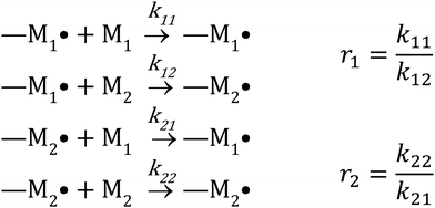
There are several kinetic models describing the incorporation of monomers into polymer chains during radical copolymerizations,1 of which the terminal model, where only the last unit in the chain affects the reactivity of a chain-end radical, is the most widely applied for copolymer composition. Other models include the penultimate model,2 in which the penultimate unit also affects the reactivities, and the non-terminal model, where the chain ends do not affect reactivities. The non-terminal model only applies to the special case of ideal copolymerization, where there is no difference in reactivity for the monomers towards the propagating species.3 Then there are several models to cater for complexation between monomers (the complex participation model) or complexation between monomer and polymer chain end (the bootstrap model).4 Copolymerization models serve to create mechanistic understanding of copolymerization reactions, but are ultimately most important in modelling of composition in manufacturing of copolymers. A high conversion is typically pursued for commercial manufacturing of copolymers. For batch reactions, or reactions conducted in a plug-flow reactor, high conversion almost inevitably leads to composition drift, i.e. the shift in monomer and copolymer composition due to different monomer consumption rates. In conventional radical copolymerizations, composition drift results in heterogeneous copolymers. In reversible-deactivation radical polymerizations, however, drift in monomer composition results in a gradient in the composition of all the growing polymer chains, which can be a desirable feature for generating gradient copolymers.5The core assumption of the terminal copolymerization model is that the reactivity of the growing chains is entirely determined by their final monomer unit. Thus a copolymerization of two monomers, M1 and M2, contains two types of growing chains, and a total of four propagation reactions, as shown in Scheme 1.6 Reactivity ratios,1ri are defined as the ratio of the rate coefficients of propagation kii and kij, corresponding to homopropagation and crosspropagation of chains containing a terminal unit Mi.
Defining fi as the mole fraction of Mi in the comonomer mixture (fi = [Mi]/([M1] + [M2])), and and Fiinst as the mole fraction of Mi that is instantaneously being incorporated into the copolymer (Fiinst = d[Mi]/d([M1] + [M2]), gives the well-known Mayo–Lewis7 copolymer composition equation (eqn (1)):
 | (1) |
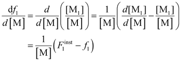
Differentiating f1 with respect to the total monomer concentration (eqn (2)) and integration after separation of variables leads to the Skeist equation8 (eqn (3)) relating total monomer conversion, X, to the change in monomer composition:
 | (2) |
 | (3) |
The Skeist equation may be solved numerically. Alternatively, an analytical solution to this equation was provided by Meyer and Lowry9 (eqn (4)) which relates X to the current monomer composition fi and the initial monomer composition fi0.
 | (4) |
It should be noted that this equation contains singularities at r1 = 1, r2 = 1 and r1 + r2 = 2 and these can complicate its utilization (for specific solutions at the singularities see ESI-1†).
Finally, the cumulative monomer composition, F1cum can be obtained from eqn (5).
 | (5) |
Reactivity ratios play a central role in eqn (1)–(4), but as the equations are non-linear in nature, it is not immediately evident how to determine these reactivity ratios from experimental data. Several methods have been proposed over the last 75 years, many of which involve linearization of the copolymer composition equation. Widely used linearized methods such as Fineman–Ross10 and Kelen–Tüdős11 distort the error structure of the experimental data, however, and can lead to biased and imprecise results. For this reason, non-linear least squares fitting (NLLS) is greatly preferred. Further problems are encountered when the assumptions of the models are violated: for example, by applying eqn (1) to copolymerizations with non-negligible conversion, where eqn (4) would be more appropriate. These incorrect procedures can lead to significant errors in the estimation of reactivity ratios.
One of the early advocates of establishing methods for determining reactivity ratios more correctly was Prof. Ken O'Driscoll. In a recent paper on his work6 we presented his insights, which we fully support and which formed the basis of this present work of our IUPAC working group on “Methods and Data Evaluation Procedures for the Determination of Radical Copolymerization Reactivity Ratios”.
From ref. 6 we repeat the eight key insights:
1. Model discrimination and parameter estimation normally require two different sets of experiments.
2. To apply the instantaneous copolymer composition equation (eqn (1)), low conversion data needs to be used (O'Driscoll indicates < 5% conversion).
3. The outcome of the statistical method applied should not depend on the indexing of the monomers (i.e., whether a monomer is designated M1 or M2) (many workers do not realise that this is commonly a problem).
4. The starting point of the calculation should not affect the estimates (this is in reference to the use of iterative methods to find the optimal values).
5. Linearized methods cannot be expected to give good estimates of the reactivity ratios due to distortion of the error structure by the linearization process.
6. Correct design of experiments is of great importance.
7. Results should be reported as a point estimate together with a joint confidence interval (JCI).
8. If there is also an error in the monomer composition (fi), the errors in (all) variables method (EVM) should be used, and this is especially relevant for the determination of reactivity ratios from conversion dependent data using the integrated copolymerization equation (eqn (4)).
O'Driscoll also pointed out that the ease of doing the calculation plays an important role in the choice of the method, writing “The ease criterion was, even in 1970, satisfied by the “advent of the digital computer” (unfortunately, the subsequent advent of the pocket calculator with its linear least squares button has made the Fineman-Ross and related techniques seem more convenient)”.12 The unavailability of a simple-to-use NLLS computer program likely contributed to the continued use of linearized methods by many researchers. In the early 1990s O'Driscoll therefore worked with Reilly and others at the University of Waterloo to develop a microcomputer program, RREVM, based on the errors in all variables method (EVM) in order to alleviate this issue.13
In 1995 van Herk attempted to simplify NLLS fitting through visualization of the sum of squares space (VSSS), a method that can be easily implemented by scientists themselves in Visual Basic, Python or any other computer language.14 The VSSS method maps the weighted sum of squares of residuals in a large parameter space (a grid of r1 and r2) and simply finds the lowest value (the minimum) to be the optimal parameter set for the reactivity ratios.14 It was also stressed that proper weighing of the data (with their individual errors) is important to obtain correct reactivity ratios and joint confidence intervals.14–16 Until recently this was the only rigorous approach to obtain unbiased estimates and unbiased errors for arbitrary non-linear models.17
However last year a new correct method was introduced using a Bayesian hierarchical approach addressing the issue of a non-Gaussian structure of the error estimates that is a consequence of the nonlinearity of the copolymerization model.17
Unfortunately, today many researchers still use linearized methods. In 2023 alone, more than 400 papers using the Finemann–Ross method10 were reported. Furthermore, several papers were published using copolymer compositions determined at too high conversions, where composition drift will be significant, and eqn (1) cannot be used. Another issue is that some works report incorrect joint confidence intervals (see ref. 18 for a re-evaluation of a collection of published data). Even worse, many works report no uncertainty or JCI at all.
In this paper we present an example of the application of NLLS using the VSSS method keeping in mind the eight core insights of O'Driscoll.
Data collection
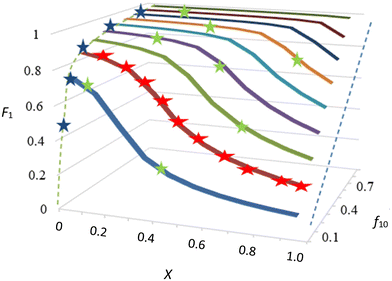
There is, however, no unique interpretation of “low conversion” in the f0 − F method, as with unfavorable reactivity ratios, strong composition drift can occur even at conversions below 5%. This may introduce significant errors in F (point 2 of O'Driscoll and see Fig. 1).
We therefore investigated several methods to correct for shifts in F at lower conversions. This includes, amongst others, using the average monomer composition over the conversion range instead of f0. However, all of these approximate correction strategies require knowledge of the conversion, suggesting that direct application of an integrated form of the copolymer equation such as the Meyer–Lowry equation (eqn (4)) is then possible. In such a case application of the integrated expression is preferable.
The way copolymerization experiments are performed does not change with this approach, but the measured conversion is now taken explicitly into account.
This also means that there is no longer any real difference between low and high conversion experiments, as in both cases copolymer composition and conversion are measured, starting from a particular f0. Low and higher conversion data may be mixed to calculate reactivity ratios. This is illustrated in Fig. 1, where data points are fitted on a f0, X, F surface. Other methods using low conversion data or measuring f − X data from a single f0 can still be seen as special cases of this more general preferred method of performing several experiments starting with different f0 values. It is also very important to have error estimates for the F value, either directly measured or calculated from changes in monomer concentrations.15,16 Note that the error in F is very different depending on whether it was measured directly or calculated from changes in f.
In this approach, both F and X may be expected to be subject to experimental errors, and as such the error in variables method (EVM) is preferred. However, in many cases it is likely that errors in determination of X will be small relative to errors in determination of F, as the measurement of X is more straightforward. In these cases, X can be treated as the error-free independent variable for the purposes of fitting.
It is also important to weight data appropriately. For example, if the experimentally obtained data is copolymer composition (F) and conversion (X), but the data is fitted using the Meyer–Lowry equation (eqn (4)), which relates the comonomer composition (f) and conversion (X), calculated f values should be weighted using Gaussian propagation of errors, as follows (note, an error in f0 is not taken into account in this equation):
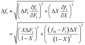 | (6) |
In the current approach we use f0 − X − F data and make the physically reasonable assumption that the major error is in F. Besides comparing the errors per datapoint, the overall error estimated by the user and the overall error obtained from the fit (sF) can also be compared using a Fisher test (see for example ESI-Tables 4 and 5†).
 | (7) |
In the case where f is monitored as a function of conversion (for example with in situ NMR20), these values can easily be converted to f0 − X − F data via the mass balance (eqn (5)). As O'Driscoll highlighted in point 8, a non-negligible error in f0 or f should be taken into account. In the conversion, the errors assumed in f and X are then converted to errors in F through Gaussian error propagation (note, an error in f0 is not included in this equation):
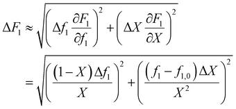 | (8) |
We believe the best option is to do the calculations with f0 − X − F data and not directly with the f0 − f − X data, because in the end we are interested in the best values for the reactivity ratios for predicting copolymer compositions. In the f0 − f − X approach a potential problem is that some of the monomer can evaporate if the reactor is not a closed system, so even if f data are converted into F data it is advised to measure at least the final average composition of the copolymer to check for internal consistency.
It is likely that the analysis of f0 − f − X data and the analysis of those data converted into f0 − X − F might give slightly different results (see ESI-Tables 7–9†) if EVM is not used. This is due to the fact that in the f0 − f − X approach fitting is of the conversion data, X, while in the f0 − X − F approach, fitting is on the composition data, F. The latter is the more robust approach and furthermore the desired application of the reactivity ratios is to predict the composition of the copolymer. Another advantage is that in the conversion from f0 − f − X to f0 − X − F both the errors in f (and if needed f0) and in X can be taken into account and through error propagation this gives a well estimated error in the calculated F (eqn (8)). This should also result in more realistic errors for the reactivity ratios. Note that this is not a full errors-in-variables method as the result is only optimized on the copolymer composition F. Proper weighting of those data can however take place.14,15
Advantages of the IUPAC recommended method
We will now address key insights made by O'Driscoll in the light of our preferred method.1. Model discrimination and parameter estimation normally require two different sets of experiments.
Model discrimination should select those experiments that distinguish the different models in the best way. For example, if we compare the terminal model with the complex participation model21 we should maximize the range of monomer concentrations and monomer fractions. In case of interactions between the comonomers and the formed copolymers we should also investigate the influence of conversion. For parameter estimation the best experiments are those that are most sensitive to parameter variation, for example according to the well-known criteria of Tidwell and Mortimer for the terminal model at low conversion.22
In the IUPAC recommended method variation in initial monomer fractions (f0) as well as conversion (X) is highly advised, as this variation may be sufficient in itself to reveal deviations from the terminal model6 and systematic errors in the measurements. Looking at the individual fit residuals (calculated F minus measured F i.e. Fcalculated − Fmeasured) it is possible to detect trends (e.g. deviations at high conversion, deviations at low or high f0).
In principle, we have combined parameter estimation with some investigating whether the (terminal) model is adequate for compositional data in this IUPAC recommended method.
As an example of an alternative model, the penultimate model might be required for describing propagation rate coefficients as a function of monomer composition,23,24 but could also be applicable to compositional data.
2. To apply the instantaneous copolymer composition equation, low conversion data is required (O'Driscoll indicates < 5% conversion).
This is a very important point, but in practice a threshold of 5% is not always sufficient, and for cases of strong composition drift (e.g. see low f10 values in Fig. 1) even 5% conversion might already introduce a significant change in F.
Our working group initially looked at methods to correct for conversion (at relatively low levels) but it turned out that if the conversion is known, it is simpler to take it into account explicitly through the use of the integrated copolymerization equation. This also opens the possibility to no longer be restricted by a threshold conversion but instead use data at any conversion. Including data at higher conversion has the additional benefit that any influence of the presence of formed copolymer on reactivity ratios might be revealed, which then would show up as a systematic error at higher conversions (see point 1). A prerequisite is of course that the conversion is measured for each experiment, which largely improves on the quality of the data in all cases. In the case that only low conversion data is used, it is again important to carefully compare the estimated errors in F with the fit residuals (looking at individual datapoints and also utilizing the Fisher-test described in eqn (8)). In case of doubt the f0 − X − F method should be used.
3. The outcome of the statistical method applied should not depend on the indexing of the monomers.
The model used to fit the data should be identical, regardless of the way in which the monomers are numbered. This is the case for the Mayo–Lewis and Meyer–Lowry equations (1 and 4 respectively), but not for the linearized Fineman–Ross method, which will give different values of r1 and r2 depending on the indexing.10,11 In addition to the model itself, the weight given to each result should also be independent of the indexing. While the simplest assumption is to give equal absolute weight to all experimental data points, this assumption is not always correct. An incorrect alternative approach of using equal relative weightings (e.g. assuming an uncertainty of 10% in all experimental data) will lead to weights that depend on indexing. For example, f1 = 0.1 can be equivalently expressed as f2 = 0.9, but the uncertainties, assuming a constant relative error of 10%, will be ±0.01 in the first case and ±0.09 in the second. This can lead to parameter estimates and joint confidence intervals that differ depending on the monomer indexing, even when the underlying model is symmetrical with respect to indexing.
For the copolymerization of 2-methylene-1,3-dioxepane (MDO) and vinyl acetate (VAc), using the RREVM program (see above), Scott et al. found slightly different reactivity ratios and joint confidence intervals (JCIs) when the indexing was switched, as shown in Fig. 2.25 The origin of this discrepancy lies in the assumption of constant relative errors, as pointed out above.
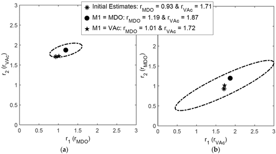 | ||
| Fig. 2 Influence of indexing the monomers on reactivity ratios and 95% JCI, reproduced from ref. 25 with permission. | ||
To avoid such mistakes entirely in the future we recommend that errors in the measurements be expressed in absolute numbers. If we take the absolute numbers based on the 10% error in F for the dataset of ref. 25 and, switch the index but use the same absolute errors for F, we get identical reactivity ratios and identical JCIs (see ESI-Fig. 1 and 2†).
Related to the indexing issue (see above) is how the estimation of the errors in the dependent variable is done and we will see that this in turn can influence the size of the JCI.
We would like to emphasize the importance of some knowledge of the error (structure) in the measured data. If there is a large variation in the size of the error within a dataset, the error can be used to weight the data in the fit.16
In many cases, monomer mixture composition data is obtained by integrating NMR spectra of the reaction mixture. In this situation, the intensity of the signals due to monomer decreases as the conversion increases, and an appropriate weighting function is given by eqn (9):26
 | (9) |
This function will be appropriate to other methods of determining monomer composition as a function of conversion in which the intensity of a signal is directly proportional to the amount of monomer present and so eqn (9) can be generally recommended for use.
In the event that the errors are known, for example through an error propagation exercise or through replicate measurements, the errors can be used to construct the joint confidence interval using the χ2 distribution27 with ss(r1,r2)z the boundary of the JCI at level z (for example a 95% probability):
| ss(r1,r2)z ≤ ssmin(r1,r2) + σ2χ2z(p) | (10) |
Here σ2 corresponds to the average absolute variance of the dependent variable (in this case F) and is calculated from the known errors as entered by the user. ssmin(r1,r2) is the sum of squares of residuals at the minimum and with p degrees of freedom (p equals two in the present cases).
4. The starting point of the calculation should not affect the estimates (this is in reference to the use of iterative methods to find the optimal values).
In general, in iterative methods the values of the optimum depend slightly on the starting point of the calculation.12 Luckily for determinations of reactivity ratios from the terminal copolymerization model there are no false minima. The VSSS method is not an iterative method, which means that even upon expansion to more complex models, falls minima will not be an issue.
5. Distortion of the error structure by linearization methods cannot be expected to give good estimates of the reactivity ratios.
While the copolymerization equation can be linearized using the Fineman–Ross,10 Kelen–Tüdős11 and other methods, doing so introduces bias into the results. In addition, these methods can only be used for low conversion data. We therefore strongly recommended to use NLLS, which provides an estimate of the reactivity ratios which is not biased by linearization.
In Fig. 3 we show the differences in output using the Fineman–Ross (F–R),10 Kelen–Tüdős (K–T)11 and NLLS14 methods applied to simulated data with noise. It can be seen that the F–R method is always liable to give poor results (compared to the true values), NLLS always gives good results, and the K–T is sometimes OK (left-hand figure), other times not (right).
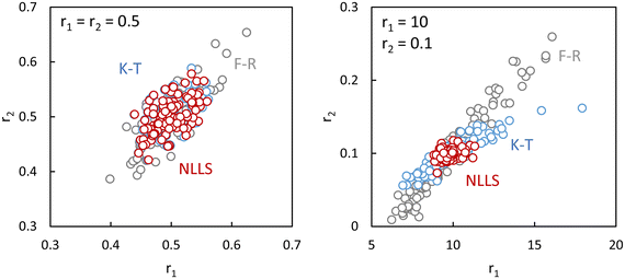 | ||
| Fig. 3 Differences using Fineman–Ross (F–R)10 and Kelen–Tüdős (K–T)11 and NLLS methods applied to simulated data with noise, where the true values are given in the upper left of each figure, and the circles are the values obtained from each analysis of simulated composition data with different noise (more details see ESI-Tables 1–3†). | ||
As the NLLS method does not involve any linearization, distorting the error structure is not an issue. However, it is important to stress that some knowledge of the errors in the measurements (error in copolymer composition F) is needed.
In the case that the errors are exactly known, the errors are also used to construct the JCI (eqn (10)). If the errors are only estimates (which is often the case), the JCI at level z is constructed through the following equation:
| ss(r1,r2)z ≤ ssmin(r1,r2)(1 + p/(n − p)Fz(p,n − p)) | (11) |
Another aspect that needs to be discussed with respect to errors is that statistics can only deal with random errors. As soon as systematic errors appear, the JCI will no longer give a useful reflection of reality. For example, if through a weighing error the true f0 is significantly different from the reported value, all the data from that experiment are systematically biased. For this reason, it is recommended that several different starting values for f0 are used (see also point 6). If each of these f0 sets (e.g. the different curves in Fig. 1) have different systematic errors, the overall fit with all the different f0 values and associated systematic errors is more likely to transpose to a random error. After all, if the source of the systematic error is for example a weighing error for f0, it might be expected that these weighing errors across the different f0 values are again randomly distributed. The sum of squares of residuals at the minimum will be larger than for the individual f0 sets and ssmin(r1,r2), through eqn (10) or (11) will increase the size of the JCI. We will address this issue in more detail in the paragraphs on systematic errors.
6. Correct design of experiments is of great importance.
Design of experiments can also be applied on the IUPAC recommended method. In the case of low conversion data, we recommend use of at least three different f0 values, where two of them can be chosen through the Tidwell–Mortimer D-optimal design criteria.22 Some estimate of the reactivity ratios is needed. We realize that the Tidwell–Mortimer approach is only applicable to low conversion experiments and cannot be extended to higher conversions. We are currently working on developing appropriate criteria for high conversion experiments. The third value (and other values) can be chosen on the basis of potential complications (e.g. complex formation between monomer and polymer, influence of high conversion).
7. Results should be reported as a point estimate together with a joint confidence interval.
Because we calculate the full sum of squares space in the VSSS approach, the unbiased joint confidence interval with exact shape for the parameter estimates is given as a contour line in the sum of squares space using eqn (10) or (11). Some software report the approximate JCI estimate in the form of an ellipse, see for example Fig. 2 and compare to ESI-Fig. 2 and 3† for unbiased joint confidence intervals (see ref. 15 for an extensive discussion on this topic). Reporting the JCI in some form is strongly recommended.
8. If there is also an error in the monomer composition (fi), the errors in (all) variables method (EVM) should be used, and this is especially relevant for the determination of reactivity ratios from conversion dependent data using the integrated copolymerization equation.
In the IUPAC recommended method (f0 − X − F) we measure the copolymer composition (or the monomer composition which is then converted into a copolymer composition using the mass balance in eqn (5)) and estimate the error in F. The error in X can either be transposed into an error in F (see for example ref. 16) or taken into account via the EVM.25 In the VSSS method, the EVM can also be applied.26. The errors in f0 have been discussed already with point 3.
The errors are important in three ways: (1) they can be used to weigh the data; (2) They determine the size of the JCI (in case of known errors and applying eqn (10); and (3) They can be used to determine whether the fit is adequate by comparing the actual fitting residues with the estimated errors (eqn (7)).
Besides these eight points, O'Driscoll also highlighted the “ease criterion”. The easier it is for the polymer chemist to apply a method to obtain reactivity ratios, the more likely it is that the method will be used. This is why our working group undertook to make free software available for applying the IUPAC recommended method as a stand-alone program (Contour),28 as open source Python code29 and as an Excel workbook with macro,30 all containing the VSSS method for f0 − X − F data. We recommend that either f0 − X − F (either directly measured F-values or converted from f) or (very) low conversion (f0 − F) data may be used.
Application of the IUPAC recommended method
We implemented the IUPAC method in the existing freeware Contour.14–16 There we used the VSSS method and f0, X, F, ΔF (absolute error in F) data. The software carries out numerical integration of the copolymerization equation during the parameter estimation process. This means that software issues due to singularities are minimized, but that calculation time can be a couple of seconds up to a few minutes. A JCI is generated, as well as a graphical display of the residuals in the 3-dimensional f0 − X − F plot. It is determined whether the fit is adequate by comparing the actual fitting residues with the estimated errors through a Fisher test (eqn (7)).We first generated a dataset with random noise (±0.005 on X and F) and original reactivity ratios of r1 = 0.4 and r2 = 0.6 (exact values), (see ESI-table 4†).
The resulting reactivity ratios are r1 = 0.401 ± 0.003 and r2 = 0.601 ± 0.003 (ESI-Table 4 and for the JCI SI-Fig. 3†).
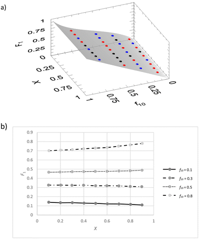
We see that the residuals space (Fig. 4a) shows an even distribution of positive, negative and even close to zero residuals. Of course, because this is a dataset with limited random errors added, this result is as expected.
We also used an experimental dataset from the group of Schmidt-Naake31 which is shown in Table 1:
We selected this experimental dataset because the necessary f0 − X − F data are directly available (not indirectly through f measurements) and this system might not behave according to the regular terminal model as acid–base interactions are expected between the APSA and the VIm.31
| f 10 | X | F 1 | ΔF1 |
|---|---|---|---|
| a f 10 initial ratio of APSA in the monomer mixture, X overall monomer conversion, F1 the content of APSA in the copolymer. | |||
| 0.05 | 0.04 | 0.404 | 0.030 |
| 0.05 | 0.093 | 0.381 | 0.030 |
| 0.05 | 0.209 | 0.316 | 0.030 |
| 0.05 | 0.195 | 0.282 | 0.030 |
| 0.05 | 0.279 | 0.227 | 0.030 |
| 0.05 | 0.434 | 0.146 | 0.030 |
| 0.1 | 0.1 | 0.458 | 0.030 |
| 0.1 | 0.182 | 0.457 | 0.030 |
| 0.1 | 0.194 | 0.407 | 0.030 |
| 0.1 | 0.301 | 0.396 | 0.030 |
| 0.1 | 0.389 | 0.347 | 0.030 |
| 0.1 | 0.474 | 0.235 | 0.030 |
| 0.3 | 0.109 | 0.547 | 0.030 |
| 0.3 | 0.168 | 0.491 | 0.030 |
| 0.3 | 0.201 | 0.484 | 0.030 |
| 0.3 | 0.383 | 0.486 | 0.030 |
| 0.3 | 0.456 | 0.488 | 0.030 |
| 0.3 | 0.731 | 0.467 | 0.030 |
| 0.7 | 0.068 | 0.658 | 0.030 |
| 0.7 | 0.186 | 0.654 | 0.030 |
| 0.7 | 0.274 | 0.677 | 0.030 |
| 0.7 | 0.332 | 0.642 | 0.030 |
| 0.7 | 0.482 | 0.635 | 0.030 |
| 0.7 | 0.577 | 0.649 | 0.030 |
| 0.7 | 0.739 | 0.658 | 0.030 |
| 0.9 | 0.13 | 0.872 | 0.030 |
| 0.9 | 0.273 | 0.856 | 0.030 |
| 0.9 | 0.43 | 0.83 | 0.030 |
| 0.9 | 0.585 | 0.915 | 0.030 |
| 0.9 | 0.71 | 0.91 | 0.030 |
| 0.9 | 0.82 | 0.88 | 0.030 |
With the IUPAC method the obtained reactivity ratios are 0.40 for r1 and 0.022 for r2 (see ESI-Table 5†) whereas in the original paper values of 0.31 for r1 and 0.026 for r2 were reported using a slightly different fitting procedure.31 Based on comparison of the estimated errors in F (0.030) with the actual fit residues it is determined that the terminal model gives an adequate fit to the data (ESI-Table 5†). The JCI is shown in Fig. 5.
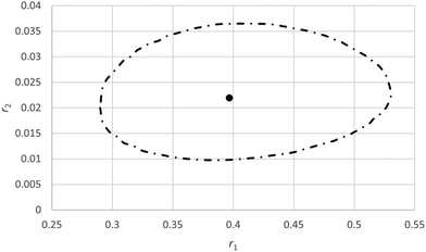 | ||
| Fig. 5 95% Joint confidence interval based on eqn (11) for the reactivity ratios of copolymerization of 2-acrylamido-2-methyl-1-propanesulfonic acid (APSA, monomer 1) and 1-vinylimidazole (Vim, monomer 2).29 | ||
As in this case it is expected that complexation between the two monomers will occur, some systematic trend in the residuals is expected. Schmidt-Naake et al.31 report that maximum complexation between the two monomers takes place at f10 of 0.5. We see that in the middle region most residuals are negative whereas at low f10 values most residuals are positive, indicating some systematic deviations (Fig. 6). Also it has to be noted that at low f10 values monomer 1 is depleted at higher conversions.
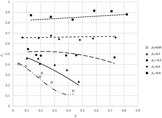 | ||
| Fig. 6 Plots of X, F1 data for the copolymerization of 2-acrylamido-2-methyl-1-propanesulfonic acid (APSA, monomer 1) and 1-vinylimidazole (Vim, monomer 2). | ||
The best way to investigate this further is by deleting some data structurally (e.g., take out low f0 values or high conversion data) from the set and see whether the reactivity ratios change. For example, if we take out the f10 = 0.05 and f10 = 0.1 data, we obtain 0.42 and 0.058 (ESI-Table 6†) for r1 and r2 respectively, more than doubling the value of r2.
Effect of systematic errors in the initial monomer fraction in copolymerization experiments
In order to investigate how sensitive an analysis of an f0 − X − F dataset is in errors in f0 we generated a dataset with little composition drift from reactivity ratios of r1 = 0.40 and r2 = 0.60 respectively and with initial monomer fraction (f10) of 0.1, 0.3, 0.5 and 0.8. We superimposed an absolute random error on both conversion (X) and cumulative copolymer composition (F1) of ± 0.005 each.In Fig. 7 the original reactivity ratios (triangle) and the fitted reactivity ratios with the noisy data (circle) are shown (r1 = 0.396 and r2 = 0.595) as well as the corresponding JCI's. Now we alternatingly added and subtracted 0.01 to the four f10 values given above (in modification 1 we added first, in modification 2 we subtracted first) to create a systematic error in each experiment starting from a (incorrectly determined) f10 value only. All the other measurements are assumed to only have a random error. With these new data the fit is obviously worse and the JCI is much larger (see Fig. 7), due to the poor fit and thus the sum of squares of residuals at the minimum increases (we used the Fisher-distribution for the JCI).
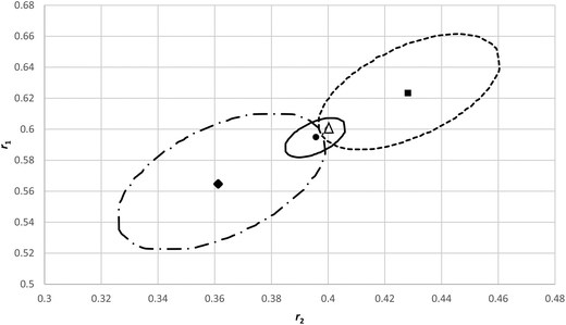 | ||
| Fig. 7 95% JCI's based on eqn (11) for original reactivity ratios r1 = 0.6 and r2 = 0.4 (Δ), with random errors added but without systematic errors in f10 (─) and with systematic errors in f10, modification 1 is adding/subtracting 0.01 with signs +−+− (----), modification 2 is −+−+(─ -). | ||
It is important to note that the minima can shift considerably and differently, depending on the systematic errors introduced on the original f10 values. Although the 95% JCI's are much bigger, they barely touch the correct values. The systematic errors introduced in f10 in the individual experiments, overall seen over the different f10 values, are more or less random (2 × +0.01, and 2 × −0.01), but it makes a difference how we apply them (modification 1 vs. modification 2).
We plotted the residuals for the data (modification 1 in Fig. 7), which clearly indicate systematic deviations per experiment (see ESI- Fig. 6†).
This means that particular care has to be taken to avoid an error in the f10 values, but a residuals plot (like Fig. 4a) can be used to identify such issues. However, if we only take a single experiment with the systematic errors included, we obtain reactivity ratios diverging significantly from the true values with very large JCI's. It is an option to vary f10 values in a single experiment and see how the quality of the fit improves. This approach is recommended as very small variations in f10 have a major influence on the SSR and on the obtained reactivity ratios in for example X vs. f data (see ESI-Fig. 8†).
We also investigated a system with more composition drift and reactivity ratios of r1 = 13 and r2 = 0.3 (ESI-Fig. 5–7†). Applying systematic errors in f10 again, like we did before, there is hardly any overlap of the JCI's (ESI-Fig. 7†). If we use a single experiment (one f10) with systematic error, hugely incorrect reactivity ratios are likely to be obtained. However, by taking a series of different f10 experiments we can still obtain reasonable estimates for the reactivity ratios. However, the JCI's with systematic errors seem to be not large enough to overlap with the true reactivity ratios (ESI-Fig. 7†). The increase in JCI due to a larger sum of squares of residuals at the minimum is not sufficient to reflect the increased error in the reactivity ratios. One of the assumptions in the non-linear least squares method is that the errors are independent, which is obviously violated here within a single experiment starting from a wrong f10 value.
The conclusion is that errors in the value of f10 should be avoided at all costs. One option is to investigate the residuals space and see whether there is a systematic pattern in one or more of the experiments starting from a particular f10. If that is the case, an error in f10 could be assumed and a correction could be made by varying f10 and looking for the best value (see ESI-Fig. 8†). These variations in f10 could be as small as ±0.002, so usually well within the estimated error range for f. This option is available in Contour, with the optimized f10 value suggested by the software then used to see if the overall fit improves.
Recommendations
-Use only non-linear regression or VSSS methods.-Either use low conversion f0 − F data or conversion dependent data in the form of f0 − f − X or f0 − X − F, in all cases with at least three different starting monomer compositions f0.
-If using low conversion f0 − F data, check that no significant (more than the expected random error) change in F has occurred due to composition drift. Once the reactivity ratios are estimated, the predicted change in F with conversion should then be calculated. If this indicates too much composition drift over the range of X used experimentally, then one should go back and use the f0 − X − F method instead.
-Obtain the best possible information about the errors in the measurements, and utilize weighting according to the errors in the dependent variable (in most cases F).
-If the independent variable (usually f) has considerable error, use EVM.
-If using f0 − f − X data without EVM, convert the f0 − f − X data into f0 − X − F with proper error propagation, taking errors in f (also f0 if needed) and X into account.
-Be aware of errors in f0, especially in conversion dependent experiments.
-Mitigate errors in f0 through (1) measuring f0 (e.g. through NMR), and/or (2) investigating limited variations in f0 though fitting f0 − f − X single experiments, and/or (3) looking at the residuals in a set of experiments and detecting systematic patterns (if so, vary f10 again).
-Analyse the residuals and compare the fit residuals with the estimated errors.
-Investigate if fit residuals exceed the expected errors; if they do, this usually indicates either that the terminal model is not valid for the copolymerization system under investigation and/or that systematic errors are present.
-The obtained reactivity ratios should be reported with the correct number of significant digits (typically 2) and a measure of the uncertainty in those values (preferably a joint confidence interval).
Conclusion
The IUPAC working group on “Experimental Methods and Data Evaluation Procedures for the Determination of Radical Copolymerization Reactivity Ratios” has established a robust method to determine reactivity ratios from composition data following the terminal model. The method is based on measuring conversion (X) and (cumulative) copolymer composition (F) in a few copolymerization reactions at different starting monomer compositions (f0), although a set with only low conversion can also be used (f0 − F). Importantly, we make freely available the analysis software for this method, and we strongly recommend that it be used for reactivity ratio determination. The method not only provides parameter estimates but can also reveal deviations from the terminal model and systematic errors in the dataset. It is shown that error estimation for the F-values is important for weighing the data, determining the size of the joint confidence interval (in case of accurately known errors) and discerning whether the fit with the terminal model is adequate. In principle previous experiments measuring f0 − F (if conversion is known or sufficiently low) can still be analyzed with the IUPAC recommended method. Some examples have been given of reactivity ratio determinations, both with experimental data as well as simulated data. Special attention has been given to the occurrence of systematic errors in the f0 − X − F and f0 − f − X experiments. It is shown that the current statistical treatment is not able to properly accommodate systematic errors occurring within such experiments. However, with the analysis of the residuals space (f0 − X − F) these errors can be identified and where possible corrected through optimization of f0 as a third parameter.The design of experiments procedure for the recommended method is under development.
Author contributions
Anton A. A. Autzen: investigation, methodology, writing – review & editing; Sabine Beuermann: investigation, methodology, writing – review & editing; Marco Drache: investigation, methodology, writing – review & editing; Christopher M. Fellows: investigation, methodology, writing – review & editing; Simon Harrisson: investigation, methodology, project administration, writing – review & editing, software, formal analysis, funding acquisition; Robin A. Hutchinson: investigation, methodology, writing – review & editing; Atsushi Kajiwara: investigation, methodology, writing – review & editing; Daniel J. Keddie: investigation, methodology, writing – review & editing; Bert Klumperman: investigation, methodology, writing – review & editing, software; Gregory T. Russell: conceptualization, investigation, methodology, writing – review & editing; Alex M. van Herk: investigation, methodology, project administration, writing – original draft, software, formal analysis, funding acquisition.Conflicts of interest
No conflicts of interest.Acknowledgements
We would like to acknowledge Dr Robert Reischke (Postdoctoral Fellow at AIfA Bonn) for valuable discussions. We also thank the International Union of Pure and Applied Chemistry (IUPAC) for financial support (Project No. 2019-023-1-400).32References
- S. Penczek and G. Moad, Pure Appl. Chem., 2008, 80, 2163–2193 CrossRef CAS.
- J. P. A. Heuts, R. G. Gilbert and I. A. Maxwell, Macromolecules, 1997, 30, 726–736 CrossRef CAS.
- B. S. Beckingham, G. E. Sanoja and N. A. Lynd, Macromolecules, 2015, 48, 6922–6930 CrossRef CAS.
- G. E. Roberts, M. L. Coote, J. P. A. Heuts, L. M. Morris and T. P. Davis, Macromolecules, 1999, 32, 1332–1340 CrossRef CAS.
- J. Zhang, B. Farias-Mancilla, M. Destarac, U. S. Schubert, D. J. Keddie, C. Guerrero-Sanchez and S. Harrisson, Macromol. Rapid. Commun., 2018, 39, 1800357 CrossRef PubMed.
- R. A. Hutchinson, B. Klumperman, G. T. Russell and A. M. Van Herk, Can. J. Chem. Eng., 2022, 100, 680–688 CrossRef CAS.
- F. R. Mayo and F. Lewis, J. Am. Chem. Soc., 1944, 66, 1594–1601 CrossRef CAS.
- I. Skeist, J. Am. Chem. Soc., 1946, 68, 1781–1784 CrossRef CAS PubMed.
- V. E. Meyer and G. G. Lowry, J. Polym. Sci., Part A: Gen. Pap., 1965, 3, 2843–2851 CrossRef CAS.
- M. Fineman and S. D. Ross, J. Polym. Sci., 1950, 5, 259–265 CrossRef CAS.
- T. Kelen and F. Tüdős, React. Kinet. Catal. Lett., 1974, 1, 487–492 CrossRef CAS.
- K. F. O'Driscoll and P. M. Reilly, Makromol. Chem., Macromol. Symp., 1987, 10/11, 355–374 CrossRef.
- M. Dube, R. Amin Sanayei, A. Penlidis, K. F. O'Driscoll and P. M. Reilly, J. Polym. Sci., Part A: Polym. Chem., 1991, 29, 703–707 CrossRef CAS.
- A. M. van Herk, J. Chem. Educ., 1995, 72, 138–140 CrossRef CAS.
- A. M. van Herk and T. Dröge, Macromol. Theory Simul., 1997, 6, 1263–1276 CrossRef CAS.
- M. Buback, T. Dröge, A. M. van Herk and F. O. Mähling, Macromol. Chem. Phys., 1996, 197, 4119–4134 CrossRef CAS.
- R. Reischke, Macromol. Theory Simul., 2023, 32, 202200063 CrossRef.
- J. B. Lena and A. M. van Herk, Ind. Chem. Eng. Res., 2019, 58, 20923–20931 CrossRef CAS.
- S. M. Shawki and A. E. Hamielec, J. Appl. Polym. Sci., 1979, 23, 3155–3166 CrossRef CAS.
- C. Preusser and R. A. Hutchinson, Macromol. Symp., 2013, 333, 122–137 CrossRef CAS.
- R. E. Cais, R. G. Farmer, D. J. T. Hill and J. H. O'Donnell, Macromolecules, 1979, 12(5), 835–839 CrossRef CAS.
- P. W. Tidwell and G. A. Mortimer, J. Polym. Sci., Part A: Gen. Pap., 1965, 3, 369–387 CrossRef CAS.
- R. A. Sanayei, K. F. O'Driscoll and B. Klumperman, Macromolecules, 1994, 27, 5577–5582 CrossRef CAS.
- S. K. Fierens, P. H. M. Van Steenberge, M.-F. Reyniers, D. R. D'hooge and G. B. Marin, React. Chem. Eng., 2018, 3, 128–145 RSC.
- A. J. Scott and A. Penlidis, Processes, 2018, 6, 8, DOI:10.3390/pr6010008.
- M. van den Brink, A. M. van Herk and A. L. German, J. Polym. Sci., Part A: Polym. Chem., 1999, 37, 3793–3803 CrossRef CAS.
- P. J. Rossignoli and T. A. Duever, Polym. React. Eng., 1995, 3(4), 361–395 CAS.
- A. M. van Herk, Software package Contour issue 2.4.0, accessed 03/04/2024 https://drive.google.com/file/d/1lYicEcPbuQiohQGE4x5RUVALTVU9sWnL/view?usp=sharing Search PubMed.
- Code in Python for the VSSS method applied on f0 − X − F data, accessed 02/04/2024 https://drive.google.com/file/d/1a_Co9-hULovu0ns5rcVoancyG3IyeXU0/view?usp=sharing.
- Code in Excel (via VB) for the VSSS method applied on f0-X-F data, accessed 02/04/2024 https://drive.google.com/file/d/1TnqnuVSmp5EcHLqia5OI5BZx_3pMHAsE/view?usp=sharing.
- C. Schmidt, F. Merz, S. Jiang, M. Drache and G. Schmidt-Naake, Macromol. Mater. Eng., 2007, 292, 428–436 CrossRef CAS.
- IUPAC project site, last accessed 03/03/2024 https://iupac.org/project/2019-023-1-400/.
Footnote |
| † Electronic supplementary information (ESI) available. See DOI: https://doi.org/10.1039/d4py00270a |
| This journal is © The Royal Society of Chemistry 2024 |

