
 Open Access Article
 This Open Access Article is licensed under a Creative Commons Attribution-Non Commercial 3.0 Unported Licence
Impact of excitation pulse width on the upconversion luminescence lifetime of NaYF4:Yb3+,Er3+ nanoparticles†
Alejandro
Casillas-Rubio
 a,
Diego
Mendez-Gonzalez
b,
Marco
Laurenti
b,
Jorge
Rubio-Retama
b,
Oscar G.
Calderón
*a and
Sonia
Melle
*a
a,
Diego
Mendez-Gonzalez
b,
Marco
Laurenti
b,
Jorge
Rubio-Retama
b,
Oscar G.
Calderón
*a and
Sonia
Melle
*a
aDepartment of Optics, Complutense University of Madrid, E-28037 Madrid, Spain. E-mail: oscargc@ucm.es; smelle@fis.ucm.es
bDepartment of Chemistry in Pharmaceutical Sciences, Complutense University of Madrid, E-28040 Madrid, Spain
First published on 17th May 2024
Abstract
The upconversion luminescence (UCL) lifetime has a wide range of applications, serving as a critical parameter for optimizing the performance of upconversion nanoparticles (UCNPs) in various fields. It is crucial to understand that this lifetime does not directly correlate with the decay time of the emission level; rather, it represents a compilation of all the physical phenomena taking place in the upconversion process. To delve deeper into this, we analyzed the dependence of the UCL lifetime on the excitation pulse width for β-NaYF4:Yb3+,Er3+ nanoparticles. The results revealed a significant increase in the UCL lifetime with both the excitation pulse width and the excitation intensity. The laser fluence was identified as the parameter governing the UCL decay dynamics. We showcased the universality of the pulse-width-dependent UCL lifetime phenomenon by employing UCNPs of various sizes, surface coatings, host matrices, Yb3+ and Er3+ ratios, and dispersing UCNPs in different solvents. Theoretical explanations for the experimental findings were derived through a rate equation analysis. Finally, we discussed the implications of these results in UCNP-FRET (Förster resonance energy transfer)-based applications.
1 Introduction
Nanocrystals doped with rare-earth ions exhibit unique photoluminescent properties, owing to their unique ability to facilitate photon upconversion—a nonlinear optical phenomenon that transforms lower-energy photons into higher-energy photons.1 Additionally, upconversion nanoparticles (UCNPs) exhibit significant anti-Stokes shifts, absence of photobleaching and photoblinking, long luminescence lifetimes, narrow emission bands, and emission wavelength tuning capacity. These distinctive characteristics render them highly attractive materials for a wide range of applications, including bioimaging,2,3 sensing,4–6 theranostics,7 anti-counterfeiting,8 solar cells,9,10 small drug delivery systems,11 or nanothermometry,12–14 underscoring their remarkable scientific and technological potential.UCNPs consist of a low-phonon-energy matrix, such as NaYF4 (phonon energy 300–400 cm−1),15 where usually two different rare-earth ions are embedded, one acting as a sensitizer and the other as an activator. Within these pairs of ions, Yb3+ and Er3+ are among the most commonly used as sensitizers and activators, respectively, due to the ability of Yb3+ ions to absorb excitation photons at 980 nm and transfer the energy to Er3+ ions. Successive energy transfer steps populate higher energy levels of Er3+, and upon radiative relaxation, release higher energy photons, spanning multiple bands across the UV and visible regions of the electromagnetic spectrum.16
The temporal response of upconversion luminescence (UCL), and particularly the UCL lifetime, stands out as a crucial parameter for UCNP-based technologies and as a fundamental feature for characterizing the emission performance of UCNPs. Recently, some studies have brought attention to the complex nature of the time-related behavior of UCL, suggesting the need to revisit this subject.17 Although the luminescence decay time has traditionally been ascribed solely to the intrinsic lifetime of the emitting state, the UCL lifetime is a reflection of the temporal response of the entire upconversion process. For instance, Chai et al. showed that the green UCL lifetime from Er–Yb-codoped UCNPs changes significantly when the Yb3+ sensitizer excited state is quenched by fluorophores loaded onto the nanoparticle surface.18 In this vein, Bergstrand et al. demonstrated that the UCL lifetime of Er–Yb-codoped nanorods only approaches the intrinsic lifetime of the emitting state when the sensitizer's excited state has a significantly shorter lifetime and there are no cross-relaxation processes involving the emitting energy level.19 Various kinetic models have been proposed to accurately fit the UCL decay curves, enabling the extraction of information related to various involved processes.20
The intricate temporal dynamics displayed by UCNPs appear to challenge a fundamental axiom of luminescence lifetime: the assumption that luminescence lifetime remains unaffected by excitation. Indeed, power-dependent UCL lifetime has been reported.21–24 Different relationships between UCL lifetime and laser power have been found, depending on several factors such as the nanoparticles’ size and structure (core vs. core–shell), excitation irradiance range, composition of doping ions in the nanoparticles, as well as whether powder or solutions are used. For instance, Han et al.22 observed an increase in UCL lifetime for powder NaLuF4:Yb0.9,Er0.02 microrods when increasing excitation power from 3 W cm−2 to 25 W cm−2 using pulses up to 1 ms width. However, single nanoparticle experiments using NaYF4:Yb0.2,Er0.02@NaYF4 nanoparticles with different sizes showed that the lifetime decreases with excitation power for particles with diameters greater than 30 nm, reaching a saturation for 105–107 W cm−2, while the lifetime of smaller particles did not show any variation with excitation power.23 On the other hand, Teitelboim et al.24 reported that the UCL lifetime of core@shell NaYF4:Yb0.2,Er0.02@NaYF4:Gd0.2 was relatively independent of excitation power with 4 ms pulses, but when increasing Er3+ doping, the power increments resulted in a reduction in UCL lifetime. As Teitelboim et al. stated,24 the power dependency of UCL lifetime arises from the initial distribution of excited-state populations of active ions at the onset of luminescence decay. This distribution is set by excitation power and determines energy transfer rates, indicating that decay kinetics is a history-dependent phenomenon.
By controlling the excitation pulse width, Han et al. have modulated the UCL dynamics.22 They showed a huge variation (20-fold) in the 540 nm UCL lifetime of Er3+ in microrods of NaLuF4:Yb0.9,Er0.02. Recently, Gao et al.25 reported an increase in the green emission lifetime with pulse width of 78% for 20 nm NaYF4:Yb0.05,Er0.02 nanoparticles demonstrating that particles shielded from the environment with an inert NaYF4 shell exhibit a much milder variation in lifetime (12%) compared to ligand-free particles (267%). They also observed that nanoparticles with higher Yb3+ content and lower Er3+ content exhibit lesser changes in lifetime with pulse width.
All this novel knowledge has a great impact, as UCL lifetime measurements are broadly used for multiple applications, such as in Förster Resonance Energy Transfer (FRET)-based UCL sensors. Typically, in such systems, the formation of a complex between the analyte (acceptor) and the UCNP (donor) leads to a change in the FRET efficiency, which is transduced into a variation of the fluorescence emission of both acceptor and donor. Besides that, the FRET process is accompanied by a modification of the UCL lifetimes of the donors. This property arises from the different radiative and non-radiative processes involved, with the FRET process acting as a new energy transfer pathway. Therefore, minimizing the occurrence of other non-radiative energy transfer pathways could maximize the FRET contribution to the resulting UCL lifetime.26,27 Interestingly, this effect could introduce a bias in FRET-based sensors, resulting in significant variations in UCL intensity accompanied with minimal modifications in UCL lifetime.27 For this reason, these three factors (distance, number and nature of energy transfer pathways) have been extensively studied to optimize the performance of FRET sensors.28 Strikingly, the variation of the UCL lifetime can also be affected by the excitation pulse width, which needs to be studied and understood. For instance, Kotulska et al. explored the performance of a FRET-based UCL sensor using NaYF4:Yb0.2,Er0.02 UCNPs as donors and Rose Bengal as the acceptor, employing various excitation schemes.29 They found that short excitation pulses (5–7 ns) could yield more sensitive assays compared to long excitation pulses (4 ms).
Our aim in this work is to gain a more profound understanding of how the excitation pulse width and power influence the UCL decay dynamics. To do that, we used NaYF4:Yb0.2,Er0.02 UCNPs coated with a protective hydrophobic polymer shell. We performed a parametric analysis, exploring the variation in the UCL lifetime of the emission bands by changing the excitation pulse width from the microsecond range to the millisecond range. Furthermore, we investigated the influence of both laser power and spot size in the UCL lifetime, exploring their relationship with the pulse width. Additionally, we employed various types of UCNPs by modifying the host matrix, doping concentration of rare-earth ions, surface coating, and solvent. In all cases, a consistent relationship between the UCL lifetime and the excitation pulse width was observed. These results were modeled using a rate equation analysis, which allowed us to explore the role of the initial population of the excited states in the UCL decay dynamics. Finally, we discuss some implications of the excitation-dependent UCL lifetime on UCNP-FRET-based applications.
2 Experimental section
2.1 Chemicals
Yttrium(III) chloride hexahydrate (YCl3·6H2O, 99.99%), ytterbium(III) chloride hexahydrate (YbCl3·6H2O, 99.9%), erbium(III) chloride hexahydrate (ErCl3·6H2O, 99.9%), 1-octadecene (ODE, 90%), oleic acid (OA, 90%), oleylamine (OLA, 70%), sodium hydroxide (98%), ammonium fluoride (98%), n-hexane (95%), methanol (99.9%), dimethyl sulfoxide (DMSO, ≥99.9%), chloroform (CHCl3, ≥99.8%), N,N-dimethylformamide (DMF, >99%), nitrosyl tetrafluoroborate (NOBF4, 95 mol), ethanol absolute (EtOH), n-hexane (97%), yttrium(III) oxide (Y2O3, 99.9%), ytterbium(III) oxide (Yb2O3, 99.9%), erbium(III) oxide (Er2O3, 99.9%), thulium(III) oxide (Tm2O3, 99.9%), trifluoroacetic acid (TFA, 99%), calcium carbonate (CaCO3, 99.99%), strontium carbonate (SrCO3, 99.9%), tetraethylorthosilicate (TEOS), and igepal co-520 were purchased from Sigma-Aldrich (Merck). 10-Methacryloyldecylphosphate (MDP, 99%) was purchased from LGC Group, Spain. All chemicals were used as received without further purification.2.2 Synthesis of NaYF4:Yb3+,Er3+ UCNPs
The synthesis of β-NaYF4:Yb0.2,Er0.02 was performed following the protocol published in ref. 30. Briefly, a thermal co-precipitation method was used to obtained monodisperse UCNPs with a mean diameter of 36 ± 1 nm. The subsequent treatment of UCNPs with NOBF4 removed from their surface the oleate molecules, which acted as a capping agent, allowing the phase transfer of the resulting UCNPs from hexane to N,N-dimethylformamide (DMF). Their later incubation with 10-methacryloyldecylphosphate (MDP) in DMF/CHCl3 resulted in their surface functionalization with MDP. Miniemulsion polymerization was used to cover the resulting UCNPs–MDP with a protective hydrophobic polymer shell. In this method, a mixture of 75% styrene (St) and 25% methyl methacrylate (MMA) formed the dispersed oily phase, sodium dodecyl sulfate (SDS) was used as the surfactant, hexadecane was used as the hydrophobe or droplet co-stabilizer; and potassium persulfate (KPS) was used as the radical initiator. Details of the miniemulsion polymerization procedure are described in ref. 30. The final size of the UCNPs covered with the hydrophobic polymer shell, β-NaYF4:Yb0.2,Er0.02@PS/PMMA, is 58 nm.2.3 Characterization
The current laser controller is able to run the laser in CW mode for steady-state luminescence measurements. Additionally, it can generate light excitation pulses ranging from 40 μs to the millisecond range. The rise and fall time for the laser is much lower (nominal value lower than 10 μs) than the measured UCL decay times. The photomultiplier tube that collects the luminescence signal is connected to a 50 ohm input of a digital oscilloscope (Agilent, DSO9104A). The signal from the current laser controller serves as the trigger for the oscilloscope. A program developed in Matlab is employed to analyze each signal obtained in real time directly from the oscilloscope. This code can simulate the discriminator and the multichannel counter.32 After analyzing more than 5000 trigger signals, a luminescence decay curve is obtained. The luminescence lifetime was determined by fitting the decay curves to a single exponential function. For the fitting process, we considered a time window from tini to tend, with the final fitting time tend set long enough to allow the complete decay of luminescence (typically tend = 2–2.5 ms). For each experimental decay curve, we performed around 25 fits, varying the initial fitting time tini within the range where the luminescence signal intensity varies from 75% to 50% of its maximum value (additional details can be found in section S1 of the ESI in ref. 33). This fitting procedure provides an average lifetime with its standard error.
To characterize the laser intensity or irradiance at the sample, we measured the laser power with a thermal sensor power meter (Thorlabs, S310C) and the beam size using the knife-edge technique.34
3 Results and discussion
We used the thermal co-precipitation method at high temperature to synthesize quasi-spherical monodisperse β-NaYF4:Yb0.2,Er0.02 nanoparticles with a mean diameter of 36 ± 1 nm. An HR-TEM magnification of an oleate-capped UCNP is shown in Fig. S1A in the ESI,† showing the 100-lattice plane from the NaYF4 hexagonal phase. Furthermore, Selected Area Electron Diffraction (SAED) analyses confirmed the hexagonal β-phase according to the card JCPDS 16-0334 (see SAED pattern in section S1 in the ESI†). The resulting UCNPs were coated with a protective polymer shell as a way to transfer them to water, while avoiding luminescence quenching and degradation processes in this medium. This is particularly crucial when using them in biological applications, where the diffusion of water and other potential ligands can have detrimental effects on their optical properties due to water quenching35 and chemical degradation.36,37 Therefore, aiming to initially study the UCNPs’ lifetime behaviour in this biomedically relevant medium, but with the goal of ensuring the reliability and robustness of these results, we coated the UCNPs with a hydrophobic polymer shell through miniemulsion polymerization of styrene and methyl methacrylate, providing greater stability and structural integrity, as recently reported.30 It has been shown that the lifetime in these UCNPs remains unaffected by the environment over time.30 TEM image analysis of the resulting UCNPs showed a final diameter of the polymer-coated nanoparticle of 58 nm (Fig. 1A). Fig. 1B shows the green UCL emission spectrum of an aqueous NaYF4:Yb,Er UCNP dispersion (200 μg mL−1 concentration used in all the reported experiments) upon excitation with a 967 nm CW laser. This emission comprises two peaks at approximately 525 nm and 540 nm, corresponding to transitions 2H11/2 → 4I15/2 and 4S3/2 → 4I15/2, respectively (see the energy-level scheme of the system depicted in Fig. 1C, which includes the green upconversion process primarily driven by energy transfer (ET) from Yb3+ ions to Er3+ ions). | ||
| Fig. 1 (A) TEM image of 36 nm β-NaYF4:Yb0.20,Er0.02 nanoparticles coated with a hydrophobic polymer shell through miniemulsion polymerization of styrene (St) 75%, and methyl methacrylate (MMA) 25% mixture, β-NaYF4:Yb0.20,Er0.02@PS/PMMA. Final diameter of the polymer-coated nanoparticle: 58 nm. (B) Green UCL spectrum of an aqueous β-NaYF4:Yb0.20,Er0.02@PS/PMMA UCNP dispersion (200 μg mL−1) and excitation laser spectrum for a CW laser power of 0.3 W. (C) Energy-level diagram for Yb3+ and Er3+ ions describing the processes that give rise to green UCL emission bands. Black dashed lines represent the Yb–Er energy transfer (ET) mechanism, whereas green solid lines represent the two green emissions centered around 525 nm and 540 nm. | ||
Next, we analyzed the impact of the excitation pulse duration on the UCL lifetime of the UCNPs. The setup for conducting time-resolved luminescence experiments is illustrated in Fig. 2A. We measured the UCL decay curve of the green band (at 540 nm, with a monochromator nominal spectral bandwidth of less than 5 nm) by varying the pulse width of the NIR excitation laser (967 nm) across a range from a few microseconds to tens of milliseconds, both below and above the typical UCL lifetimes. The pulse repetition frequency was selected to ensure that the ions relax to the ground level before initiating the subsequent excitation pulse (see values in section S2 of the ESI†). The decay curves presented in Fig. 2B provide clear evidence of the dependency of the UCL lifetime on the pulse duration. Interestingly, increasing the excitation pulse width results in a corresponding increase in the UCL lifetime. Fig. 2C displays two representative configurations: a long excitation pulse of 1 ms (upper scheme) and a short excitation pulse of 40 μs (lower scheme). In the former case, the UCL decay curve clearly exhibits slower decay dynamics, giving a UCL lifetime of 207 μs, while shorter excitation pulses, 40 μs, result in quicker decays (147 μs). The UCL lifetime was determined by fitting the decay curves to an exponential function with a varied fitting window, as detailed in section 2. Additionally, we explored fitting the decay curves with a combination of exponential functions and calculating the weighted average of the obtained decay times. This approach yielded similar lifetime values (see section S3 in the ESI† for more details). To ensure that the observed variation in the UCL lifetime with the laser pulse width is not attributed to temperature-related factors, we conducted time-resolved luminescence experiments using a temperature-controlled cuvette holder. We measured the UCL decay curves as a function of the laser pulse width at two different temperatures, 20 °C and 40 °C, revealing a remarkably similar behavior (see section S4 in the ESI†). This experiment highlights the reproducibility of this phenomenon, even at different temperatures.
 | ||
| Fig. 2 (A) Schematic of the experimental setup to measure the time-resolved UCL. L1: collimating lens; Di: long-pass dichroic filter; 10×: microscope objective; F1: band-pass filter; L2: focusing lens; OF: optical fiber; PMT: photomultiplier tube; CC: coaxial cable. (B) Green (540 nm) UCL decay curves for different excitation pulse widths and a laser power of 2.2 W. (C) Two extreme representative cases depict the temporal evolution of the excitation pulse (40 μs and 1 ms) alongside the corresponding experimental UCL decay signal. (D) Green UCL lifetime as a function of the excitation pulse width for three different laser powers. Symbols are the experimental data and solid lines are the simulated results obtained by numerically solving eqn (1). (E) (left axis) UCL lifetime versus the distance from the excitation beam waist to the cuvette. Symbols are the experimental data and the solid line is the simulated result obtained by numerically solving eqn (1). (right axis) Laser spot size as a function of the cuvette position. The excitation pulse width was 5 ms, and the power was 2.2 W. (F) UCL lifetime from graphs (D) and (E) as a function of the laser fluence. The inset summarizes the analyzed excitation characteristics, including pulse width, power, and spot size. | ||
In order to further understand this phenomenon, we studied the behaviour of the UCL lifetime not only by varying the pulse width, but also the laser excitation power. Fig. 2D shows the UCL lifetime as a function of the laser pulse width for three different laser powers. As seen in the figure, the UCL lifetime increases with the laser power, a phenomenon that seems particularly relevant at long excitation pulses. This behavior agrees with previous reports.22,24 It is noteworthy that small UCNPs (8 nm) with high Er3+ concentrations,24 or single UCNPs (≥30 nm),23 appear to exhibit the opposite behavior, i.e., a reduction of UCL lifetime with increasing power. This has been attributed to a depopulation of the emitting states by power-dependent increased relaxation rate due to an increase in the spatial density of populated Er3+ excited states, which in turn increases the rates of ET and cross-relaxation out of these states. Hence, not only does the laser pulse width impact the measured green UCL lifetime, but so does the laser power. These results are particularly interesting, as they show two new parameters (pulse width and laser power) for controlling the time evolution of the UCL, and highlight how the combination of large laser pulses and increasingly higher excitation powers results in significant lifetime changes for UCNPs with a fixed chemical composition (Yb3+/Er3+ ratio and host matrix), nanoarchitecture, surface coating and surrounding environment.
To elucidate the interplay between excitation power and excitation pulse width in shaping the lifetime behavior, we measured the UCL decay curve by varying the position of the cuvette along the beam propagation axis while keeping a constant excitation pulse width (5 ms) and power (2.2 W). This allowed us to analyze the effect that the change of the laser beam size at a fixed pulse width and power had on the UCL lifetime. The laser beam diameter was firstly measured along the propagation axis using the knife-edge technique34 (see section S5 in the ESI† for more details). The UCL lifetime results are presented in Fig. 2E, left axis. The longest UCL lifetimes were achieved when the sample was placed at the beam waist (see laser spot diameter on Fig. 2E, right axis). As we exposed the sample to a larger beam size, the UCL lifetime decreased. These findings suggest that the variation in UCL lifetime is highly dependent on the optical energy per unit area, i.e., the laser fluence. To support this observation, we compiled all the previous lifetime measurements from Fig. 2D and E and plotted them in Fig. 2F as a function of laser fluence. It is noteworthy that our results reveal how all UCL lifetime data collapse into a single curve when represented in terms of laser fluence, demonstrating that this is the variable responsible for the observed lifetime behaviour.
These results give us important information about the role of the excitation pulse in establishing the population of the different energy states. The laser irradiance (I) controls the excitation rate, quantifying the number of excited Yb3+ ions per unit of time, whereas the laser fluence, on the other hand, signifies the overall number of excitation processes taking place during the excitation pulse. Consequently, the laser fluence governs the distribution of the population, just when the laser is turned off, among the various energy levels of the Er3+ and Yb3+ ions involved in the upconversion process. All of these factors suggest that the temporal behavior of the UCL decay is a history-dependent phenomenon.24,27,29
3.1 Theoretical interpretation
To investigate the experimentally observed phenomenon, we performed a rate equation analysis. Our aim was to replicate the behavior of the experimentally determined green UCL lifetime and to better understand the mechanisms behind it by using the rate equation model presented below: | (1) |
Here NErj is the density of Er3+ ions in the energy level j, where the subscripts j = 0, 1, 2, 3, and 4 represent the 4I15/2, 4I13/2, 4I11/2, 4F9/2, and 4S3/2 energy levels of Er3+ ions, respectively (see Fig. 3A). The population of fast-decaying levels as 4F7/2 and 4I9/2 are neglected and the populations of energy levels 2H11/2 and 4S3/2 are considered in thermal equilibrium. Therefore NEr0 + NEr1 + NEr2 + NEr3 + NEr4 = NEr, where NEr represents the total density of Er3+ ions in the nanoparticle. On the other hand, NYb0 and NYb1 are the Yb3+ ions density in the 2F7/2 and 2F5/2 energy levels, respectively (NYb0 + NYb1 = NYb, with NYb being the total density of Yb3+ ions in the nanoparticle). WErjl is the decay rate from Er3+ level j to level l, whereas WErj (WYbj for Yb3+ ions) is the total decay rate of the energy level j of Er3+ ions. The decay rates from an excited level to the ground state are considered radiative decay rates (in the millisecond range), while the decay rates from an excited level to the next lower excited level are considered faster nonradiative decay rates (in the microsecond range) due to multi-phonon relaxation. On the other hand, K2 and K4 are the coefficients of the resonant energy transfer from the excited Yb3+ ion (sensitizer) to levels 2 and 4 of the Er3+ ion (activator), respectively. KB2 is the coefficient of back energy transfer from the Er3+ ion in level 2 to the Yb3+ ion. CEr1 and CEr2 are the coefficients of cross-relaxation energy transfer between two neighboring Er3+ ions. CEr1 is the typical quenching mechanism that takes place in erbium-doped fiber amplifiers (4I13/2, 4I13/2) → (4I15/2, 4I9/2) and CEr2 is an upconversion energy transfer to the green-emitting level (4I11/2, 4I11/2) → (4I15/2, 4F7/2). The excitation laser intensity or irradiance is denoted as I (in units of W cm−2). This can be normalized by the saturation intensity Isat = ħωWYb1/(2σYb1) of the Yb3+ transition, where σYb1 is the corresponding absorption (≃emission) cross-section at the laser wavelength and ħω is the corresponding transition energy (resonant with the laser wavelength at 967 nm).
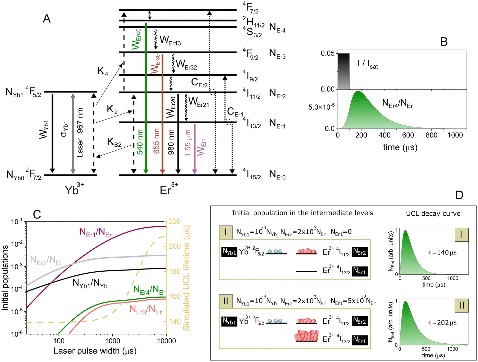 | ||
| Fig. 3 (A) Energy-level diagram for Yb3+ and Er3+ ions describing all the physical processes used in the rate equation model. Black dashed lines represent the Yb–Er ET mechanism (K2, KB2, and K4), whereas black dotted lines represent Er–Er ET mechanisms (CEr1 and CEr2). The gray solid line represents ground-state absorption (and stimulated emission) of Yb3+ ions (σYb1). The rest of the solid lines represent radiative decay rates from different levels (WYb1 for Yb3+, and WEr1, WEr20, WEr30, and WEr40 for Er3+), whereas faster nonradiative decay rates are represented by wavy lines (WEr43, WEr32, and WEr21). (B) Representative schematic of a developed simulation: (upper graph) excitation laser with an intensity of I = 0.05Isat and a pulse width of 100 μs, (lower graph) time evolution of the population NEr4 corresponding to level 4S3/2 of Er3+ ions. (C) (left axis) Normalized initial populations of the energy levels for Er3+ and Yb3+ ions at the end of the laser pulse, as a function of the laser pulse width; the laser intensity is I = 0.0075Isat. (right axis) Simulated UCL lifetime versus the excitation pulse width (dashed line). (D) Schematic representation of a simulation conducted to demonstrate the dependence of the UCL lifetime on the initial conditions of the populations. The left panels depict the initial populations, while the right panels show the decay curves of NEr4. In the upper scenario (I), only the two resonant levels of the Er3+ and Yb3+ ions are initially populated. In the lower scenario (II), the metastable level of the Er3+ ions is also initially populated. | ||
To carry out the simulations, we initially considered decays, energy transfer coefficients, and other physical parameter values of the same order of magnitude as those found in the literature.38–41 We then adjusted these parameters to reproduce our experimental results (see section S6 in the ESI†). To analyze the time evolution of the populations, we considered the excitation intensity as a square pulse with a specific amplitude I/Isat and pulse width (see Fig. 3B). At the initial time, t = 0, all ions are in their ground state, resulting in initially unpopulated excited levels. Therefore, the initial conditions at t = 0 are NEr1 = NEr2 = NEr3 = NEr4 = NYb1 = 0, NEr0 = NEr, and NYb0 = NYb. We numerically solved eqn (1) using an explicit Runge–Kutta method in MATLAB.42 In particular, the time evolution of the NEr4 population outlines the UCL decay curve of the green band; see, for example, Fig. 3B where a pulse width of 100 μs with an intensity of I/Isat = 0.05 was used. The simulated curves were fitted in the same manner as the experimental curves to determine the simulated lifetime (the simulated UCL decay curves and their exponential fits are shown in section S7 of the ESI†). The simulated UCL lifetime as a function of the laser pulse width for different laser intensities (I/Isat = 0.07, 0.012 and 0.004) were plotted in Fig. 2D (solid coloured curves), showing good agreement with the experimental results, which indicates that the issue is inherently dynamic in nature. We additionally simulated the experimental results depicted in Fig. 2E (left axis), illustrating the UCL lifetime as a function of the distance from the excitation beam waist to the cuvette. This was accomplished by using a 5 ms pulse width and adjusting the laser intensity while taking into account the laser spot diameter shown in the right axis of Fig. 2E. The simulated curve, shown as a solid line in Fig. 2E (left axis), demonstrates a good agreement with the experimental results.
We employed the theoretical model to gain a deeper understanding of the mechanism underlying the pulse-width-dependent UCL lifetimes. The essence of the matter lies in the manner in which the different energy levels of Er3+ and Yb3+ ions are populated depending on the excitation pulse width. This means that the UCL lifetime is history-dependent, as was mentioned by Teitelboim et al.24 Thus, to better understand this behaviour, we studied how the initial populations (populations reached at the end of the laser pulse) change with the excitation pulse width. The result is plotted in Fig. 3C. For comparison purposes, the simulated UCL lifetime versus the excitation pulse width was also plotted (right axis). At short laser pulse widths, the excitation laser primarily populates the Yb3+ excited level 2F5/2 (black line in Fig. 3C) and the Er3+ resonantly excited level 4I11/2 (gray line in Fig. 3C) due to the rapid energy transfer between both states with a rate of K2NEr0 ≃ K2NEr = 2 × 10⁴ s−1. In a matter of a few microseconds, the 4I11/2 Er3+ level is populated through energy transfer by the Yb3+ ions. The remaining states are nearly unpopulated, and from this configuration, the simulated UCL decay signal shows a lifetime close to 140 μs (see right axis in Fig. 3C). The situation undergoes a significant change with long excitation pulses. In this scenario, the system has ample time to significantly populate the metastable level 4I13/2 of Er3+ ions (pink line in Fig. 3C), surpassing the population of the levels mentioned earlier. This metastable level is populated through the upper excited level 4I11/2 with a rate close to WEr21 ≃ 104 s−1, roughly on the order of a hundred microseconds. This results in a different configuration of population distribution at the end of the excitation pulse, leading to a slower decay of UCL with a lifetime close to 208 μs.
To further corroborate the idea that we are dealing with a history-dependent process, i.e., that the UCL decay dynamics are sensitive to the initial distribution of populations, we carried out a simulation without an excitation laser (laser off, I = 0 in eqn (1)) by setting directly two different initial conditions for the populations. First (scenario number I in Fig. 3D), only the two intermediate resonant levels, 4I11/2 from Er3+, and 2F5/2 from Yb3+, were populated. Second (scenario number II in Fig. 3D), the preceding levels and, to a major extent, the Er3+ metastable level, 4I13/2, were initially populated. The corresponding UCL decay curves for both cases are shown in Fig. 3D. Both decay curves exhibit different time behavior, which clearly reveals that the UCL lifetime depends on the initial distribution of the populations. The initial populations of the energy levels serve as weights, signifying the relative contributions of various characteristic times, including decay and energy transfer rates. Indeed, this leads to a type of weighted average-like lifetime. Therefore, it suggests that the distinct contribution of the different characteristic times will vary based on the composition or morphological characteristics of the UCNPs under analysis.
3.2 Analysis of different UCNPs
In light of this, we have analyzed the green UCL lifetime in different types of UCNPs to determine the extent to which the behavior with the excitation pulse width remains consistent both qualitatively and quantitatively. The results are presented in Fig. 4, where we have also included the results corresponding to the UCNPs used in previous sections in this work, namely NaYF4:Yb0.2,Er0.02@PS/PMMA. We have selected UCNPs with different surface coatings, nanoparticle sizes, and dispersed in different solvents. We have also tested different host matrices of the UCNPs and changed the Yb3+ and Er3+ ratio. The different UCNPs utilized are schematized in Fig. 4A and their morphological properties are detailed in section S8 in the ESI.† All of them exhibited a similar trend with the laser pulse width, showing an increase in the UCL lifetime with pulse width (see Fig. 4B). However, the variation in the UCL lifetime attributed to the pulse width differs among the different nanoparticles, as shown in Fig. 4C, where the relative change in the UCL lifetime with the laser pulse width, normalized to the shortest pulse width, is presented. A maximum relative change between 60% and 125% was observed for the different particles analysed. Therefore, the effect of the excitation pulse width on the UCL lifetime relies on the set of characteristic times linked to the diverse processes engaged in the upconversion mechanism.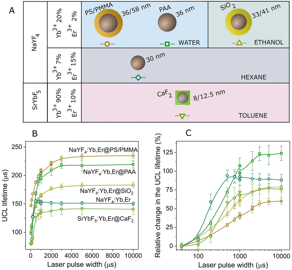 | ||
| Fig. 4 (A) Diagram illustrating the UCNPs under investigation, encompassing variations in host matrix, doping ratio, surface coating, size and solvent. (B) UCL lifetime as a function of the excitation pulse width, measured for the different types of UCNPs: (circles) water dispersion of NaYF4:Yb0.2,Er0.02@PS/PMMA, (squares) water dispersion of NaYF4:Yb0.2,Er0.02@PAA, (up-pointing triangles) ethanol dispersion of NaYF4:Yb0.2,Er0.02@SiO2, (diamonds) hexane dispersion of NaYF4:Yb0.07,Er0.15, and (down-pointing triangles) toluene dispersion of SrYb0.9F5:Er0.1@CaF2. (C) The UCL lifetime change versus the pulse width is presented relative to the value obtained at the shortest pulse width, utilizing the data from graph (B). All samples were measured using a laser power of 2.2 W. | ||
For example, UCNPs coated with polyacrylic acid (PAA), named NaYF4:Yb,Er@PAA, exhibit the most significant relative change in the UCL lifetime. While these nanoparticles share the same characteristics as those used in previous sections (NaYF4:Yb,Er@PS/PMMA), it has been proven that PAA provides less protection against surface quenching effects from water.30 Consequently, this results in a faster UCL decay (see Fig. 4B), particularly noticeable for short excitation pulses (∼100 μs for NaYF4:Yb,Er@PAA versus 150 μs for NaYF4:Yb,Er@PS/PMMA). As the excitation pulse width increases, other physical processes involving active ions less affected by surface quenching become more prominent, leading to a UCL lifetime comparable to that observed in NaYF4:Yb,Er@PS/PMMA. Essentially, NaYF4:Yb,Er@PAA nanoparticles exhibit a more pronounced variation in the UCL lifetime compared to NaYF4:Yb,Er@PS/PMMA. This observation aligns with findings by Gao et al., who demonstrated a reduction in lifetime change with pulse width by encapsulating the nanoparticles within an inert shell.25 These results were qualitatively elucidated by the coexistence of Er3+ ions with multiple decay times, with their contribution to lifetime differing depending on their spatial distribution within the nanoparticle.
Furthermore, in Fig. 4B and C, we observe a more rapid increase in the UCL lifetime for the UCNPs doped with 7% of Yb3+ ions and 15% of Er3+ ions (diamonds), compared with the traditional doping of 20% Yb3+ ions and 2% Er3+ ions. As previously reported,43the pathway for populating the green emission level involves energy transfer between Er3+ ions due to the higher concentration of Er3+ ions. This suggests that these UCNPs exhibit a distinct mechanism for UCL generation, potentially resulting in a different rate of increase.
We strongly believe that these results are not exclusive to Yb3+ and Er3+-codoped UCNPs but common to other rare-earth-doped UCNP systems. This reveals a spectrum of possibilities for further investigation.
3.3 Implications on FRET
Finally, we theoretically discuss one potential consequence of the pulse-width-dependent UCL lifetime. As we mentioned in the Introduction, UCNPs are attractive candidates as donors for FRET-based detection, which is currently a major research topic in the field of UCNPs. In fact, challenging questions, such as optimal UCNP sizes and structures, donor–acceptor distances, and UCNP coating and functionalization strategies that are optimal for improved FRET efficiencies,31,44–47 as well as the development of theoretical models to investigate this process in depth,26,28 have been the focus of recent studies. In a very interesting work, Bhuckory et al. demonstrated that the UCL decay dynamics of 24 nm NaYF4:Yb3+,Er3+ nanoparticles in a UCNPs–dye FRET system do not significantly change, whereas the UCL intensity shows a strong distance dependence to the dye.27 This suggests that UCL lifetimes may not be very suitable for analyzing FRET efficiencies. Recently, a dependence of the sensitivity of a FRET-based UCL sensor with the excitation pulse width has been reported.29 FRET is typically detected by measuring the change in the UCL lifetime attributed to the presence of the acceptor, which introduces a new nonradiative relaxation pathway. Then, FRET efficiency is commonly assessed using the following expression: | (2) |
 | (3) |
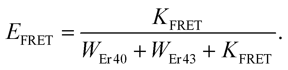 | (4) |
 | ||
| Fig. 5 (A) Schematic representation of the donor-UCNP–acceptor system used in the simulation. The decay rates for the green emission level are indicated: the radiative decay rate WEr40, the nonradiative decay rate to the next lower level WEr43, and the resonant energy transfer rate to the acceptor KFRET. (B) (left axis) Simulated UCL lifetime in the absence (black dashed line) and in the presence (black solid line) of an acceptor with a FRET efficiency of EFRET = 0.25. The laser intensity is I = 0.025Isat. (right axis) Using these curves we plotted the simulated FRET efficiency as a function of the laser pulse width (pink solid line). (C) A 2D contour plot of the simulated FRET efficiency, calculated based on the UCL lifetime change, as a function of the laser pulse width and laser intensity. | ||
We finally explored FRET under steady-state conditions, employing CW laser excitation. This method is generally not optimal for experimentally detecting FRET, mainly because luminescence reabsorption cannot be reliably distinguished from energy transfer. Moreover, luminescence is significantly influenced by variations in the concentration of UCNPs and the excitation irradiance. In this scenario, the FRET efficiency is determined by observing changes in the intensity of the UCL spectrum:
 | (5) |
3.4 Red and blue emission bands
We investigated the effect of the excitation pulse width on the UCL lifetime for the remaining visible emission bands of the Er3+/Yb3+-doped UCNPs. The UCL spectrum of the NaYF4:Yb0.2,Er0.02@PS/PMMA nanoparticles is plotted in Fig. 6A and consists of green (4S3/2 and 2H11/2 → 4I15/2), red (4F9/2 → 4I15/2), and blue (2H9/2 → 4I15/2) emission bands. Fig. 6B shows the energy-level scheme with these transitions. The power law relationship between the UCL intensity and the excitation intensity for the various emission bands highlights the nature of the underlying upconversion mechanism (see Fig. 6C). The green and red emissions follow a biphotonic process, i.e., a power law exponent close to 2, whereas the blue emission show a triphotonic process, i.e., a power law exponent close to 3. | ||
| Fig. 6 (A) UCL spectrum of the NaYF4:Yb0.2,Er0.02@PS/PMMA nanoparticles which includes emissions at 412 nm (blue) corresponding to the 2H9/2 → 4I15/2 transition, 520/540 nm (green) corresponding to the 2H11/2 and 4S3/2 → 4I15/2 transitions, and 655 nm (red) corresponding to the 4F9/2 → 4I15/2 transition. The spectrum of the laser used for excitation at 967 nm is also depicted in gray. (B) An energy-level diagram summarizes the three upconversion emissions and the laser absorption. (C) UCL intensity for the green, red, and blue emissions plotted as a function of the excitation laser intensity for the NaYF4:Yb0.2,Er0.02@PS/PMMA nanoparticles. Symbols represent measurements, and solid lines indicate linear fits to the data. (D) UCL lifetime versus laser pulse width for the red and blue emission bands at a laser power of 2.2 W measured for the different UCNPs: (circles) water dispersion of NaYF4:Yb0.2,Er0.02@PS/PMMA, (squares) water dispersion of NaYF4:Yb0.2,Er0.02@PAA, (up-pointing triangles) ethanol dispersion of NaYF4:Yb0.2,Er0.02@SiO2, and (diamonds) hexane dispersion of NaYF4:Yb0.07,Er0.15. (E) Relative change in UCL lifetime, normalized with the value at the shortest pulse duration, versus laser pulse width for the data presented in graph (D). | ||
Fig. 6D shows the UCL lifetime as a function of the laser pulse width for both the red and blue emission bands across various types of UCNPs while maintaining a constant laser power of 2.2 W. While the behavior of the blue emission for the different UCNPs resembles that of the green emission, the red emission does not exhibit a similar pattern. To observe this dependence more clearly, we plotted in Fig. 6E the relative change in lifetime, normalizing it with the value at the smallest pulse width. The change in the UCL lifetime for the blue emission spans from 40% to 90% for the different UCNPs, which is comparable (though slightly smaller) to the range observed for the green emission (see Fig. 4C). This suggests the possibility that the blue emitting level is populated via energy transfer from the green emitting level (4S3/2). However, the red emission of all the nanoparticles studied shows only minimal variation with the laser pulse width, less than 10%, in agreement with previous findings reported by Han et al.22 This indicates that not all emissions behave similarly. One plausible explanation is that the population of the red level is not exclusively derived from the green level; otherwise, we would expect a similar trend of lifetime with pulse width. Alternative excitation pathways, possibly originating from the metastable level of Er3+ ions (4I13/2), may contribute to the population of the red level. This competition among mechanisms could potentially lead to unchanged decay dynamics despite a varying pulse duration.
4 Conclusions
We have investigated the impact of the excitation pulse duration on the temporal dynamics of the green upconversion luminescence in NaYF4:Yb0.2,Er0.02 nanoparticles. As a general trend, we observed an increase in the UCL lifetime when the laser pulse width extends from the microsecond to the millisecond range, eventually reaching saturation. This phenomenon was also observed in other UCNPs with varying sizes, coatings, doping concentrations of rare-earth ions, host matrices, and solvents. Notably, enhancements in the UCL lifetime exceeding 100% were achieved. The relationship among laser pulse width, laser power, and beam size in influencing the behavior of the UCL lifetime was investigated. We concluded that the laser fluence governs the UCL decay dynamics, as this parameter determines how the various energy levels of the Er3+ and Yb3+ ions are populated at the end of the laser pulse.The variation in UCL lifetime with the excitation pulse width was theoretically explained through a rate equation analysis. This allowed us to confirm the history-dependent nature of the UCL lifetime. In other words, the decay dynamics of UCL depends on the populations of the different energy levels of rare-earth ions reached at the end of the excitation pulse. Using the theoretical model, we demonstrated that the FRET efficiency, assessed by changes in the UCL lifetime, exhibits a dependence on the laser pulse width. Therefore, great care must be taken when comparing the efficiencies of UC-based FRET sensors obtained under different experimental excitation conditions. Furthermore, we concluded that quantifying FRET in this kind of system presents a challenge that merits additional thoughtful consideration.
We have examined the impact of excitation pulse width on the red and blue UCL lifetimes using different types of UCNPs. While the blue emission behaves similarly to the green emission, the red emission shows minimal variation with the laser pulse width.
Our findings raise compelling questions that demand a more detailed investigation. For example, the behavior of the downshifting luminescence lifetime with excitation parameters needs to be explored, not only in rare-earth-doped nanoparticles but also in other luminescent nanosystems, such as quantum dots. On the other hand, this phenomenon opens up new possibilities for potential applications that leverage the relationship between lifetime and excitation power.
Conflicts of interest
There are no conflicts to declare.Acknowledgements
This work was supported by Ministerio de Ciencia e Innovación (PID2021-122806OB-I00, PID2021-123318OB-I00, TED2021-132317B-I00), Fundación Familia Alonso (2024/0041), and Comunidad de Madrid (P2022/BMD-7403 RENIM-CM). A. C. R. thanks UCM-Santander for a predoctoral contract (CT15/23).References
- F. Auzel, Chem. Rev., 2004, 104, 139–174 CrossRef CAS PubMed.
- D. K. Chatterjee, A. J. Rufaihah and Y. Zhang, Biomaterials, 2008, 29, 937–943 CrossRef CAS PubMed.
- E. M. Mettenbrink, W. Yang and S. Wilhelm, Adv. Photonics Res., 2022, 3, 2200098 CrossRef CAS PubMed.
- N. Sirkka, A. Lyytikäinen, T. Savukoski and T. Soukka, Anal. Chim. Acta, 2016, 925, 82–87 CrossRef CAS PubMed.
- D. Mendez-Gonzalez, M. Laurenti, A. Latorre, A. Somoza, A. Vazquez, A. I. Negredo, E. López-Cabarcos, O. G. Calderón, S. Melle and J. Rubio-Retama, ACS Appl. Mater. Interfaces, 2017, 9, 12272–12281 CrossRef CAS.
- M. S. Arai and A. S. S. de Camargo, Nanoscale Adv., 2021, 3, 5135–5165 RSC.
- G. Chen, H. Qiu, P. N. Prasad and X. Chen, Chem. Rev., 2014, 114, 5161–5214 CrossRef CAS PubMed.
- M. You, J. Zhong, Y. Hong, Z. Duan, M. Lin and F. Xu, Nanoscale, 2015, 7, 4423–4431 RSC.
- M. Schoenauer Sebag, Z. Hu, K. de Oliveira Lima, H. Xiang, P. Gredin, M. Mortier, L. Billot, L. Aigouy and Z. Chen, ACS Appl. Energy Mater., 2018, 1, 3537–3543 CrossRef CAS.
- N. Yadav and A. Khare, in Applications of Upconversion Nanoparticles for Solar Cells, ed. V. Kumar, I. Ayoub, H. C. Swart and R. Sehgal, Springer Nature Singapore, Singapore, 2023, pp. 339–367 Search PubMed.
- P. Alonso-Cristobal, O. Oton-Fernandez, D. Mendez-Gonzalez, J. F. Díaz, E. Lopez-Cabarcos, I. Barasoain and J. Rubio-Retama, ACS Appl. Mater. Interfaces, 2015, 7, 14992–14999 CrossRef CAS PubMed.
- D. Jaque and F. Vetrone, Nanoscale, 2012, 4, 4301–4326 RSC.
- J. C. Martins, A. Skripka, C. D. S. Brites, A. Benayas, R. A. S. Ferreira, F. Vetrone and L. D. Carlos, Front. Photon., 2022, 3, 1037473 CrossRef.
- M. E. Raab, S. L. Maurizio, J. A. Capobianco and P. N. Prasad, J. Phys. Chem. B, 2021, 125, 13132–13136 CrossRef CAS.
- J. Suyver, J. Grimm, M. van Veen, D. Biner, K. Krämer and H. Güdel, J. Lumin., 2006, 117, 1–12 CrossRef CAS.
- F. Wang and X. Liu, Chem. Soc. Rev., 2009, 38, 976–989 RSC.
- Y. Han, X. Zhang and L. Huang, Chem. – Eur. J., 2023, 29, e202302633 CrossRef CAS PubMed.
- Y. Chai, X. Zhou, X. Chen, C. Wen, J. Ke, W. Feng and F. Li, ACS Appl. Mater. Interfaces, 2022, 14, 14004–14011 CrossRef CAS PubMed.
- J. Bergstrand, Q. Liu, B. Huang, X. Peng, C. Würth, U. Resch-Genger, Q. Zhan, J. Widengren, H. Ågren and H. Liu, Nanoscale, 2019, 11, 4959–4969 RSC.
- T. A. Laurence, Y. Liu, M. Zhang, M. J. Owen, J. Han, L. Sun, C. Yan and G.-y. Liu, J. Phys. Chem. C, 2018, 122, 23780–23789 CrossRef CAS.
- D. R. Gamelin and H. U. Gudel, in Upconversion Processes in Transition Metal and Rare Earth Metal Systems, ed. H. Yersin, Springer Berlin Heidelberg, Berlin, Heidelberg, 2001, pp. 1–56 Search PubMed.
- Y. Han, C. Gao, T. Wei, K. Zhang, Z. Jiang, J. Zhou, M. Xu, L. Yin, F. Song and L. Huang, Angew. Chem., Int. Ed., 2022, 61, e202212089 CrossRef CAS PubMed.
- D. J. Gargas, E. M. Chan, A. D. Ostrowski, S. Aloni, M. V. P. Altoe, E. S. Barnard, B. Sanii, J. J. Urban, D. J. Milliron, B. E. Cohen and P. J. Schuck, Nat. Nanotechnol., 2014, 9, 300–305 CrossRef CAS.
- A. Teitelboim, B. Tian, D. J. Garfield, A. Fernandez-Bravo, A. C. Gotlin, P. J. Schuck, B. E. Cohen and E. M. Chan, J. Phys. Chem. C, 2019, 123, 2678–2689 CrossRef CAS.
- Y. Gao, J. Liu, J. Wan, M. Guo, M. Wei, K. Xu, Z. Yuan and X. Xie, J. Lumin., 2024, 266, 120325 CrossRef CAS.
- F. Pini, L. Francés-Soriano, N. Peruffo, A. Barbon, N. Hildebrandt and M. M. Natile, ACS Appl. Mater. Interfaces, 2022, 14, 11883–11894 CrossRef CAS PubMed.
- S. Bhuckory, S. Lahtinen, N. Höysniemi, J. Guo, X. Qiu, T. Soukka and N. Hildebrandt, Nano Lett., 2023, 23, 2253–2261 CrossRef CAS PubMed.
- F. Pini, L. Francés-Soriano, V. Andrigo, M. M. Natile and N. Hildebrandt, ACS Nano, 2023, 17, 4971–4984 CrossRef CAS PubMed.
- A. M. Kotulska, A. Pilch-Wróbel, S. Lahtinen, T. Soukka and A. Bednarkiewicz, Light: Sci. Appl., 2022, 11, 256 CrossRef CAS PubMed.
- D. Mendez-Gonzalez, V. Torres Vera, I. Zabala Gutierrez, C. Gerke, C. Cascales, J. Rubio-Retama, O. G. Calderón, S. Melle and M. Laurenti, Small, 2022, 18, 2105652 CrossRef CAS PubMed.
- S. Melle, O. G. Calderon, M. Laurenti, D. Mendez-Gonzalez, A. Egatz-Gómez, E. López-Cabarcos, E. Cabrera-Granado, E. Díaz and J. Rubio-Retama, J. Phys. Chem. C, 2018, 122, 18751–18758 CrossRef CAS.
- T. Stacewicz and M. Krainska-Miszczak, Meas. Sci. Technol., 1997, 8, 453–455 CrossRef.
- D. Mendez-Gonzalez, S. Melle, O. G. Calderón, M. Laurenti, E. Cabrera-Granado, A. Egatz-Gómez, E. López-Cabarcos, J. Rubio-Retama and E. Díaz, Nanoscale, 2019, 11, 13832–13844 RSC.
- M. A. de Araújo, R. Silva, E. de Lima, D. P. Pereira and P. C. de Oliveira, Appl. Opt., 2009, 48, 393–396 CrossRef PubMed.
- R. Arppe, I. Hyppänen, N. Perälä, R. Peltomaa, M. Kaiser, C. Würth, S. Christ, U. Resch-Genger, M. Schäferling and T. Soukka, Nanoscale, 2015, 7, 11746–11757 RSC.
- S. Lahtinen, A. Lyytikäinen, H. Päkkilä, E. Hömppi, N. Perälä, M. Lastusaari and T. Soukka, J. Phys. Chem. C, 2017, 121, 656–665 CrossRef CAS.
- O. Plohl, M. Kraft, J. Kovač, B. Belec, M. Ponikvar-Svet, C. Würth, D. Lisjak and U. Resch-Genger, Langmuir, 2017, 33, 553–560 CrossRef CAS PubMed.
- R. B. Anderson, S. J. Smith, P. S. May and M. T. Berry, J. Phys. Chem. Lett., 2014, 5, 36–42 CrossRef CAS PubMed.
- N. U. Wetter, A. M. Deana, I. M. Ranieri, L. Gomes and S. L. Baldochi, IEEE J. Quantum Electron., 2010, 46, 99–104 CAS.
- S. Fischer, H. Steinkemper, P. Löper, M. Hermle and J. C. Goldschmidt, J. Appl. Phys., 2012, 111, 013109 CrossRef.
- M. Kaiser, C. Würth, M. Kraft, T. Soukka and U. Resch-Genger, Nano Res., 2019, 12, 1871–1879 CrossRef CAS.
- J. Dormand and P. Prince, J. Comput. Appl. Math., 1980, 6, 19–26 CrossRef.
- V. Torres Vera, D. Mendez-Gonzalez, D. J. Ramos-Ramos, A. Igalla, M. Laurenti, R. Contreras-Caceres, E. Lopez-Cabarcos, E. Diaz, J. Rubio-Retama, S. Melle and O. G. Calderon, J. Mater. Chem. C, 2021, 9, 8902–8911 RSC.
- O. Dukhno, F. Przybilla, M. Collot, A. Klymchenko, V. Pivovarenko, M. Buchner, V. Muhr, T. Hirsch and Y. Mély, Nanoscale, 2017, 9, 11994–12004 RSC.
- A. Pilch-Wrobel, A. M. Kotulska, S. Lahtinen, T. Soukka and A. Bednarkiewicz, Small, 2022, 18, 2200464 CrossRef CAS PubMed.
- Y. Wang, K. Liu, X. Liu, K. Dohnalová, T. Gregorkiewicz, X. Kong, M. C. G. Aalders, W. J. Buma and H. Zhang, J. Phys. Chem. Lett., 2011, 2, 2083–2088 CrossRef CAS.
- L. Francés-Soriano, N. Estebanez, J. Pérez-Prieto and N. Hildebrandt, Adv. Funct. Mater., 2022, 32, 2201541 CrossRef.
Footnote |
| † Electronic supplementary information (ESI) available: High-resolution transmission electron microscopy (HR-TEM) characterization; excitation pulse widths and repetition frequencies; fitting the UCL decay curves; UCL lifetime at different temperatures; laser beam diameter measurement; parameter values used in the theoretical model; simulated UCL decay curves; UCNPs morphological characterization; FRET efficiency with steady-state luminescence. See DOI: https://doi.org/10.1039/d4nr00718b |
| This journal is © The Royal Society of Chemistry 2024 |