Synthesis and characterisation of neodymium-based MOFs for application in carbon dioxide reduction to syngas

Abstract

Two new neodymium-based metal–organic frameworks, JMS-10 and JMS-11, were synthesised using a 2,2′-bipypridine-5,5′-dicarboxylic acid (bpdc) linker. Both MOFs were solvothermally synthesised in DMF under different conditions. JMS-10 was synthesised at 120 °C while JMS-11 was synthesised at 100 °C in the presence of a modulator. Both the MOFs possessed very similar crystallographic parameters but were found to be structurally diverse. Their structures were built by secondary building units (SBUs) made up of carboxylates binding in sets of four and two to the straight rod, thus forming two types of alternating nodes that are 6- and 4-connected. Both JMS-10 and JMS-11 were functionalized using the ruthenium p-cymene complex. The functionalized MOFs were applied in the photocatalytic reduction of carbon dioxide to syngas where they produced both hydrogen and carbon monoxide (CO : H₂) in the ratio of 1 : 2. The amount of CO to H₂ produced varied depending on the additives used in the reaction medium, highlighting the importance of water, triethanolamine and acetonitrile in tuning the syngas ratio for different industrial applications.

---

Introduction

The rise of the industrial revolution had both positive and negative effects on the world at large. Inasmuch as people enjoyed the increased production of goods, efficiency, lower prices of goods, improved wages and development of areas, the industrial revolution contributed immensely to the levels of pollution in the environment, especially in global warming. The chief culprit of this challenge happens to be carbon dioxide, which is a product of the burning of fossil fuels in the production of energy in factories and vehicles.¹ Efforts are being made to reduce the CO₂ concentrations in the atmosphere using clean fuels such as methanol, ethane and methane as alternatives to fossil fuels.² The use of sunlight is also another efficient method because it is an unlimited and clean source of energy. Other viable methods are being developed whereby carbon dioxide is stored underground³ or converted to other useful chemicals.⁴

The C⁴⁺ atom in CO₂ is in its fully oxidized state, making CO₂ highly thermodynamically stable; this presents a challenge in its direct conversion.^3–5 To overcome this challenge, a catalyst is required to make the process easier. Chemical catalysts such as those of platinum group metals have proven to be highly active in many processes including carbon dioxide reduction. To enhance their catalytic properties, these catalysts can be supported in various materials including metal–organic frameworks (MOFs).^6,7 MOFs have become an outstanding group of porous materials in reticular chemistry.^8,9 These materials present unique properties, including high surface areas,¹⁰ tunable porosity, structural rigidity and diversity,¹¹ flexible network topology and chemical functionality.¹² These properties can be accredited to the periodic structures formed when the organic linkers and the inorganic metal ions are combined.^13,14 The backbone of MOFs that has gained so much attention is the secondary building unit (SBU). SBUs can be simplified as geometric figures comprising metal clusters connected through non-metal bonds, typically organic components such as the oxo (M–O–M) and carboxylate (M–O–C–O–M) form recurrent 3D structures.^13,15 The catalytic activity coupled with the stability of MOFs makes them superior materials, especially in photocatalysis, where they can be functionalized with other catalysts to enhance their photocatalytic properties.

Numerous studies have been conducted that focus on the artificial reduction of carbon dioxide, and these include thermocatalytic,^4,16 biocatalytic,^17,18 electrochemical,^19,20 bioelectrocatalytic^21,22 and photocatalytic methods.^3,5,23–27 Electrochemical and thermocatalytic methods require extra energy to be input into the process, which becomes costly. Biocatalytic and bioelectrocatalytic methods also require ambient conditions for biological molecules not to denature, which is very difficult to maintain for good product yields. This makes photocatalytic reduction a better method due to its energy efficiency and environmental friendliness because it uses free and clean solar energy, which is also abundant.³ Photocatalytic conversion of CO₂ into various industrially important products, such as methanol, methane, carbon monoxide and ethane, has been widely studied.^28–30 The first photocatalytic reduction of CO₂ was reported in 1979 in aqueous suspensions of semiconductors, such as ZnO, TiO₂, GaP, SiC and CdS, to produce formaldehyde, formic acid and methanol.³¹ Since then, many studies have been reported on photocatalytic reduction of CO₂ to various products and titanium dioxide, and its modified counterparts have been widely explored as photocatalysts.^32–37 Photocatalytic reduction of CO₂ can be done either in liquid or gas phase. In the liquid phase, the photocatalyst is usually mixed with sacrificial electron donors and other supporting reagents that are also in the liquid phase. Then, CO₂ is bubbled through the solution, after which the mixture is irradiated with solar light for some time, and the products are collected and analysed usually with gas chromatography (GC). In the gas phase, however, a minimum amount or no liquid reagents are used, and the products are usually in the gas phase.

CO₂ reduction to syngas has recently gained popularity because syngas is an important feedstock in many industrial processes, such as methanol production,³⁸ hydroformylation and the Fischer–Tropsch synthesis.^39,40 The ratios of the CO to H₂ gases in the syngas are important for the various productions; for example, methanol production requires a CO/H₂ ratio of 1 : 2, whereas hydroformylation requires 1 : 1 and Fischer–Tropsch synthesis requires 1 : 2 or 2 : 1.⁴⁰ In this work, two new rod MOFs (JMS-10 and JMS-11) were synthesised from the neodymium metal salt and 2,2′-bipyridine-5,5′-dicarboxylic acid linker in dimethylformamide under different conditions. The high coordination number associated with neodymium metal gives rise to chemical and thermal stability in MOFs, making them highly suitable as support materials for molecular catalysts.

The MOFs were functionalised with the ruthenium p-cymene complex and then used for the photocatalytic reduction of CO₂ to syngas. The functionalised MOFs showed activity towards the reduction of CO₂ to syngas.

Experimental

Materials and chemicals

Neodymium nitrate (NdNO₃·6H₂O) was purchased from Sigma-Aldrich, and 2,2-bipyridine-5,5′-dicarboxylic acid was purchased from Thermo Scientific. Acetic acid glacial was obtained from Fisher Chemicals. 1,10-Phenanthroline and dimethyl formamide (DMF) were also purchased from Sigma-Aldrich, Germany.

Synthesis of JMS-10 [Nd₂O(bpdc)₃(H₂O)₂·3DMF]

JMS-10 was synthesised from neodymium nitrate hexahydrate and 2,2′-bipyridine-5,5′-dicarboxylic acid linker (Scheme S1, ESI†). 0.375 mmol (0.1644 g) of neodymium nitrate hexahydrate and 0.1875 mmol of 2,2-bipyridine-5,5′-dicarboxylic acid were dissolved in 4 mL DMF, sealed in an autoclave and heated at 120 °C. After 6 hours of reaction, purple, star-like crystals were obtained.

Synthesis of JMS-11 [Nd₂O(bpdc)₃(DMF)₂·2DMF]

JMS-11 was prepared by mixing 0.2 mmol of neodymium nitrate hexahydrate, 0.1 mmol of 2,2′-bipyridine-5,5′-dicarboxylic acid, 3 mg of 1,10-phenanthroline and one drop of acetic acid (Scheme S2, ESI†). The reaction contents were dissolved in 10 mL of DMF and charged into an autoclave. The autoclave was placed in an oven that was pre-set at 100 °C. Single crystals were obtained after 72 hours.

Functionalisation of JMS-10 and JMS-11 with ruthenium

Ruthenium p-cymene (10 mg) was dissolved in 2 mL acetone in a small vessel. Then, 100 mg of the activated MOF was added to the solution. This was sonicated for 30 minutes and then left in a large vessel containing a small amount of diethyl ether for 24 hours. The small vessel was then removed, liquid decanted and MOF dried at 80 °C.

Single-crystal data collection

Single-crystal XRD data of JMS-10 were collected at 173 K using a Bruker KAPPA APEX II DUO diffractometer equipped with graphite-monochromated Mo Kα radiation (λ = 0.71073 Å). A total of 2322 frames were collected. The total exposure time was 16.12 hours. The frames were integrated with the Bruker SAINT⁴¹ software package using a narrow-frame algorithm. The integration of the data using a monoclinic unit cell yielded a total of 241812 reflections to a maximum θ angle of 30.50° (0.70 Å resolution). Data were corrected for absorption effects using the multi-scan method (SADABS). The ratio of minimum to maximum apparent transmission was 0.863. Unit-cell refinement and data reduction were performed using the program SAINT.⁴¹ The structures were solved by applying direct methods (program SHELXT⁴²) and refined anisotropically on F2 full-matrix least-squares using SHELXL⁴² within the X-SEED^43a interface. Anisotropic thermal parameters were applied to non-hydrogen atoms, while all hydrogen atoms were added at idealised positions. SADI and EADP restraints were used to obtain reasonable displacement coefficients. In JMS-10, SQUEEZE estimated approximately three disordered DMF.

A clear light, colourless block-shaped crystal of JMS-11 with dimensions 0.196 × 0.084 × 0.029 mm³ was mounted on a suitable support. Data were collected using an XtaLAB Synergy R HyPix diffractometer operating at T = 143.8(3) K. Data were measured using ω scans of 0.5° per frame for 0.5/2.1 s with Cu Kα radiation. The diffraction pattern was indexed, and the total number of runs and images was based on the strategy calculation from the program CrysAlis^Pro. The maximum resolution achieved was Θ = 75.7° (0.79 Å). Data reduction and scaling were achieved using the CrysAlis^Pro software package (CrysAlis^Pro 1.171.42.49).^43b A numerical absorption correction using a numerical grid with Gaussian integration for the multifaceted crystal model faces was applied. Empirical absorption correction was performed using spherical harmonics, as implemented in the SCALE3 ABSPACK scaling algorithm. The absorption coefficient μ of this material is 15.901 mm⁻¹ at this wavelength (λ = 1.542 Å). The structure was solved and the space group P2₁/c (# 14) was determined by the ShelXT structure solution program using Intrinsic Phasing and refined by Least Squares using version 2016/6 of ShelXL 2016.⁴² All non-hydrogen atoms were refined anisotropically. Hydrogen atom positions were calculated geometrically and refined using the riding model. The structures were deposited in the Cambridge Database with deposition numbers CCDC 2249596 and CCDC 2249598. Table S1 (ESI†) lists the crystallographic and refinement parameters of the two MOFs.

Powder X-ray diffraction

Powder X-ray diffraction (PXRD) data were collected using a BRUKER D2 Phaser diffractometer (Cu Kα radiation) equipped with a LYNXEYE XE-T detector. X-rays were generated with a current flow of 10 mA and a voltage of 30 kV. Variable temperature PXRD data were collected using the Panalytical X'Pert Pro (Cu Kα1 and Kα2 radiation) equipped with an X Celerator detector. X-rays were generated with a current flow of 40 mA and a voltage of 40 kV.

Thermal analysis

Thermogravimetric analysis (TGA) was performed using a TA Discovery Instrument TA-Q50 at a heating rate of 10 °C min⁻¹ with a temperature range of 25–500 °C under a dry nitrogen purge gas flow of 50 mL min⁻¹.

Fourier transform infrared (FTIR) studies

FTIR spectra of the samples were recorded in the range of 400–4000 cm⁻¹ using a Perkin-Elmer FTIR spectrophotometer (Model BX II) fitted with an attenuated total reflectance (ATR) probe.

Scanning electron microscopy (SEM)

SEM images of the activated JMS-10 and JMS-11 MOFs were collected using a TESCAN MIRA3 FEG-SEM. The voltage was 5.0 kV, and the magnifications of 100 μm, 150 μm and 500 μm were used.

Transmission electron microscopy (TEM)

The Talos F200X G2 is a 200 kV FEG scanning transmission electron microscope (S/TEM) that was used to collect TEM images of the samples. The instrument is equipped with a Schottky X-FEG electron source operated at accelerating voltages of 60, 80, 120 or 200 kV. It also has a Ceta 16M camera with speed enhancement designed for imaging and diffraction applications. It allows 4k × 4k images to be acquired at 40 frames per second (and 512 × 512 pixels at 320 fps). HAADF, DF2, DF4 and BF STEM detectors are used in this instrument.

Nuclear magnetic resonance (NMR)

A Bruker Avance III 500 MHz DCH Cryoprobe Spectrometer was used for the NMR analysis of the samples. The instrument was able to observe ¹H nuclei. The results were analysed using the Bruker TOPSPIN 3.0 software.

Photocatalysis process

The functionalized MOFs (5 mg) were placed in 7.74 mL vials. 3 mL of a solvent containing 0.1 M triethanolamine (TEOA) in a 1 : 1 v/v mixture of acetonitrile:water was added, followed by sonication for 30 min. The vials were capped with rubber seums and purged with CO₂ containing 2% CH₄ gas for 15 min. The vials were then placed in a photocatalysis reactor under the following conditions: 100 mW cm⁻² (1 sun, AM 1.5G) at 25 °C, with stirring. The reaction mixture was irradiated for 22 hours. The gaseous products produced were analysed using gas chromatography.

Gas chromatography (GC)

The gaseous H₂ and CO produced were analyzed by a Shimadzu GC-2010 Plus gas chromatograph equipped with a Hayesep D precolumn, an RT molecular sieve 5 A column and a thermal conductivity detector using He as the carrier gas. Methane (2% in N₂ gas) was used as an internal standard. 50 μL of headspace gas from the photoreactor was injected using an air-tight Hamilton syringe, and the amounts of the gases were detected and recorded.

Results and discussion

Structural description

JMS-10 and JMS-11 had very close crystallographic parameters, as shown in Table S1 (ESI†). Both MOFs were crystallized in a monoclinic crystal system and P2₁/c space group. In JMS-10, two crystallographically independent Nd³⁺ centres, three pbdc linkers, and two coordinated water molecules were modelled in their asymmetric unit. Several disordered solvent molecules were observed in the asymmetric unit. SQEEZE in Platon⁴⁴ estimated approximately three DMF molecules. The two Nd(III) metal centres exhibited similar coordination environments, with both centres coordinated to six oxygen atoms of the linker and two water molecules to furnish a square antiprismatic geometry, as shown in Fig. 1.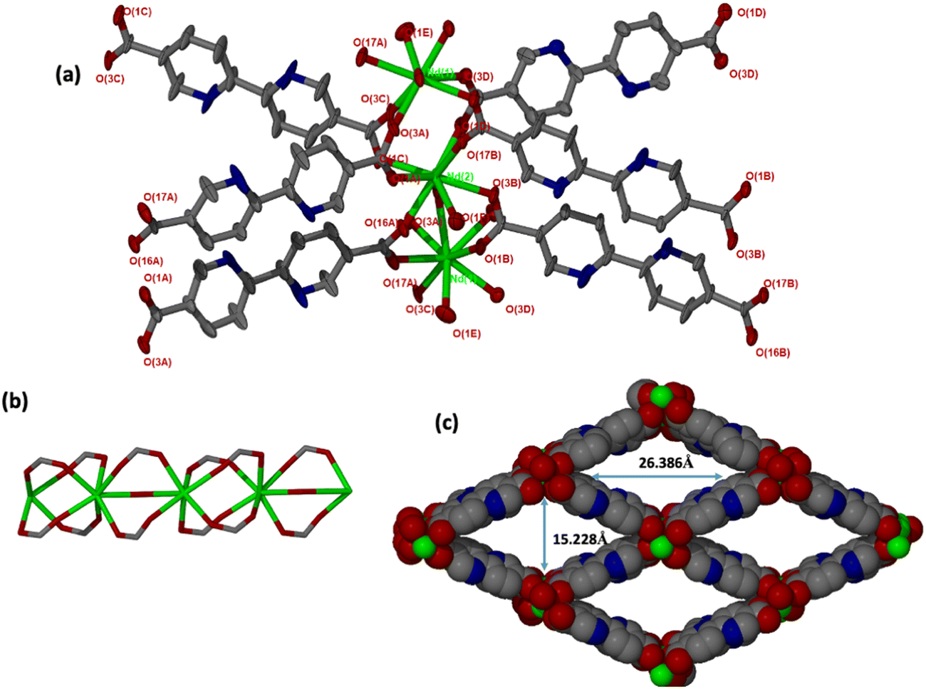

Fig. 1 (a) Coordination environment in JMS-10 showing the linkers surrounding the metal centres. Hydrogens were omitted for clarity. (b) Rod SBU found in JMS-10, and (c) packing diagram of JMS-10 showing channel dimensions as viewed along the c-axis.

In JMS-11, two metal centres, three pbdc linkers, two coordinated DMF molecules and one bridging oxygen atom were modelled. A further two uncoordinated DMF molecules were also modelled. The coordination environments of the two metal centres (Nd1 and Nd2) are similar. Both metals are coordinated to six oxygen atoms from the linkers: one oxygen atom of the DMF molecule and a bridging oxygen atom to furnish a square antiprismatic geometry.

JMS-11 had a smaller unit cell volume compared to JMS-10 (Table S1, ESI†). The smaller unit cell volume originates from the bending nature of the pbdc linkers, which buckle inside the channels. This effectively reduces the distance between the rod SBUs. The structure of JMS-10 is made up of Nd₂C₄O₈ and Nd₂C₂O₅ secondary building unit (SBU) rods that grow along the c-axis (Fig. 1b). Interestingly, these two SBUs are found in the rod alternates in an ABAB fashion. The structure of JMS-11 is also built by a rod similar to JMS-10, which consists of two alternating SBU units of Nd₂C₄O₈ and Nd₂C₂O₅ (Fig. 2b). The bpdc linkers connect the rods to give 3D structures with large rhombic channels of 26.386 Å by 15.228 Å (Fig. 1c) in JMS-10. However, JMS-11 exhibits small pores in the absence of solvated DMF molecules (Fig. 2c). The solvent accessible surface was modelled using the Mercury program using a probe radius of 1.2 Å and grid spacing of 0.7 Å.⁴⁵ JMS-10 has a solvent-accessible void volume of 27%. However, JMS-11 had a lower solvent accessible void volume of 3% attributed to the presence of coordinated DMF molecules. The 2,2′-bipyridine-5,5′-dicarboxylate linker used in the synthesis of the two MOFs showed a great deal of flexibility, as evidenced by the torsional angles formed within the linkers of the frameworks, especially in JMS-10 (Fig. 3a). These torsional angles aided in creating larger and more open channels in the MOF. Three of the linkers in JMS-10 had torsional angles of 166.33(7)° to approximately 168.9(11)°, and the other had a torsional angle of 180.00(4)°. However, JMS-11 had linkers with torsional angles close to 180°, with one linker having a torsional angle of 172.7(7)° (Fig. 3b). In JMS-10, the flexibility observed between the phenyl rings of the linker gave rise to open channels. On the contrary, the buckling in and out of the linkers in JMS-11 may have restricted the rotation between the phenyl rings, reducing the distance between adjacent SBU and giving rise to smaller channels.

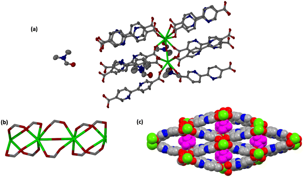Fig. 2 (a) Coordination environment in JMS-11 showing the linkers surrounding the metal centres. Hydrogens are omitted for clarity, and coordinated and uncoordinated DMF molecules are also shown. (b) Rod SBU and (c) packing diagram of JMS-11 viewed along the c-axis; the guest coordinated DMF molecules are shown in purple.

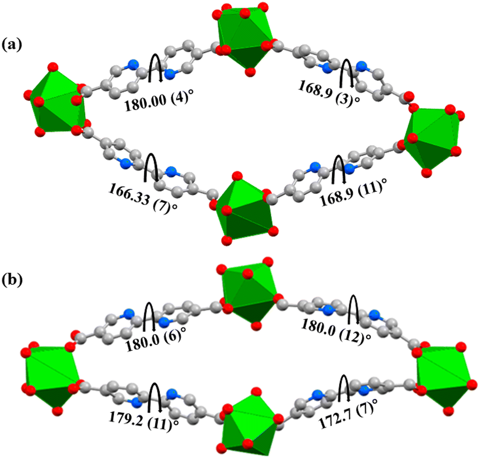Fig. 3 Linker flexibility in (a) JMS-10 channel and (b) JMS-11 channel. Diagrams showing the torsional (dihedral) angles within the linkers.

The unit cell parameters of JMS-10 and JMS-11 were too close. Their calculated PXRD patterns were compared to rule out the possibility of these structures being isostructural. As illustrated in Fig. S1 (ESI†), it can be confirmed that the two MOFs are not isostructural because their PXRD patterns are different. JMS-10 and JMS-11 are highly crystalline, showing good agreement between the calculated PXRD and the as-synthesised MOFs, as shown in Fig. 4a and b for JMS-10 and JMS-11, respectively. The major peaks on the experimental and calculated PXRD patterns correlated well for both MOFs, showing the phase purity of the synthesised MOFs.

Fig. 4 Simulated and experimental PXRD patterns (a) JMS-10 and (b) JMS-11; TGA of (c) JMS-10 and (d) JMS-11.

The thermal stability of JMS-10 and JMS-11 was studied using thermogravimetric analysis. Both MOFs were thermally stable, as shown by their TGA results. Both MOFs decompose above 425 °C (Fig. 4c and d). Thermal analysis of JMS-10 showed a 23.4% weight loss in the temperature range ranging from 50 °C to around 200 °C, as shown in Fig. 4c. This weight loss corresponds to the loss of three DMF molecules and two water molecules (calculated at 23.9%). The TGA thermogram of both the activated and native JMS-10 shows no significant weight loss between 340 °C and 425 °C, indicating high thermal stability after solvent loss until decomposition. JMS-11 showed a total weight loss of 25.3% within the same temperature range as JMS-10, as shown in Fig. 4d. Of special note was the 3% weight loss in JMS-11 in the temperature region of around 350 °C. This weight loss is also present in the activated material of the same MOF, which could be the onset of the decomposition of JMS-11 due to the loss of the carboxylate group. The literature has also proven that some MOFs with carboxylate linkers, such as MOF-5, tend to undergo decarboxylation, which releases CO₂ at 350 °C. MOF-5 was heated to 380 °C for 24 hours, and the TG-MS and VT-PXRD results showed a 60% loss of CO₂ units.⁴⁶ Variable temperature PXRD studies of the two MOFs are shown in Fig. S2 (ESI†). The two MOFs were thermally stable up to 400 °C. This result correlates well with the TGA results showing thermal degradation at around 425 °C for both MOFs. However, some peaks are lost as the temperature increases, especially at 100 °C for JMS-11, which could be attributed to the loss of coordinated and solvated water molecules. Interestingly, at 100 °C, the PXRD pattern for JMS-11 is the same as that of JMS-10. However, at 200 °C, JMS-11 loses the small peak at around 8.7 2θ degrees, which remains on JMS-10 until 500 °C, as shown in Figure S2 (ESI†). This means that JMS-11 changes its phase initially to JMS-10 at 100 °C and then again to another phase at higher temperatures. The PXRD of the sample collected at 500 °C exhibits the same diffraction pattern after cooling the sample to room temperature (25 °C). This suggests an irreversible structural transformation above 500 °C.

Chemical stability studies

PXRD studies were used to evaluate the stability of the two MOFs in several solvents (Fig. 5). Upon activation of both JMS-10 and JMS-11, major peaks at lower 2θ values were maintained, suggesting that the integrity of the MOFs was not affected by the removal of coordinated and uncoordinated solvent molecules residing in the channels. However, JMS-11 lost peaks at 8.5 and 17 2θ positions upon activation, as depicted in Fig. 5b. This is attributed to the loss of the coordinated water and DMF molecules, which has the effect of changing the geometry around the metal centre. However, upon soaking in water, the intense peak, which was lost upon activation, was observed at 8.5 2θ, suggesting that the water molecules could occupy the sites left by the coordinated guest molecules, which were removed upon activation. The rest of the solvents studied in both JMS-10 and JMS-11 had diffraction patterns similar to those of the activated material. This indicates that the solvents did not affect the MOF framework.

Fig. 5 PXRD stability results for (a) JMS-10 and (b) JMS-11 in various solvents.

The morphology of JMS-10 and JMS-11 was evaluated using SEM. As illustrated in Fig. 6 and 7, both MOFs had rod morphology; however, JMS-11 had rods aligned in the form of shrubs (forming multiple branches) (Fig. 7). JMS-10 had different particle sizes, which may be attributed to the different rates of crystallisation. JMS-11 had more uniform particle sizes that were well shaped, as shown in Fig. 7, a sign that the crystallisation rate in the synthesis of the crystals was also uniform. Another interesting observation was that JMS-10 had the most cracked crystals compared to JMS-11 (Fig. 6), with smooth, well-defined rod surfaces. This could be due to the higher synthesis temperature used in JMS-10. The SEM elementary mapping confirmed the presence and uniform distribution of the expected elements in the crystals, as shown in Fig. S3 and S4 (ESI†), for JMS-10 and JMS-11, respectively.

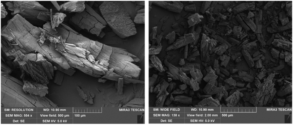Fig. 6 SEM images of JMS-10 at high magnification (left) and low magnification (right).

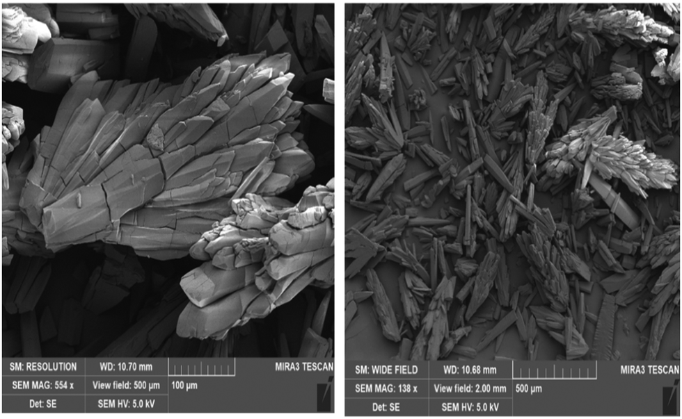Fig. 7 SEM images of JMS-11 at high magnification (left) and at low magnification (right).

Functionalisation of JMS-10 and JMS-11

JMS-10 and JMS-11 were functionalised using the ruthenium p-cymene complex, as described in the experimental section, to give Ru(II)@JMS-10 and Ru(II)JMS-11, respectively (Scheme S3, ESI†).

PXRD studies in Fig. 8 show similarities between the activated material and the ruthenium functionalised MOF. TEM studies on Ru(II)@JMS-10 and Ru(II)@JMS-11 indicated that the ruthenium particles were either dispersed on or close to the surface of the MOF crystals. Two areas were chosen on the TEM image, and EDX was performed on these specific areas to identify the ruthenium particles in the framework. Fig. 9a shows the TEM image of Ru(II)@JMS-10, and area marked 1 exhibits a significantly higher amount of ruthenium compared to area 2, as indicated by the peak intensity (Fig. 9b and c). Fig. 9d shows a section of the Ru(II)@JMS-11 rod composite. The image revealed whitish particles on the surface of the MOF (area marked 1) that contained more ruthenium than in area marked 2, as proven by EDX studies (Fig. 9e and f).

Fig. 8 PXRD of (a) JMS-10 and (b) JMS-11 and their corresponding derivatives.

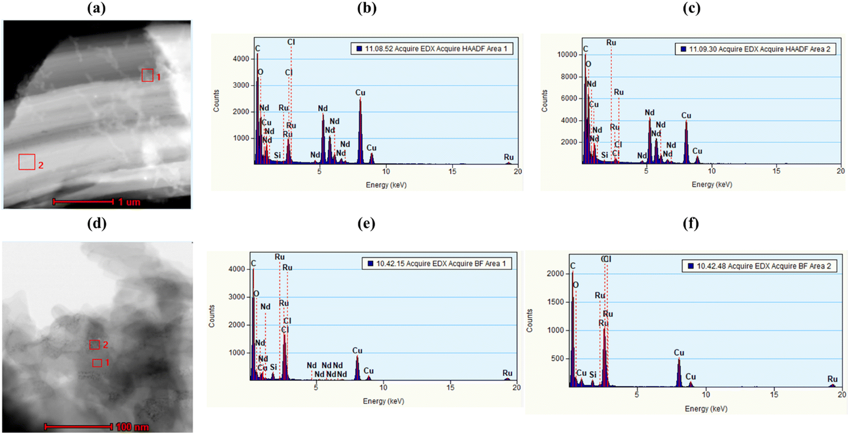Fig. 9 TEM and EDX images of Ru(II)@JMS-10 and Ru(II)@JMS-11 taken at 1 μm and 100 μm resolution, respectively. (a) TEM image for the Ru(II)@JMS-10 MOF showing area 1 with more Ru and area 2 with less Ru, (b) EDX for Ru(II)@JMS-10 area 1, (c) EDX for Ru(II)@JMS-10 area 2, (d) TEM image for the Ru functionalised JMS-11 MOF showing area 1 with more Ru and area 2, (e) EDX for Ru(II)@JMS-11 area 1 and (f) EDX for Ru(II)@JMS-11 area 2.

ICP-OES analysis of the functionalised MOFs showed an uptake of 2% and 1.8% of ruthenium by JMS-10 and JMS-11, respectively. Proton NMR was selectively done on JMS-10 and Ru(II)@JMS-10 MOF composites to check for the presence of the ruthenium p-cymene complex that was used for the functionalisation of the MOFs. As shown in Fig. S5 (ESI†), ¹H NMR proton signals at 6 ppm and 6.3 ppm, as well as between 1 ppm and 3 ppm, are attributed to the ruthenium p-cymene complex that was used in the functionalisation process. These peaks were unavailable on the JMS-10 ¹H NMR spectrum (Fig. S6, ESI†).

Further evidence of the presence of the functionalizing complex in the MOFs was provided by FTIR studies (Fig. 10). The band at 1642 cm⁻¹ in JMS-10 and its functionalized form can be attributed to the C–C vibrations of the pyridyl ring. The asymmetric and symmetric stretches of the carboxylate appear at 1564 cm⁻¹ and 1388 cm⁻¹, respectively, in both JMS-10 and Ru(II)@JMS-10. In JMS-11, the vibrations of the pyridyl ring are observed at 1671 and 1639 cm⁻¹ for the activated and functionalized forms, respectively. The positions of the asymmetric and symmetric carboxylate stretches moved to lower wave numbers after functionalisation. Of interest is the stretch at 2950 cm⁻¹ and 2968 cm⁻¹ in Ru(II)@JMS-10 and Ru(II)@JMS-11, respectively. This is due to the presence of the methyl group in the ruthenium p-cymene complex.

Fig. 10 FTIR studies of (a) JMS-10 and (b) JMS-11 and their corresponding derivatives.

The electronic states of the elements were also determined using XPS analysis. The XPS results for the ruthenium functionalised JMS-10 and JMS-11 MOF are presented in Fig. S7 and S8 (ESI†), respectively. The XPS survey spectra for the MOFs before and after functionalisation were compared to verify the presence of the catalysts. Fig. S7a and b (ESI†) show the XPS survey spectra for JMS-10 and Ru(II)@JMS-10, respectively. The functionalised MOFs show the presence of the ruthenium element, as evidenced by the doublet peaks centred at 464.7 eV and 494.8 eV for Ru 3p_3/2 and Ru 3p_1/2, respectively.⁴⁷ This proves that the oxidation state of the Ru in this case is +2, which again concurs with the oxidation state of ruthenium in the ruthenium p-cymene complex. XPS results of JMS-11 and its ruthenium functionalised derivative (Fig. S8, ESI†) are similar to those of JMS-10 with Ru(II)@JMS-11 showing the presence of the ruthenium.

Photocatalytic reduction of CO₂ to syngas (H₂ and CO)

Functionalised JMS-10 and JMS-11 were used for the photocatalytic reduction of CO₂ to syngas. The activated and functionalised MOF composites were soaked in a mixture of triethanolamine (TEOA), water and acetonitrile. CO₂ gas containing approximately 2% CH₄ was bubbled through the mixture for about 15 minutes. The mixture was then exposed to light in a solar simulator for 24 hours while stirring. The amount of H₂ and CO gas produced was measured using gas chromatography. Fig. 11a shows the amounts of the syngas produced using Ru@JMS-10, Ru@JMS-11, JMS-10, and JMS-11. The ruthenium functionalised MOFs showed activity towards syngas production as opposed to the unfunctionalised MOFs.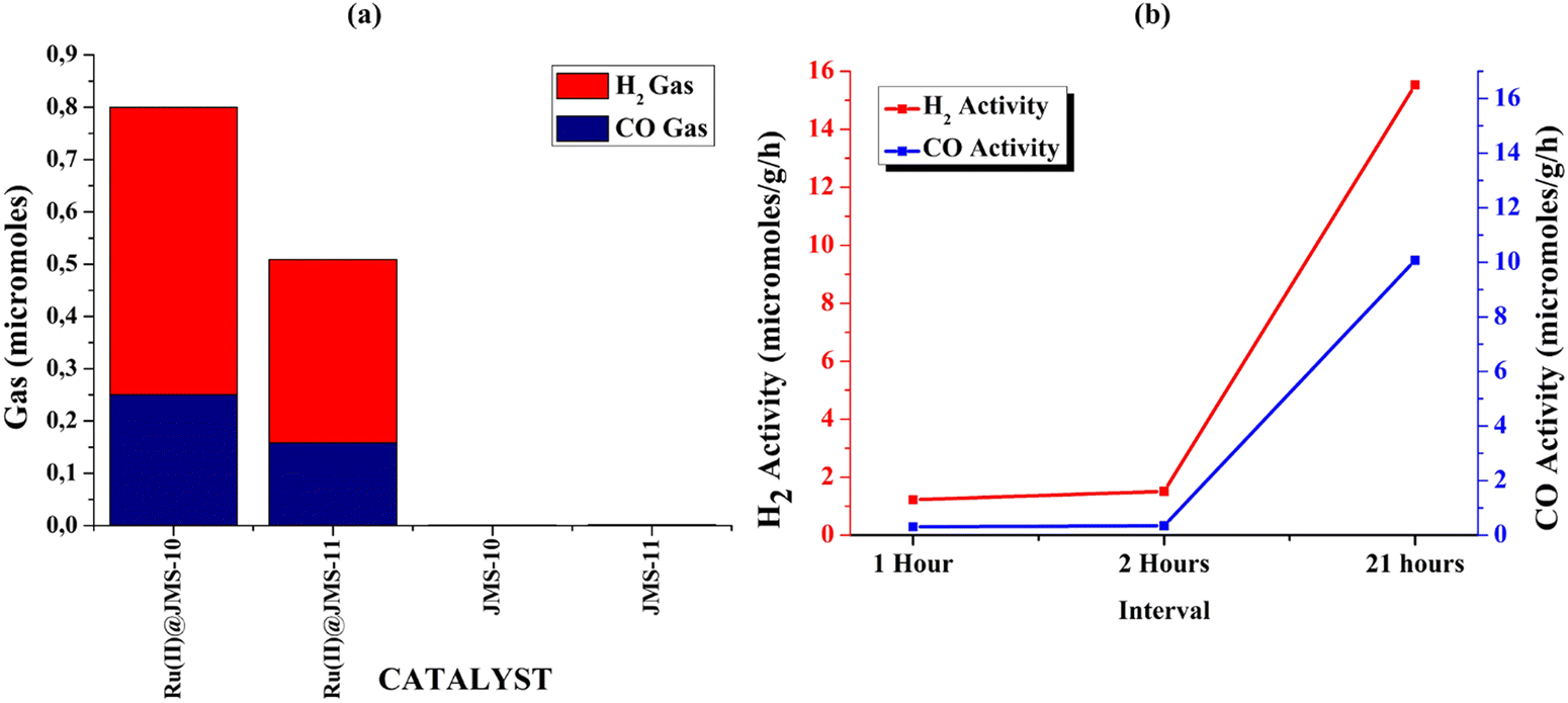

Fig. 11 Synthetic gas production from CO₂ using the functionalised JMS-10 and JMS-11. (a) The amount of syngas (CO and H₂) produced with Ru(II)@JMS-10, Ru(II)@JMS-11, JMS-10, and JMS-11; (b) kinetic experiments using Ru(II)@JMS-10 to monitor H₂ and CO production with time.

The effect of the additives on the production of syngas was evaluated using JMS-10 functionalised MOF (Table 1). Entry 1 shows that 6.33 × 10⁻¹ and 0.11 × 10¹ micromoles of H₂ and CO, respectively, were produced in the presence of TEOA/MeCN/H₂O using the Ru(II)@JMS-10 MOF. In the presence of the unfunctionalized JMS-10 MOF, insignificant amounts of the syngas were produced (entry 2). In the absence of water (entry 3), the amount of syngas produced by Ru(II)JMS-10 was reduced by approximately 800 times for H₂ and 373 times for CO. Furthermore, the ratio of CO to H₂ produced in the absence of water was approximately 1 : 1. With only water as an additive (entry 4), insignificant amounts of hydrogen were produced, highlighting the importance of TEOA/MeCN in the production of syngas. In the absence of TEOA (entry 5), the amount of syngas produced by Ru(II)@JMS-10 is also reduced with the ratio of CO to H₂ changing from 1 : 2 in entry 1 to approximately 2 : 1. The catalysis was successful with all three reagents (TEOA, acetonitrile, and H₂O) available, producing CO:H₂ gas in a ratio of 1 : 2. However, in the absence of TEOA (entry 5) and water (entry 3), the ratio of CO:H₂ changed to 2 : 1 and 1 : 1, respectively, with a significant decrease in the amount of syngas produced. This observation suggests that these additives are important for tuning the ratio of CO:H₂ for various industrial applications.

Table 1 Effect of additives on the production of syngas

Entry	Catalyst	Additives	H2 produced (micromoles)	CO produced (micromoles)	Approximate syngas ratio (CO/H2)
1	Ru(II)@JMS-10	TEOA/MeCN/H2O	5.5 × 10^−1	2.5 × 10^−1	1 : 2
2	JMS-10	TEOA/MeCN/H2O	2.00 × 10^−3	1.90 × 10^−4
3	Ru(II)@JMS-10	TEOA/MeCN	6.80 × 10^−3	6.70 × 10^−3	1 : 1
4	Ru(II)@JMS-10	H2O	8.00 × 10^−3	—
5	Ru(II)@JMS-10	MeCN/H2O	1.95 × 10^−3	3.50 × 10^−3	2 : 1

---

The importance of light was demonstrated by placing the samples in the dark for 24 hours. In this instance, no syngas was produced in both MOF composites. The kinetics of the syngas production was studied within the first 2 hours of production; then, the experiment was left to run for 21 hours. It was observed that in the first 2 hours, the syngas production was low but gradually increased to 10 μmol g⁻¹ h⁻¹ for H₂ and 16 μmol g⁻¹ h⁻¹ for the CO gas (Fig. 11b). This means that syngas production was not instant, and the process took time. Compared to other MOFs and polymeric compounds, functionalised JMS-10 and JMS-11 had commensurate activities, as shown in Table 2. This shows that these MOFs are potential catalysts for the reduction of CO₂ to syngas.

Table 2 Benchmark table comparing the functionalised MOFs to other composites used in syngas production

Catalyst	Photosensitizer	Sacrificial agent	H2 Produced	CO produced	Ref.
Ru(II)@JMS-10	RuPCy	TEOA	16.9 μmol g^−1 h^−1 (TON = 9)	14 μmol g^−1 h^−1 (TON = 3.8)	This work
Ru(II)@JMS-11	RuPCy	TEOA	12.5 μmol g^−1 h^−1 (TON = 6)	26.2 μmol g^−1 h^−1 (TON = 10)	This work
SnS2/Au/g-C3N4	Au NP	TEOA	—	93.81 μmol g^−1 h^−1	48
Fe MOF	Ru(bpy)3^2+	TEOA	11.4 μmol h^−1	2.3 μmol h^−1	49
Ni MOF	Ru(bpy)3^2+	TEOA	0.2 μmol h^−1	13.6 μmol h^−1	49
(Co/Ru)n-UiO-67(bpydc)	Ru(bpy)2Cl2	TEOA	9121.5 μmol g^−1	4520 μmol g^−1	50
Fe-TCPP@NU-1000	—	TEOA	21 (TON)	22(TON)	51
CoFeOX	Ru(bpy)3^2+	TEOA	8.7 μmol	45.7 μmol	52
Ag-LaFeO3	Ag nanoparticles	—	8 μmol g^−1 h^−1	2.41 μmol g^−1 h^−1	39
CoAl-LDH	Ru(bpy)3^2+	TEOA	2.25 μmol h^−1	1.75 μmol h^−1	53
AMTC	—	TEOA	0.179 mmol	0.502 mmol	54
Polymeric carbon nitride (PCN)	Co(bpy)3^2+	TEOA	0.89 μmol h^−1	0.13 μmol h^−1	55
PCN-T-23	Co(bpy)3^2+	TEOA	7.06 μmol h^−1	24.85 μmol h^−1	55

---

The stability of the functionalised MOFs during catalysis was probed using FTIR to check for the changes in the binding mode of the carboxylate moiety of the linker. Fig. 12a and b show that the characteristic bands of the functionalised MOFs were maintained before and after catalysis. The asymmetric and symmetric carboxylate stretches, which appear at 1587 cm⁻¹ and 1377 cm⁻¹, respectively, in Ru(II)@JMS-10, do not change their positions after catalysis. This indicates that the binding mode of the carboxylate moiety was not affected. The same effect was also noted for Ru(II)@JMS-11. In Ru(II)@JMS-10, the C–H stretch observed at 2970 cm⁻¹ is enhanced after catalysis and appears from 2948 to 2814 cm⁻¹ due to the presence of residual acetonitrile used during catalysis. A similar feature was also noted for Ru(II)@JMS-11 in which the C–H stretch at 2969 cm⁻¹ became prominent after catalysis and appeared from 2946 to 2824 cm⁻¹ after catalysis. A broad band centred at 3310 cm⁻¹ in both Ru(II)@JMS-10 and Ru(II)@JMS-11 was observed after catalysis, which is attributed to the presence of water from the reaction medium. These FTIR results correlate well with the PXRD results (Fig. S9, ESI†) of the composites after catalysis, showing that the major diffraction peaks were maintained. The new peaks observed in the diffraction patterns of the used catalysts could be attributed to the solvent used during photocatalysis.

Fig. 12 A comparison of the FTIR spectra of @JMS-10, @JMS-11, Ru@JMS-10 and Ru@JMS-11 before and after catalysis.

To gain a better understanding of the mechanism of photocatalysis of syngas production, photoluminescence studies were conducted on the functionalised MOFs (Fig. S10 and S11, ESI†). Interestingly, the ruthenium functionalised MOFs, which produced higher amounts of syngas, had the lowest emissions in photoluminescence in comparison to the pristine MOFs. This could be due to quenching that could have occurred in the ruthenium functionalised MOFs. This means that electron transfer could have occurred from the photo-excited MOF to the ruthenium metal. The same electron transfer could not occur in the bare MOFs, which could explain why insignificant amounts of syngas were produced. This observation is similar to what was recently observed by Kun Zhang and co-workers⁵¹ when they functionalized Nu-1000 with Fe-TCCP and used the catalyst for the reduction of CO₂ to syngas. Additionally, it was discovered that a lower photoluminescence emission could mean a lower rate of recombination between holes and electrons due to loss of energy, and this leads to better photocatalytic performance,³⁹ as observed in the ruthenium complexes.

Conclusions

Two novel neodymium-based MOFs were synthesised solvothermally, and they exhibited very close crystallographic parameters but different structures. The SBUs of the rod MOFs were composed of two types of 6-connected and 4-connected alternating nodes. Both MOFs were chemically stable in several solvents. The bending nature of the pyridyl carboxylate linker in JMS-11 contributed to smaller channels than those observed in JMS-10. The MOFs were successfully functionalized with the ruthenium p-cymene complex and used for the reduction of CO₂ to syngas in the presence of TEOA as the sacrificial electron donor. The ruthenium functionalised MOFs were active in the syngas production. The ratio of CO : H₂ produced varied depending on the additives used. In the presence of all three additives present, a high amount of syngas (CO : H₂) with a ratio of 1 : 2 was produced. When water was removed from the reaction medium, a drastic decrease in syngas production with a ratio of 1 : 1 was observed. This study highlights the effects of the solvents in tuning the quantity and ratio of syngas, which could benefit different industrial processes.

Author contributions

Linia Gedi Marazani; methodology, investigation, writing – original draft preparation, Lendly Moyo; investigation, Maureen Gumbo; investigation, Banothile C. E Makhubela; resources, supervision, reviewing and editing, Gift Mehlana; supervision, conceptualization, investigation, methodology, software, resources, writing – reviewing and editing.

Data availability

Crystallographic data for JMS-10 and JMS-11 have been deposited at the CSD with deposition numbers CCDC 2249596 and CCDC 2249598, respectively.

Conflicts of interest

The authors declare no conflict of interest.

Acknowledgements

This document has been produced with the financial assistance of the European Union (Grant no. DCI-PANAF/2020/420-028), through the African Research Initiative for Scientific Excellence (ARISE), pilot programme. ARISE is implemented by the African Academy of Sciences with support from the European Commission and the African Union Commission. The contents of this document are the sole responsibility of the author(s) and can under no circumstances be regarded as reflecting the position of the European Union, the African Academy of Sciences, and the African Union Commission.” The authors would like to thank Professor Lars Öhrström for single crystal data collection and Chalmers Materials Analysis Lab for availing their facilities.

References

1. K. Sordakis, C. Tang, L. K. Vogt, H. Junge, P. J. Dyson, M. Beller and G. Laurenczy, Chem. Rev., 2018, 118, 372–433.
2. A. Akhundi, A. Habibi-Yangjeh, M. Abitorabi and S. Rahim Pouran, Catal. Rev.: Sci. Eng., 2019, 61, 595–628.
3. Z. Fu, Q. Yang, Z. Liu, F. Chen, F. Yao, T. Xie, Y. Zhong, D. Wang, J. Li, X. Li and G. Zeng, J. CO2 Util., 2019, 34, 63–73.
4. Y. Z. Liu, L. X. Jiang, X. N. Li, L. N. Wang, J. J. Chen and S. G. He, J. Phys. Chem. C, 2018, 122, 19379–19384.
5. C. B. Hiragond, J. Lee, H. Kim, J. W. Jung, C. H. Cho and S. Il In, Chem. Eng. J., 2021, 416, 1–12.
6. M. Gumbo, B. C. E. Makhubela, F. M. A. Noa, O. Lars and G. Mehlana, Inorg. Chem., 2023, 62, 9077–9088.
7. P. Tshuma, B. C. E. Makhubela, N. Bingwa and G. Mehlana, Inorg. Chem., 2020, 59, 6717–6728.
8. M. J. Kalmutzki, N. Hanikel and O. M. Yaghi, Sci. Adv., 2018, 4, 1–16.
9. Y. F. Zhang, Z. H. Zhang, L. Ritter, H. Fang, Q. Wang, B. Space, Y. B. Zhang, D. X. Xue and J. Bai, J. Am. Chem. Soc., 2021, 143, 12202–12211.
10. R. Elliott, A. A. Ryan, A. Aggarwal, N. Zhu, F. W. Steuber, M. O. Senge and W. Schmitt, Molecules, 2021, 26, 1–16.
11. P. Z. Moghadam, A. Li, X. W. Liu, R. Bueno-Perez, S. D. Wang, S. B. Wiggin, P. A. Wood and D. Fairen-Jimenez, Chem. Sci., 2020, 11, 8373–8387.
12. S. L. Griffin, C. Wilson and R. S. Forgan, Front. Chem., 2019, 7, 1–9.
13. J. Ha, J. H. Lee and H. R. Moon, Inorg. Chem. Front., 2019, 7, 12–27.
14. A. Schoedel, M. Li, D. Li, M. O’Keeffe and O. M. Yaghi, Chem. Rev., 2016, 116, 12466–12535.
15. J. L. C. Rowsell and O. M. Yaghi, Microporous Mesoporous Mater., 2004, 73, 3–14.
16. J. Wang, Z. Yao, L. Hao and Z. Sun, Curr. Opin. Green Sustainable Chem., 2022, 37, 1–5.
17. S. Zhang, J. Shi, Y. Sun, Y. Wu, Y. Zhang, Z. Cai, Y. Chen, C. You, P. Han and Z. Jiang, ACS Catal., 2019, 9, 3913–3925.
18. R. Villa, S. Nieto, A. Donaire and P. Lozano, Molecules, 2023, 28, 1–52.
19. M. Gangeri, S. Perathoner, S. Caudo, G. Centi, J. Amadou, D. Bégin, C. Pham-Huu, M. J. Ledoux, J. P. Tessonnier, D. S. Su and R. Schlögl, Catal. Today, 2009, 143, 57–63.
20. C. B. Hiragond, H. Kim, J. Lee, S. Sorcar, C. Erkey and S. In, Catalysts, 2020, 10, 1–21.
21. J. Li, J. Shi, Y. Wang, H. Yao, L. Meng and H. Liu, Biosens. Bioelectron., 2023, 238, 1–8.
22. J. M. Becker, A. Lielpetere, J. Szczesny, J. R. C. Junqueira, P. Rodríguez-Maciá, J. A. Birrell, F. Conzuelo and W. Schuhmann, ACS Appl. Mater. Interfaces, 2022, 14, 46421–46426.
23. X. Wang, Z. Wang, Y. Bai, L. Tan, Y. Xu, X. Hao, J. Wang, A. H. Mahadi, Y. Zhao, L. Zheng and Y. F. Song, J. Energy Chem., 2020, 46, 1–7.
24. X. Yu, V. De Waele, A. Löfberg, V. Ordomsky and A. Y. Khodakov, Nat. Commun., 2019, 10, 1–10.
25. R. Li, W. H. Cheng, M. H. Richter, J. S. Duchene, W. Tian, C. Li and H. A. Atwater, ACS Energy Lett., 2021, 6, 1849–1856.
26. F. Almomani, R. Bhosale, M. Khraisheh, A. Kumar and M. Tawalbeh, Appl. Surf. Sci., 2019, 483, 363–372.
27. V. Jeyalakshmi, R. Mahalakshmy, K. R. Krishnamurthy and B. Viswanathan, Catal. Today, 2016, 266, 160–167.
28. M. Alves Melo Júnior, A. Morais and A. F. Nogueira, Microporous Mesoporous Mater., 2016, 234, 1–11.
29. N. A. Tappe, R. M. Reich, V. D’Elia and F. E. Kühn, Dalton Trans., 2018, 47, 13281–13313.
30. S. Yoon, S. Nikoee, M. Ranjbar, D. Ziegenbalg, M. Widenmeyer and A. Weidenkaff, Solid State Sci., 2020, 105, 1–7.
31. T. Inoue, A. Fujishima, S. Konishi and K. Honda, Nature, 1979, 277, 637–638.
32. F. Galli, M. Compagnoni, D. Vitali, C. Pirola, C. L. Bianchi, A. Villa, L. Prati and I. Rossetti, Appl. Catal., B, 2017, 200, 386–391.
33. B. Michalkiewicz, J. Majewska, G. Ka̧dziołka, K. Bubacz, S. Mozia and A. W. Morawski, J. CO2 Util., 2014, 5, 47–52.
34. J. J. Yang, Y. Zhang, X. Y. Xie, W. H. Fang and G. Cui, ACS Catal., 2022, 12, 8558–8571.
35. P. yao Jia, R. tang Guo, W. guo Pan, C. ying Huang, J. ying Tang, X. yu Liu, H. Qin and Q. yan Xu, Colloids Surf., A, 2019, 570, 306–316.
36. F. Yu, C. Wang, H. Ma, M. Song, D. Li, Y. Li, S. Li, X. Zhang and Y. Liu, Nanoscale, 2020, 12, 7000–7010.
37. X. Chen and F. Jin, Front. Energy, 2019, 13, 207–220.
38. X. Gu, L. Qian and G. Zheng, Mol. Catal., 2020, 492, 1–6.
39. Z. Li, Y. Yang, J. Tian, J. Li, G. Chen, L. Zhou, Y. Sun and Y. Qiu, ChemSusChem, 2022, 15, 1–10.
40. X. Yao, K. Chen, L. Q. Qiu, Z. W. Yang and L. N. He, Chem. Mater., 2021, 33, 8863–8872.
41. Bruker (Bruker AXS Inc.), SAINT, Madison, Wisconsin, USA, 2006.
42. G. M. Sheldrick, Acta Crystallogr., Sect. A: Found. Crystallogr., 2008, 64, 112–122.
43. (a) L. J. Barbour, J. Appl. Crystallogr., 2020, 53, 1141–1146; (b) Crysalis CCD, Oxford Diffraction Ltd, Abingdon, Oxfordshire, UK, 2005.
44. A. L. Spek, Acta Crystallogr., Sect. D: Biol. Crystallogr., 2009, 65, 148–155.
45. C. F. MacRae, I. Sovago, S. J. Cottrell, P. T. A. Galek, P. McCabe, E. Pidcock, M. Platings, G. P. Shields, J. S. Stevens, M. Towler and P. A. Wood, J. Appl. Crystallogr., 2020, 53, 226–235.
46. S. Gadipelli and Z. Guo, Chem. Mater., 2014, 26, 6333–6338.
47. N. Thi, B. Hien, H. Y. Kim, M. Jeon, J. H. Lee, M. Ridwan, R. Tamarany and C. W. Yoon, Materials, 2015, 8, 3442–3455.
48. S. Yin, L. Sun, Y. Zhou, X. Li, J. Li, X. Song, P. Huo, H. Wang and Y. Yan, Chem. Eng. J., 2021, 406, 1–7.
49. B. Han, X. Ou, Z. Zhong, S. Liang, X. Yan, H. Deng and Z. Lin, Appl. Catal., B, 2021, 283, 1–8.
50. M. Liu, Y. Mu, S. Yao, S. Guo, X. Guo, Z. Zhang and T. Lu, Appl. Catal., B, 2019, 245, 496–501.
51. K. Zhang, S. Goswami, H. Noh, Z. Lu, T. Sheridan, J. Duan, W. Dong and J. T. Hupp, J. Photochem. Photobiol., 2022, 10, 1–8.
52. B. Pan, L. Zhou, J. Qin, M. Liao and C. Wang, Chem. - Eur. J., 2022, 28, 1–7.
53. C. Ning, Z. Wang, S. Bai, L. Tan, H. Dong, Y. Xu, X. Hao, T. Shen, J. Zhao, P. Zhao, Z. Li, Y. Zhao and Y. F. Song, Chem. Eng. J., 2021, 412, 1–8.
54. X. Hu, J. Jin, Y. Wang, C. Lin, S. Wan, K. Zhang, L. Wang and J. H. Park, Appl. Catal., B, 2022, 308, 1–8.
55. P. Yang, L. Shang, J. Zhao, M. Zhang, H. Shi, H. Zhang and H. Yang, Appl. Catal., B, 2021, 297, 1–13.

---

Footnote

† Electronic supplementary information (ESI) available. CCDC 2249596 and 2249598. For ESI and crystallographic data in CIF or other electronic format see DOI: https://doi.org/10.1039/d4nj01420k

---