Non-covalent adsorption of neurotransmission-relevant proteins on locally laser-oxidized and pristine graphene

Abstract

Femtosecond pulsed laser two-photon oxidation (2PO) was used to modulate protein adsorption on graphene surfaces on a Si/SiO₂ substrate. The adsorption behavior of calmodulin (CaM) and a muscarinic acetylcholine receptor (mAchR) fragment on pristine (Pr) and 2PO-treated graphene were studied, utilizing atomic force microscopy and infrared scattering-type scanning near-field optical microscopy for characterization. The results showed that proteins predominantly bound as a (sub-)monolayer, and selective adsorption could be achieved by carefully varying graphene oxidation level, pH during functionalization, and protein concentration. The most pronounced selectivity was observed at low 2PO levels, where predominantly only point-like oxidized defects are generated. Preferential binding on either Pr or oxidized graphene could be achieved depending on the 2PO and adsorption conditions used. Based on the incubation conditions, the surface area covered by mAchR on single-layer graphene varied from 29% (Pr) vs. 91% (2PO) to 48% (Pr) vs. 13% (2PO). For CaM, the coverage varied from 53% (Pr) vs. 95% (2PO) to 71% (Pr) vs. 52% (2PO). These results can be exploited in graphene biosensor applications via selective non-covalent functionalization of sensors with receptor proteins.

---

1. Introduction

The most common method of communication between nerve cells is via releasing compounds called neurotransmitters (NTs) in synapses.¹ There are a plethora of known NTs, which all serve distinct functions in different parts of the body.¹ In addition to chemical communication, electrical signaling—where ions are released to transmit electrical signals between neurons—plays a crucial role.² The first demonstration of a chemical compound being responsible for communication between nerve cells was shown with acetylcholine (Ach),³ which is now known to be a key NT in many fundamental functions of the central and peripheral nervous systems and human physiology^4–6 such as learning,^7,8 memory,^7,8 motor control,^7,9 and smooth muscle contraction.^4,5

As NTs and electrical communication are essential parts of the function of nerves, it is of high interest to measure their concentration and intensity. Traditionally, electrodes have been used to measure only the electrical activity of neurons.^10,11 However, as Wei and Wang¹² suggest, the next generation of neural electrodes can improve on the current situation by simultaneously providing “multiple functions, including electrophysiological signal recording and regulation, neurotransmitters and other neural-related biomolecule recognition techniques, and the ability to effectively control drug delivery”.¹² Therefore, to develop biosensors capable of reading both the chemical and electrical signals of nerve cells, new sensing methods are required.

One promising approach to this new generation of devices utilizes graphene as a sensor material. Graphene is a 2-dimensional carbon material with intriguing electrical and mechanical properties that holds high potential for applications in sensors and biocompatible electronics. Graphene and its derivatives are already being widely researched in electrical neural activity measurements,¹² as well as other biosensors.^13,14 Despite being an excellent material for sensing, graphene almost completely lacks selectivity toward analytes.¹⁵ Hence, it is crucial to develop methods for the functionalization of graphene with receptor molecules.^16–20

Previous studies have explored the attachment of biomolecules to graphene,^21–26 graphene oxide (GO),^{22,23,27–32} reduced graphene oxide (rGO),^{22,27,28,31,33–36} and other graphene-related materials.^{22,23,28,37–39} The methods utilized to functionalize graphene and therefore control the adsorption have typically been working in a suspension^{23,29,31,32,34–36} and oxidizing graphite into GO flakes (usually via the modified Hummer's method⁴⁰). In a suspension, GO can be functionalized by covalently binding e.g. peptides to it.³⁴ The GO flakes can be further modified by reducing them to rGO either thermally,^22,33 chemically,^22,31,35 or by UV exposure.²² These suspensions can then be solidified by e.g. vacuum filtration,²⁸ drying in a vacuum,^30,35,36 and lyophilization.³⁰ With single-layer graphene (SLG), adding self-assembling monolayers^24,26 and exposure to low-energy hydrogen plasma²⁵ have been utilized in attempts to control biomolecule adsorption. Many of these methods require working in bulk and have little to no control over the location of the functionalization.

Two-photon oxidation (2PO) is an optical method of functionalizing and patterning graphene with ultrashort laser pulses.⁴¹ It allows a highly localized, controllable, and fine-tunable way of introducing oxygen-containing hydrophilic groups⁴² onto graphene, thereby modifying its electrical properties^41,43 and interactions with its surroundings.^44,45 The photoinduced chemical groups mainly consist of epoxide (C–O–C) and hydroxyl (–OH) groups.⁴² The epoxide group should be quite stable in the neutral to acidic region.⁴⁶ Within the pH range from 7 to 11.5, the ring opens by reacting with hydroxide and water, therefore adding more oxygen to the graphene as the epoxide converts to two hydroxyl groups.⁴⁶ For hydroxyl groups in GO the pK_a is 9.32 ± 0.02.⁴⁷ The laser-induced oxidation starts as point-like seeds and as the irradiation dose is increased, these seeds keep growing into islands and ultimately form a uniform oxidized area.⁴⁸ These oxidized areas can be selectively functionalized further by proteins or materials, opening new possibilities for various applications.^45,49

In this study, we used 2PO to selectively adsorb two neurotransmission-relevant proteins onto graphene. The chosen proteins were a fragment of a selectively Ach-detecting protein—muscarinic acetylcholine receptor (mAchR)—and calmodulin (CaM), which selectively binds to Ca²⁺ ions. On pristine graphene (Pr), the proteins formed a net-like structure, while on 2PO-treated graphene, a more uniform layer was observed. Notably, high selectivity towards oxidized graphene (coverage up to 29% vs. 91% (mAchR) and 53% vs. 95% (CaM)) and inversely towards pristine graphene (coverage up to 48% vs. 13% (mAchR) and 71% vs. 52% (CaM)) was achieved by altering 2PO and adsorption parameters such as pH and concentration.

2. Experimental

The samples were fabricated on Si/SiO₂ substrates. Using standard electron-beam lithography, a grid of markers (5 nm Ti + 25 nm Pd) was evaporated onto them. Subsequently, an in-house-made chemical-vapor-deposition-grown (CVD) SLG was transferred onto the substrate with a polymethyl methacrylate (PMMA) support layer on top. The polymer was dissolved, and the samples underwent annealing first in Ar (∼400 sccm) + H₂ (∼20 sccm) (2 h, ∼300 °C) to carbonize any possible PMMA polymer residues and then in O₂ (1 h, ∼280 °C) to remove the amorphous carbon before further processing. Following the cleaning and annealing procedures, exposing the samples to polymers in any form was avoided to prevent the formation of hydrocarbon adlayers on top of the graphene. This is a known problem when working with 2D materials, as shown by Tilmann et al.⁵⁰

To improve graphene adhesion to the substrate and remove all residual solvents and water, the samples were heated up on a hotplate for three minutes at 160 °C before oxidation. The 2PO for the samples was conducted using a femtosecond pulsed laser as detailed by Mentel et al.⁴⁹ with a Gaussian spot diameter at 1 e² of ∼0.8 μm. The applied doses ranged from 6 to 900 pJ² s (0.3–1 s irradiation time and 4–30 pJ laser pulse energy). The dose is defined as a product of pulse energy squared times the irradiation time in seconds. The pulse energy is squared to account for the two-photon process. See ESI† (Table S1) for full irradiation parameters and sample conditions disambiguation.

The oxidized areas were characterized with Raman spectroscopy before protein incubation and with atomic force microscopy (AFM) before and after incubation. Since the dose does not always directly correlate with the oxidation level due to changes in the ambient conditions (humidity, room temperature etc.),⁴⁴ Raman spectroscopy was employed to determine the intensity ratio between the D (∼1350 cm⁻¹) and G (∼1600 cm⁻¹) bands (I_D/I_G) as a measure of the achieved oxidation level.^42,51 Raman maps were acquired using a DXR Raman Microscope (Thermo Scientific) with a 50× objective and 532 nm wavelength. AFM (Bruker Dimension Icon with ScanAsyst Air probes (Bruker)) was utilized to measure the topography of the oxidized areas and pristine graphene, as well as the height of the pristine graphene relative to the SiO₂ substrate. The AFM scans were processed with NanoScope Analysis (Bruker).

Functionalization of graphene with proteins was performed with a drop-casting incubation method. Two readily available proteins, CaM (Merck) and mAchR (Abcam, recombinant human receptor 2/CM2 fragment), were selected for the study. The chosen mAchR fragment is located at the edge of the three-dimensional structure of the whole protein, corresponding to its cytoplasmic domain and making it a potential site for interaction with the substrate. To assess the properties of the proteins, their theoretical isoelectric points (pI) and grand average of hydropathicity (GRAVY) were calculated using ProtParam (Expasy) based on the amino acid sequence found in the UniProt database (CaM,⁵² mAchR⁵³). The drop-casting incubation method proceeded as follows: First, 50 mM phosphate buffered saline (PBS) buffer solutions were prepared at three different pH levels (5, 7, and 9). For solutions at pH 5 and 9, the pH was adjusted using 1 M HCl or 1 M NaOH, respectively. Then, protein solutions with desired concentrations (0.025, 0.25, or 2.5 μg ml⁻¹) were prepared using the buffers. A 20 μl drop of the solution was pipetted onto the graphene, and the chip was left in a humid atmosphere within a sealed beaker for 1 h to incubate. Following incubation, the chip was very gently rinsed three times with 1 ml of the corresponding buffer, drop by drop, to remove any unbound protein. This was followed by rinsing three times with 1 ml of deionized water to remove any residual salts. Any remaining solution was carefully blown away using a N₂ (g) gun. Finally, the samples were left overnight in ambient air within a fume hood to dry completely. The samples were used to determine how much, where, and in which conditions the proteins attached to the graphene. The post-incubation AFM images were captured after the samples had dried.

Scattering-type scanning near-field optical microscopy (s-SNOM) was used for further characterization. The s-SNOM experiments were performed on a neaSNOM device (Attocube systems AG, Germany) equipped with a tunable quantum cascade laser for s-SNOM imaging. Arrow-NCPt-50 silicon probes (Nanoworld® AG, Switzerland) with a Pt/Ir coating on the tip and detector sides and a resonance frequency of 285 kHz were utilized. Two images were captured in the same location with different infrared (IR) frequencies (1645 cm⁻¹ and 1730 cm⁻¹) on a single mAchR-coated sample, covering Pr and 2PO graphene areas. The images, taken with a spatial resolution of approximately 15 nm, were processed with Gwyddion. Prior to analysis, a plane fit was applied to the topography and the optical phase images to remove the thermal drift of the microscope. The minimum data value of each image was set to zero. Additionally, the lines of the topography images were aligned using the median algorithm in Gwyddion. For the comparison between topography and absorptive properties (optical phase) on Pr graphene, a Gaussian filter with a size of 0.75 px was applied to the optical phase image to remove noise.

An analysis procedure, inspired by the National Institute of Standards and Technology nanoparticle measurement protocol⁵⁴ but utilizing histograms, was applied to the AFM scans conducted before and after protein incubation. For a detailed description and discussion, refer to the ESI† (ESI Note 1 and Fig. S1–S4). In short, height histograms corresponding to the pristine graphene, oxidized area, and their combined area were extracted and used to determine the heights of the oxidized area and protein, and the protein coverage percentage. This was achieved by fitting Gaussians to the data. Ideally, for a perfectly flat and clean surface, the distribution of heights should theoretically peak sharply at a certain value. However, experimental data exhibits a Gaussian-like distribution, as evident from the histograms (ESI,† Fig. S5).

3. Results and discussion

Fig. 1 shows AFM images of a graphene sample with an array of 2PO areas before and after CaM incubation (see ESI† for full AFM data on CaM and mAchR immobilization on graphene, Fig. S6†). The sample in the figure was incubated in a CaM solution, but the behavior of both proteins (mAchR and CaM) was qualitatively similar. Each 2PO area measured roughly 2 × 2 μm² and was typically clearly visible in AFM as the oxidized areas were elevated in comparison to pristine graphene. When incubated with a sufficiently high concentration, the proteins formed a network-like structure on pristine graphene (Fig. 2(a) and (b), not visible at <2.5 μg ml⁻¹). Pristine graphene is known to be hydrophobic, while both proteins possessed relatively more hydrophilic surfaces (GRAVY = −1.074 (mAchR) and −0.654 (CaM), negative means hydrophilic, positive hydrophobic), but upon inspection of the three-dimensional crystal structures of the proteins,^52,53,55 the surface of the proteins has both hydrophilic and hydrophobic parts. Therefore, the network structure most probably originated from optimization of interactions of the protein simultaneously with a hydrophobic surface and other proteins. The network structure indicated some directionality of the protein–protein interactions. Similar network structures have been reported previously with other surfaces and biomolecules.^56–58 However, on the oxidized areas, depending on the oxidation level, pH, and concentration, a more uniform coverage could be observed (Fig. 2(c)). This suggests that the hydrophilic oxygen-containing groups made the surface more favorable for interaction with the proteins.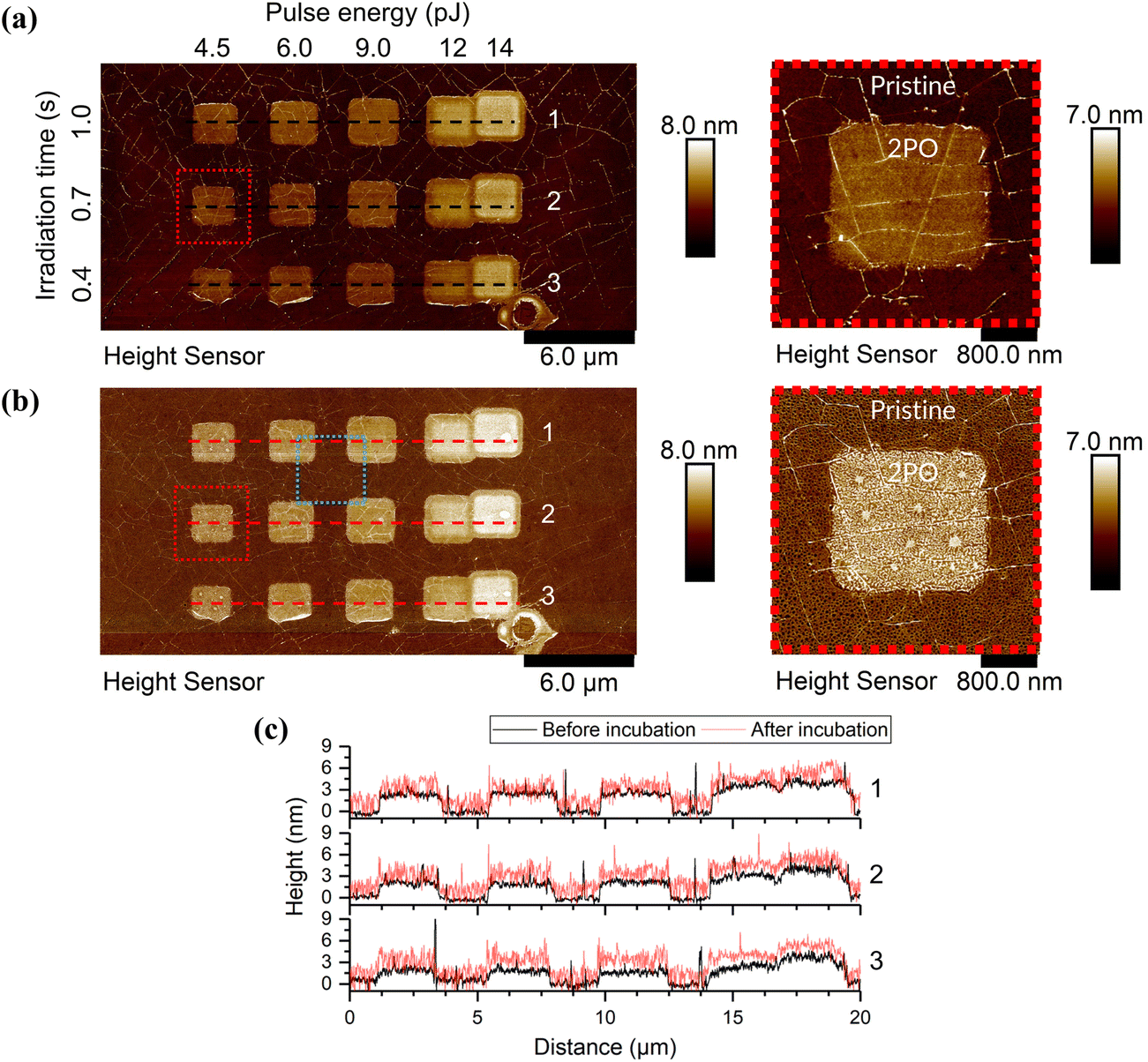

Fig. 1 Topography data of the AFM scans (a) before and (b) after protein incubation in 50 mM PBS, pH 7 and 2.5 μg ml⁻¹ CaM with the areas highlighted in red enlarged on the right to better show the details. The area highlighted in blue is shown enlarged in Fig. 2. The elevated areas were treated with 2PO using the shown parameters, everything else was pristine CVD SLG. See ESI† for all AFM scans of the samples used and their corresponding irradiation parameters. (c) The cross-sections along the dashed lines in the AFM images above for each of the corresponding rows (1–3).

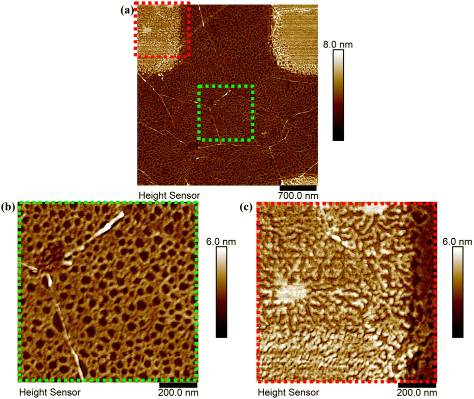Fig. 2 High-resolution images of (a) the area highlighted in blue in Fig. 1 and two further magnified images of areas marked in green (b) (pristine graphene) and red (c) (2PO-treated graphene) to better show the morphology of the protein deposition.

To determine the thickness of the protein layer on top of the pristine graphene, it was assumed that the holes in the network exposed the pristine graphene surface. To support this assumption, a plastic tweezer was used to scratch the sample. An AFM image at the scratch edge was taken, from which either the combined height of the pristine graphene and protein or the height of only the protein layer was measured. It was seen that the protein network did indeed show the pristine graphene surface in the holes of the network (see ESI,† Fig. S7).

In order to verify directly that the immobilized network-like material consisted of proteins, s-SNOM imaging of a sample that was incubated in a 2.5 μg ml⁻¹ mAchR solution (pH 5, 50 mM PBS) was performed. In this technique, the sample was scanned similarly to AFM in tapping mode. During the scan, an IR laser pointed to the AFM tip apex creating a near-field (NF). This NF changed if the incident light frequency is absorbed by the sample. In this way, the optical properties of a sample can be visualized with the spatial resolution of AFM. The method allows the direct correlation of AFM imaging data (Fig. 3(a)) with the optical signal data (Fig. 3(b)). In the experiments presented, the absorption in the amide I frequency range (1645 cm⁻¹) was studied, where all proteins generally show intense absorption bands due to vibration of the C=O groups in their amide backbone.⁵⁹ A higher optical phase (O3P) change in the s-SNOM images coincides with stronger absorption of the incident light. On the sample covered with mAchR, the 2PO areas show a stronger absorption compared to the Pr areas (Fig. 3(b)), indicating a larger number of proteins in these areas, and/or absorption of the 2PO graphene itself at this frequency. However, due to this uncertainty the quantity of protein cannot be determined from the s-SNOM data. Based on the off-resonance image (see ESI† Note 2 and Fig. S8) the latter is at least partially responsible for the larger signal. The higher signal at pristine graphene at off-resonance image could be due to electronic response, which is reduced at the 2PO-treated areas. Also, the graphene wrinkles exhibited a strong signal, which has been previously reported.^60,61

Fig. 3 s-SNOM imaging on a sample incubated in a mAchR solution (2.5 μg ml⁻¹, pH 5). (a) Topography and (b) optical phase (O3P at 1645 cm⁻¹, resonant with the protein) images of the same area. On the right side in both images is a 2PO-treated area with an irradiation dose of 78.4 pJ² s. The highlighted areas are shown enlarged below their corresponding images. The dark red markings highlight similar features of the two images. The profiles along the blue and orange line in the enlarged images of (a) and (b), respectively, are plotted in (c).

When comparing the topography and the optical phase images of a representative pristine area with mAchR, the network structure of the protein layer is visible in both images (enlarged in Fig. 3(a) and (b)) indicating that the immobilized material consists of proteins. A negative control was performed by imaging the same area at 1730 cm⁻¹, which is less resonant to protein vibrations. In the 1730 cm⁻¹ image, the optical phase contrast is lower compared to the image taken at 1645 cm⁻¹, which supports our interpretation (ESI,† Fig. S8).

Cross sections of the topography and optical phase, which is proportional to absorption, of the same pristine area after incubation were compared (Fig. 3(c)). Both profiles follow a similar pattern with only a small deviation, following the results above. Slight deviation of the phases of the profiles could be due to placement error of the profile lines, and topographic effects on the optical signal, where the edges of the proteins could have given distinct signals depending on their position relative to the incident laser beam.⁶² In comparison, in the negative control image (ESI,† Fig. S8) the O3P signal did not follow the height profile at all, which verifies our interpretation of the network consisting of protein. These results demonstrated the great chemical sensitivity of the s-SNOM method as the thickness of the protein layer is roughly 1 nm thick.

A comprehensive analysis of AFM data for each sample consisting of Pr and 2PO-treated areas was performed (ESI,† Fig. S5). Examples of histograms extracted from the data are shown in Fig. 4. The data shows the height distribution of oxidized graphene compared to pristine graphene, and how the protein was distributed on both surfaces. From the analysis, values for the average protein height and coverage were calculated for the Pr and 2PO graphene. For the 2PO square, the edges were ignored as the differences between the edges and the centers of the squares were minuscule and including them would only complicate the analysis.

Fig. 4 Background corrected and normalized height distribution histograms extracted from the AFM images of the highlighted oxidized square area of Fig. 1 (incubated in 50 mM PBS, pH 7 and 2.5 μg ml⁻¹ CaM). The graphs depict the height distributions of Pr graphene surrounding the 2PO square (pristine), 2PO-treated area, and their combined area. Each figure has a percentage value representing the calculated coverage percentage and three histograms that correspond to the same area before protein incubation (initial), after the incubation (incubated) and the calculated overlap between these two histograms (overlap). The combined area histograms are presented in order to show that the background correction has been successful and to highlight that if the Pr and 2PO areas are not treated separately, a significant error in the coverage is introduced, as can be seen from the corresponding coverage percentage values. Corresponding data for each 2PO square of each sample is presented in the ESI.†

3.1. CaM

A summary of the analysis of height histograms for CaM at pH 5, 7, and 9 and with concentrations 0.25 and 2.5 μg ml⁻¹ is presented in Fig. 5, where protein height and coverage are presented for both the pristine graphene (Pr) and the centers of the oxidized squares (2PO). Full histogram data are presented in the ESI† for each sample (Fig. S5). Working at pH 9 proved to be difficult as many of the samples had graphene peel off completely, either during the incubation or rinsing. This can be seen in the AFM images (ESI,† Fig. S6(e) and (i)), where most of the pristine and parts of the oxidized areas have been lifted off. However, it is interesting that the oxidized areas had a higher interaction strength between the substrate and graphene, as the higher oxidation level areas were less likely to detach. In Fig. 5, it is apparent that the oxidation level affects the coverage. This is in accordance to previously reported results that the oxidation level affects the amount of protein adsorbed onto graphene.^31,45 For example, in Fig. 5(b) and (c) the coverage increases from ∼50–60% to 80–90% upon oxidation. In some cases, the effect was weaker or even reversed. For example, in Fig. 5(d), the coverage decreases from ∼70% to ∼55% when the oxidation level is increased at pH 9. It is interesting to correlate the changes in protein coverage to the nature of the oxidized graphene. At low irradiation doses, oxidation occurs at point defect sites.⁴⁸ At higher doses, the point defect density increases until at certain defect density, the defects become line-like or the graphene becomes disordered uniformly.^48,63 It is possible to identify this transition region from Raman spectroscopy.⁶³ The defect concentration induced by 2PO, corresponding to the oxidation level, was determined from Raman spectra from the intensity ratio of the D (∼1350 cm⁻¹) and G (∼1600 cm⁻¹) bands (I_D/I_G). As the oxidation level (defect density) increased, the I_D/I_G ratio first increased. In this region the defects induced were point-like. After the I_D/I_G reached a maximum, it started to decrease when the oxidation level was increased further. This is a turning point where the defects change from the point-like to line-like defects and/or to a uniformly disordered structure.⁶³ This approximate turning point is shown as a vertical dotted line in the plots of Fig. 5. Interestingly, in Fig. 5(b) and (c), corresponding to pH 5 and 7, respectively, the coverage increased upon increasing the defect concentration up to the stage of transition from point defects to disordered material, after which it remains approximately constant. This indicates that at these conditions, oxidized sites at graphene acted as preferential adsorption sites over Pr graphene for CaM. When a high enough dose was used, the graphene structure started to break and became partially or completely ablated. The ablated graphene could be detected when both I_D and I_G became very small or even vanished completely. In a Raman map, the ablated squares showed a lower I_D than the borders of the square, but as the probing spot size partially overlapped with the surrounding pristine or less oxidized graphene, the D, G, and 2D (∼2700 cm⁻¹) bands could still be visible. The values corresponding to ablated squares have been circled in red in Fig. 5. See ESI† for all the Raman maps and their corresponding spectra for each square (Fig. S9†).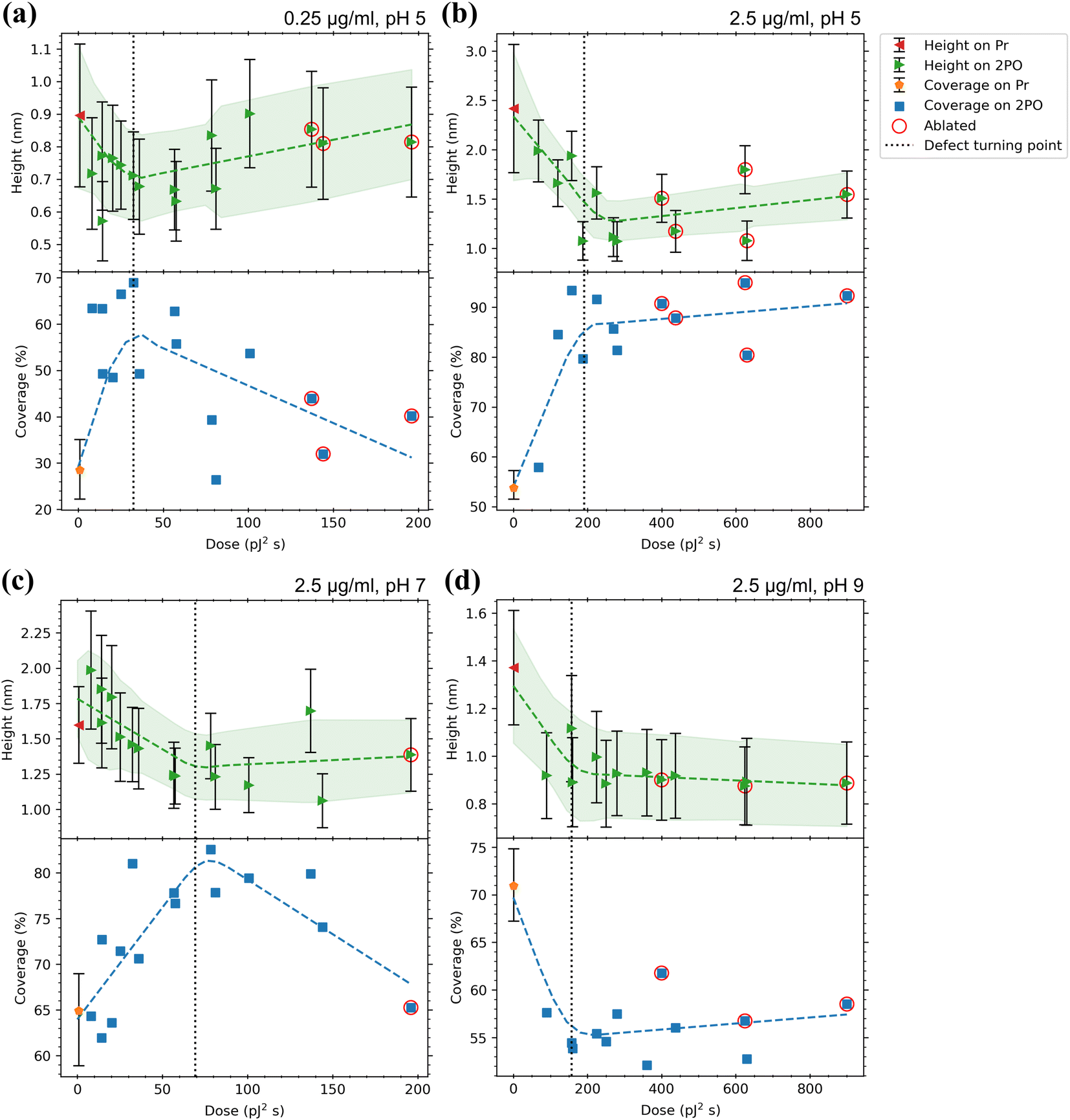

Fig. 5 Adsorption results for CaM with (a) 0.25 μg ml⁻¹, pH 5 (b) 2.5 μg ml⁻¹, pH 5, (c) 2.5 μg ml⁻¹, pH 7 and (d) 2.5 μg ml⁻¹, pH 9 in 50 mM PBS solutions. Top panels indicate the average heights of proteins on both the pristine graphene surrounding the oxidized area (Pr, with the error bars indicating the average of standard deviations of the different areas) and the centers of the oxidized squares (2PO, with the error bars indicating the standard deviation from the Gaussian fits) with a trend line and a confidence interval of one sigma fitted to the data. The bottom panels show the coverage percentages for the same areas with a trend line fitted to the data. For Pr, the error bars indicate the minimum and maximum of the coverages for the different areas. Values for ablated squares are circled in red. The dotted lines indicate the approximate dose where the defects induced by 2PO transition from point-like to line defects as defined by the maximum I_D/I_G ratio. See ESI† for full Raman characterization of the samples.

Height. The protein heights for CaM were all below 3 nm, indicating binding as a monolayer, and the heights showed some dependency on pH and oxidation level. With the lower concentrations used (0.025 μg ml⁻¹ and 0.25 μg ml⁻¹) the height analysis was unreliable and is therefore not emphasized here. This is discussed in the ESI† (ESI Note 3 and Fig. S10). When incubated at 2.5 μg ml⁻¹ and pH 5, (Fig. 5(b)), the average height of CaM on Pr was approximately 2.4 nm. This corresponded well to the dimensions of the reported structure,⁵² which is a somewhat elliptical cylinder shape that is approximately 6.1 nm long, 2.6 nm wide, and 2.1 nm deep. This would indicate that the protein was not distorted and was mostly “lying on its side”. Another report⁶⁴ claims that a height of 2.26 ± 0.21 nm in AFM would correspond to the Ca²⁺ bound conformation of CaM, which the PBS solution did not include. However, on 2PO (2.5 μg ml⁻¹, pH 5) the height decreased to approximately 1–1.5 nm, which is lower than any of the dimensions of the crystalline protein. This could be due to the protein being distorted or partial “embedding” into the oxidized graphene caused by hydrogen bonding of the hydrophilic parts of the protein with the oxygen-containing groups induced in the graphene. The height distribution was broader on the pristine graphene in comparison to the oxidized areas (see ESI,† Fig. S5(c) for details). This could indicate that the protein had a better defined structure on 2PO areas and that the orientation of the protein was more random on the pristine graphene.

At pH 7 (Fig. 5(c)) the protein heights on both Pr and 2PO, approximately 1.6 nm and 1–2 nm, respectively, were smaller than any dimension of the crystalline protein, except at very low oxidation doses. A height of 1.87 ± 0.19 nm has been reported⁶⁴ to correspond to the conformation of CaM when it is not bound to Ca²⁺. A clear saturation level was detected in the protein heights after the approximate defect turning point. Further, at this pH, the height distribution on Pr (Fig. S5(d)†) was a lot sharper than at pH 5. This suggested better defined binding between the protein and the substrate.

For pH 9 (Fig. 5(d)) the heights showed a similar trend as at pH 7 but had even lower values than above (∼1.35 nm (Pr) and 0.9–1.1 nm (2PO)). Low values for both the pristine and oxidized graphene indicated that most probably the protein structure was distorted at this high pH. It is not uncommon for a protein at a pH far away from its pI to have its stability diminished and for denaturation happen at a higher rate.^65–67 The height distributions of the protein on Pr and 2PO (Fig. S5(e)†) were both as sharp as at pH 7.

Coverage. At 0.25 μg ml⁻¹ concentration and pH 5 (Fig. 5(a)) CaM covered 22–35% of Pr graphene and up to 69% of 2PO graphene around the defect turning point. At higher doses the coverage decreased to a minimum of 26%. After increasing the concentration to 2.5 μg ml⁻¹ at pH 5 (Fig. 5(b)), the coverage was still significantly higher for 2PO than for Pr (up to 94% vs. 52%, respectively). The coverage increased within the low (point-defect like) oxidation regime (before the defect turning point) and saturated after reaching the uniformly disordered material regime.

At pH 7 and 2.5 μg ml⁻¹ (Fig. 5(c)), with an increasing oxidation level, the coverage increased from ∼65% (Pr) to a maximum of ∼83% and as highly distorted graphene was reached, the coverage reduced again with the one ablated square having similar coverage as pristine graphene. This seemed to be a unique set of conditions as a saturation level in the coverage was not detected.

For the highest pH and 2.5 μg ml⁻¹ (Fig. 5(d)), the behavior was reversed, as the coverage was consistently around ∼55% for 2PO graphene, whereas for Pr graphene it was around 71%. Based on these coverage results, CaM exhibited clear selectivity towards 2PO over Pr at pH 5. The selectivity at pH 7 was not as strong as at pH 5, and the difference in the minimum to maximum coverage (height of the error bar) on Pr was larger than in the lower pH. The selectivity was reversed at pH 9 as CaM showed selectivity towards pristine graphene. This could be due to both CaM and oxidized graphene becoming negatively charged, leading to electrostatic repulsion, which is absent for Pr graphene. Indeed, the calculated pI for CaM was 4.09, which meant that the protein was negatively charged at all the used pH values, especially at pH 7 and pH 9. At any pH, pristine graphene is hydrophobic and electrostatically neutral. Further, 2PO areas have hydroxyl groups that have a pK_a of 9.32 ± 0.02 (ref. 47) and epoxide rings that reversibly open at alkaline conditions (pH > 7) to produce hydroxyl groups.^42,46 When the rings open, more oxygen attaches to the graphene (ketone opening reaction, C–O–C + OH⁻ + H₂O → 2 C–OH + OH⁻), which in turn makes the surface even more negatively charged at high pH. Therefore, 2PO areas should have been close to neutral at pH 5 and pH 7, and negatively charged at pH 9. This explains the reduction of the coverage of CaM on 2PO at high pH, as both the protein and 2PO graphene both became negatively charged and started to repel each other. The increase in the coverage on Pr graphene could also be explained by the increasingly negative charge of the protein. When the charge is increased, the proteins started to repel each other and prefer the interaction with the neutral pristine graphene. This could also be seen in the AFM images (ESI,† Fig. S6(c–e)), where the height of the protein network decreased as the pH was increased, and the “strings” of the net-like structure widened, which is consistent with the protein having spread more evenly on the graphene surface.

3.2. mAchR

In a similar manner to CaM, a summary of the adsorption analysis results for the mAchR fragment is presented in Fig. 6. The mAchR fragment showed low values for height (≤1.8 nm) on both Pr and 2PO in all the conditions used indicating binding as a monolayer as these values matched reasonably well to the dimensions of a small amino acid chain such as the mAchR fragment. No crystalline structure for this exact fragment is reported in the literature, so more precise comparison could not be performed.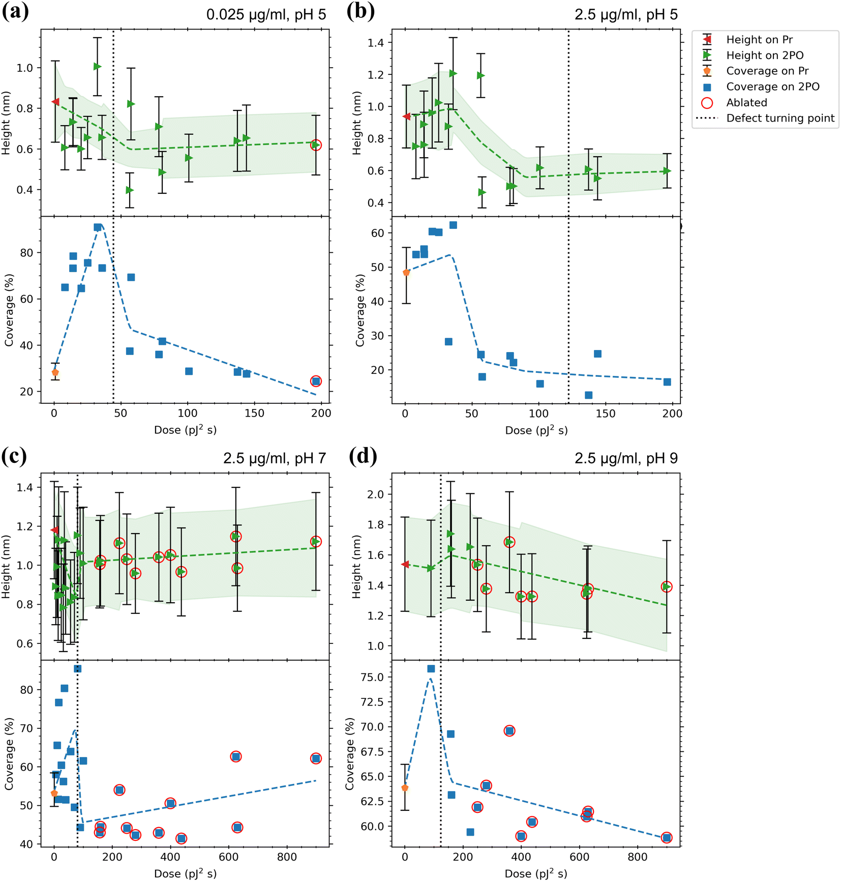

Fig. 6 Adsorption results for mAchR with (a) 0.025 μg ml⁻¹, pH 5, (b) 2.5 μg ml⁻¹, pH 5, (c) 2.5 μg ml⁻¹, pH 7, and (d) 2.5 μg ml⁻¹, pH 9 in 50 mM PBS solutions. Top panels indicate the average heights of proteins on both the pristine graphene surrounding the oxidized area (Pr, where the error bars indicate the average of standard deviations of the different areas) and the centers of the oxidized squares (2PO, where error bars indicate the standard deviation from the Gaussian fits) with a trend line and a confidence interval of one sigma fitted to the data. The bottom panels show the coverage percentages for the same areas with a trend line fitted to the data. For Pr, the error bars indicate the minimum and maximum of the coverages for the different areas. Values for ablated squares are circled in red. The dotted lines indicate the approximate dose where the defects induced by 2PO transition from point-like to line defects defined by the maximum I_D/I_G ratio. See ESI† for full Raman characterization of the samples.

Height. The average height of mAchR on Pr at a concentration of 0.025 μg ml⁻¹ and pH 5 (Fig. 6(a)) was approximately 0.85 nm and the height decreased to approximately 0.65 nm with low oxidation doses. When the approximate defect turning point was approached, the spread of different heights became relatively large (0.4–1.0 nm) and converged at high doses, where the heights settled at approximately 0.6 nm. When the concentration was increased to 2.5 μg ml⁻¹ (Fig. 6(b)), the average height on Pr graphene was approximately 0.95 nm and on 2PO graphene the heights were approximately 0.5–1.2 nm. A significant drop in the average protein height was detected with doses higher than 30 pJ² s. Below this dose, the oxidation level is so low that the oxidized squares are hardly visible in the AFM images (ESI,† Fig. S6(g)). Therefore, the histograms below and above the dose of 30 pJ² s are very different (ESI,† Fig. S5(g)), which may partially explain the large drop in the height values. However, the Raman spectra show similar trend as for all samples, namely monotonous increase of defects by increasing irradiation dose. Therefore, even though the AFM image differs from other samples, the Raman data shows that the 2PO process worked similarly for all samples.

When incubated at pH 7 and 2.5 μg ml⁻¹ (Fig. 6(c)) the protein heights on Pr were a bit larger (∼1.2 nm) compared to pH 5. On 2PO graphene, there was less spread in the heights, but the maximum height was almost the same (∼1.15 nm (pH 7) vs. ∼1.2 nm (pH 5)). The initial rise from the Pr height was not observed. Instead, the low oxidation doses lowered the average height, which then increased again with higher doses.

At pH 9 and 2.5 μg ml⁻¹ (Fig. 6(d)) the protein heights were larger than at lower pH values, not only on Pr graphene but this time also on the 2PO graphene (∼1.35 nm (Pr) and 1.30–1.75 nm (2PO)). Unfortunately, the areas with the lowest doses used at this pH were lost due to them lifting off, as discussed above with CaM, so there is a notable lack of datapoints in the region between the pristine graphene and the approximate defect turning point. Additionally, no significant initial drop in the heights was seen, but after crossing the approximate defect turning point, a small increase in the heights was present, after which the heights dropped again and saturated around 1.3 to 1.4 nm.

Coverage. At 0.025 μg ml⁻¹ and pH 5 mAchR covered 29% of Pr and the coverage increased with oxidation dose until it reached the highest coverage of 91% at a dose of 32.4 pJ² s. With higher doses past the defect turning point, the coverage reduced again down to 24%. Thus, at low oxidation levels, there was notable selectivity towards oxidized areas in comparison to the Pr. At the concentration of 2.5 μg ml⁻¹ at pH 5, Pr coverage was 48%, which increased with very low oxidation levels up to 62%. Past the dose of 30 pJ² s, the coverage dropped suddenly, similarly to the trend seen for the height. Also in this case, the large qualitative change in the histograms (ESI,† Fig. S5(g)) may partially explain the large sudden drop. For higher irradiation doses, the coverage reached a minimum of 12.6% around the approximate defect turning point. This indicated clear selectivity towards the pristine or low oxidation level graphene. At the low concentration (0.025 μg ml⁻¹) the selectivity of the coverage was better than at the higher concentration (2.5 μg ml⁻¹), which is understandable since at very high concentrations protein would probably cover all surfaces, which corresponds to total loss of selectivity.

In comparison to the lower pH, the Pr coverage slightly increased (to 53%) at pH 7 and 2.5 μg ml⁻¹. At low levels of oxidation, the coverage increased and reached a maximum value of 85.5% at the defect turning point, after which the coverage decreased to a minimum of 41%.

After incubation at pH 9, the Pr coverage increased to approximately 64% and the highest coverage with 2PO, again near the defect turning point, reduced to 76% compared to the lower pH. When the oxidation level was increased further, the coverage decreased to 59%. mAchR behaved in a very similar way at both pH 7 and 9. The highest coverage was detected at low oxidation levels and as the oxidation level was increased, a saturation level was reached, although this is not as clear at pH 9. The calculated pI for mAchR (4.57) was similar to CaM. Therefore, the mAchR fragment was negatively charged in all the pH used and the negative charge likely intensified when the pH was increased, just like with CaM. Thus, the behavior was expected to be similar, which—at least with the coverage—was the case. Although the effect was not as strong as with CaM, as the pH was increased, the mAchR coverage on Pr graphene increased and the highest detected coverage on 2PO graphene decreased. These trends could be partially explained by the electrostatic effect, as described previously. The repulsion between the charged proteins could have favored the protein spreading more evenly on the Pr graphene, which could be seen as the increase of the standard deviation (magnitude of the height error bars, Fig. 6(d)).

3.3. Outlook

All the data presented here show that the best selectivity is achieved with low oxidation levels (i.e., the point-like defect regime). This is also promising for future applications of 2PO and controlling protein adsorption onto graphene, as within this region, the graphene is still of good quality and conductive and therefore good for electronic devices and sensors. Other proteins have been shown to preserve their secondary structure⁶⁸ and stay active when adsorbed to graphene⁶⁹ or to other graphene-based materials.³⁹ However, the topic is controversial as some proteins have been claimed to lose their biological function when physically adsorbed to graphene without any intermediate layer.²⁴ If the methods described here work for proteins that specifically bind to NTs, such as mAchR, or other neurotransmission-relevant proteins like CaM and the proteins maintain their biological function (as reported before^36,39,69), biosensor devices functionalized with proteins can have very local control of adsorption thanks to 2PO, limited only by the dimensions of the irradiation area. Additionally, using 2PO is a relatively simple method of controlling the area-specific binding. This can lead to smaller graphene-based devices with individually functionalized areas very close to each other, which in turn makes more specific and local sensing possible. For neuroapplications this can be very significant. When successful, it offers less invasive methods of measuring the neural signals meant for e.g., muscle movement. Compare, for example, the invasiveness of implanting a device on the nerves in the arm instead of using an intracortical electrode. Thus, the present results are promising for developing functionalized graphene-based biosensor devices for measurement of neuronal activity at high spatial resolution.

Conclusions

We have demonstrated that 2PO can be utilized to affect adsorption of neurotransmission-relevant proteins on graphene. The proteins predominantly bind in a monolayer, and no evidence of thicker layers was observed at the studied concentrations. The extremes of selectivity between pristine and laser-oxidized graphene for mAchR varied from 29% (Pr) vs. 91% (2PO) to 48% (Pr) vs. 13% (2PO) surface area covered and for CaM from 53% (Pr) vs. 95% (2PO) to 71% (Pr) vs. 52% (2PO) surface area covered. The most significant impact on selectivity occurred in the point-like defect regime, i.e., at low oxidation levels. At higher oxidation levels, when graphene became disordered and eventually ablated, the selectivity of the adsorption was partially lost. By selecting the appropriate conditions, a high selectivity can be achieved for both proteins. Additionally, the selectivity towards pristine or oxidized graphene can be precisely controlled via immobilization conditions and laser dose. Some conditions showed indications of protein structure distortion. The behavior as a function of the oxidation level depended on the protein and its structure, pH, and the protein concentration used.

Employing the methods described here allows for the straightforward fabrication of specific graphene-based biosensors. The use of readily available and relatively inexpensive proteins or their fragments has proven to be a cost-effective and valuable approach for the initial investigation of this functionalization method. It holds promise for future biosensing measurements and the utilization of more complex biologically functional proteins.

Data availability

The data supporting this article have been included as part of the ESI.† The original files are available upon request from the corresponding author.

Author contributions

A. L. conducted the adsorption experiments, Raman and AFM characterization, data analysis, and analysis related programming, developed the AFM analysis method, and wrote the original manuscript. J. S. conducted the s-SNOM experiments, took part in designing the adsorption experiments and wrote the s-SNOM sections of the original draft. A. E. conducted the graphene oxidation and part of the Raman measurements. A. J. and M. P. supervised the research. M. P. administered the project. A. L., J. S., A. E., A. J., and M. P. contributed to the discussion and manuscript editing.

Conflicts of interest

There are no conflicts to declare.

Acknowledgements

The authors acknowledge Olli Rissanen for the valuable technical work with sample and graphene fabrication, Eero Hulkko for the practical help in s-SNOM measurements, Erich See for the discussions and proofreading, Astrid Mayné and Laura Bono Ros for their efforts in the initial studies, and ChatGPT, which was used to improve upon the grammar and flow of the text when working on the initial draft. Also, we thank Emil Aaltonen foundation and Jane and Aatos Erkko foundation for the research funding provided.

References

1. S. E. Hyman, Curr. Biol., 2005, 15, R154–R158.
2. A. E. Pereda, Nat. Rev. Neurosci., 2014, 15, 250.
3. E. M. Tansey, C. R. Biol., 2006, 329, 419–425.
4. A. C. Kruse, B. K. Kobilka, D. Gautam, P. M. Sexton, A. Christopoulos and J. Wess, Nat. Rev. Drug Discovery, 2014, 13, 549–560.
5. J. Wess, R. M. Eglen and D. Gautam, Nat. Rev. Drug Discovery, 2007, 6, 721–733.
6. C. Gotti, F. Clementi, A. Fornari, A. Gaimarri, S. Guiducci, I. Manfredi, M. Moretti, P. Pedrazzi, L. Pucci and M. Zoli, Biochem. Pharmacol., 2009, 78, 703–711.
7. M. Zoli, S. Pucci, A. Vilella and C. Gotti, Curr. Neuropharmacol., 2018, 16, 338.
8. Q. Huang, C. Liao, F. Ge, J. Ao and T. Liu, J. Neurorestoratol., 2022, 10, 100002.
9. R. Rudolf and T. Straka, Neurosci. Lett., 2019, 711, 134434.
10. M. E. J. Obien, K. Deligkaris, T. Bullmann, D. J. Bakkum and U. Frey, Front. Neurosci., 2015, 9, 423.
11. B. Pesaran, M. Vinck, G. T. Einevoll, A. Sirota, P. Fries, M. Siegel, W. Truccolo, C. E. Schroeder and R. Srinivasan, Nat. Neurosci., 2018, 21, 903–919.
12. W. Wei and X. Wang, Materials, 2021, 14, 6170.
13. L. J. A. Macedo, R. M. Iost, A. Hassan, K. Balasubramanian and F. N. Crespilho, ChemElectroChem, 2019, 6, 31–59.
14. H. Huang, S. Su, N. Wu, H. Wan, S. Wan, H. Bi and L. Sun, Front. Chem., 2019, 7, 464141.
15. M. J. Allen, V. C. Tung and R. B. Kaner, Chem. Rev., 2010, 110, 132–145.
16. P. Suvarnaphaet and S. Pechprasarn, Sensors, 2017, 17, 2161.
17. I. Fakih, O. Durnan, F. Mahvash, I. Napal, A. Centeno, A. Zurutuza, V. Yargeau and T. Szkopek, Nat. Commun., 2020, 11, 3226.
18. N. Alzate-Carvajal and A. Luican-Mayer, ACS Omega, 2020, 5, 21320–21329.
19. G. Xu, Z. A. Jarjes, V. Desprez, P. A. Kilmartin and J. Travas-Sejdic, Biosens. Bioelectron., 2018, 107, 184–191.
20. D. M. Goodwin, F. Walters, M. M. Ali, E. Daghigh Ahmadi and O. J. Guy, Chemosensors, 2021, 9, 174.
21. Z. Gu, Z. Yang, L. Wang, H. Zhou, C. A. Jimenez-Cruz and R. Zhou, Sci. Rep., 2015, 5, 1–11.
22. S. R. Shin, Y. C. Li, H. L. Jang, P. Khoshakhlagh, M. Akbari, A. Nasajpour, Y. S. Zhang, A. Tamayol and A. Khademhosseini, Adv. Drug Delivery Rev., 2016, 105, 255–274.
23. S. C. Smith, F. Ahmed, K. M. Gutierrez and D. Frigi Rodrigues, Chem. Eng. J., 2014, 240, 147–154.
24. T. Alava, J. A. Mann, C. Théodore, J. J. Benitez, W. R. Dichtel, J. M. Parpia and H. G. Craighead, Anal. Chem., 2013, 85, 2754–2759.
25. C. J. Russo and L. A. Passmore, Nat. Methods, 2014, 11, 649–652.
26. Y. Kamiya, K. Yamazaki and T. Ogino, J. Colloid Interface Sci., 2014, 431, 77–81.
27. K. Chaudhary, K. Kumar, P. Venkatesu and D. T. Masram, Adv. Colloid Interface Sci., 2021, 289, 102367.
28. P. C. Henriques, A. T. Pereira, A. L. Pires, A. M. Pereira, F. D. Magalhães and I. C. Gonçalves, ACS Appl. Mater. Interfaces, 2020, 12, 21020–21035.
29. C. H. Lu, C. L. Zhu, J. Li, J. J. Liu, X. Chen and H. H. Yang, Chem. Commun., 2010, 46, 3116–3118.
30. D. L. de Sousa Maia, F. Côa, K. B. da Silva, C. H. Z. Martins, L. S. Franqui, L. C. Fonseca, D. S. da Silva, F. de Souza Delite, D. S. T. Martinez and O. L. Alves, J. Mater. Sci., 2024, 59, 577–592.
31. Y. Qi, W. Chen, F. Liu, J. Liu, T. Zhang and W. Chen, Environ. Sci.: Nano, 2019, 6, 1303–1309.
32. H. Li, K. Fierens, Z. Zhang, N. Vanparijs, M. J. Schuijs, K. Van Steendam, N. Feiner Gracia, R. De Rycke, T. De Beer, A. De Beuckelaer, S. De Koker, D. Deforce, L. Albertazzi, J. Grooten, B. N. Lambrecht and B. G. De Geest, ACS Appl. Mater. Interfaces, 2016, 8, 1147–1155.
33. Z. Tang, H. Wu, J. R. Cort, G. W. Buchko, Y. Zhang, Y. Shao, I. A. Aksay, J. Liu and Y. Lin, Small, 2010, 6, 1205–1209.
34. R. Chai, C. Xing, D. Gao, H. Yuan, Y. Zhan and S. Wang, Adv. Healthcare Mater., 2018, 7, 1800674.
35. Q. He, H. G. Sudibya, Z. Yin, S. Wu, H. Li, F. Boey, W. Huang, P. Chen and H. Zhang, ACS Nano, 2010, 4, 3201–3208.
36. H. G. Sudibya, Q. He, H. Zhang and P. Chen, ACS Nano, 2011, 5, 1990–1994.
37. M. Feng, D. R. Bell, J. Luo and R. Zhou, Phys. Chem. Chem. Phys., 2017, 19, 10187–10195.
38. J. Gao, L. Wang, S. G. Kang, L. Zhao, M. Ji, C. Chen, Y. Zhao, R. Zhou and J. Li, Nanoscale, 2014, 6, 12828–12837.
39. B. Kim, H. S. Song, H. J. Jin, E. J. Park, S. H. Lee, B. Y. Lee, T. H. Park and S. Hong, Nanotechnology, 2013, 24, 285501.
40. D. C. Marcano, D. V. Kosynkin, J. M. Berlin, A. Sinitskii, Z. Sun, A. Slesarev, L. B. Alemany, W. Lu and J. M. Tour, ACS Nano, 2010, 4, 4806–4814.
41. J. Aumanen, A. Johansson, J. Koivistoinen, P. Myllyperkiö and M. Pettersson, Nanoscale, 2015, 7, 2851–2855.
42. A. Johansson, H. C. Tsai, J. Aumanen, J. Koivistoinen, P. Myllyperkiö, Y. Z. Hung, M. C. Chuang, C. H. Chen, W. Y. Woon and M. Pettersson, Carbon, 2017, 115, 77–82.
43. A. V. Emelianov, D. Kireev, A. Offenhäusser, N. Otero, P. M. Romero and I. I. Bobrinetskiy, ACS Photonics, 2018, 5, 3107–3115.
44. A. Lampinen, E. See, A. Emelianov, P. Myllyperkiö, A. Johansson and M. Pettersson, Phys. Chem. Chem. Phys., 2023, 25, 10778–10784.
45. E. D. Sitsanidis, J. Schirmer, A. Lampinen, K. K. Mentel, V. M. Hiltunen, V. Ruokolainen, A. Johansson, P. Myllyperkiö, M. Nissinen and M. Pettersson, Nanoscale Adv., 2021, 3, 2065–2074.
46. T. Taniguchi, S. Kurihara, H. Tateishi, K. Hatakeyama, M. Koinuma, H. Yokoi, M. Hara, H. Ishikawa and Y. Matsumoto, Carbon, 2015, 84, 560–566.
47. E. S. Orth, J. G. L. Ferreira, J. E. S. Fonsaca, S. F. Blaskievicz, S. H. Domingues, A. Dasgupta, M. Terrones and A. J. G. Zarbin, J. Colloid Interface Sci., 2016, 467, 239–244.
48. J. Koivistoinen, L. Sládková, J. Aumanen, P. Koskinen, K. Roberts, A. Johansson, P. Myllyperkiö and M. Pettersson, J. Phys. Chem. C, 2016, 120, 22330–22341.
49. K. K. Mentel, A. V. Emelianov, A. Philip, A. Johansson, M. Karppinen and M. Pettersson, Adv. Mater. Interfaces, 2022, 9, 2201110.
50. R. Tilmann, C. Bartlam, O. Hartwig, B. Tywoniuk, N. Dominik, C. P. Cullen, L. Peters, T. Stimpel-Lindner, N. McEvoy and G. S. Duesberg, ACS Nano, 2023, 17, 10617–10627.
51. X. Díez-Betriu, S. Álvarez-García, C. Botas, P. Álvarez, J. Sánchez-Marcos, C. Prieto, R. Menéndez and A. De Andrés, J. Mater. Chem. C, 2013, 1, 6905–6912.
52. S. T. Rao, S. Wu, K. A. Satyshur, M. Sundaralingam, K.-Y. Ling and C. Kung, Protein Sci., 1993, 2, 436–447.
53. K. Haga, A. C. Kruse, H. Asada, T. Yurugi-Kobayashi, M. Shiroishi, C. Zhang, W. I. Weis, T. Okada, B. K. Kobilka, T. Haga and T. Kobayashi, Nature, 2012, 482, 547–551.
54. J. Grobelny, F. W. DelRio, P. Namboodiri, D.-I. Kim, V. A. Hackley and R. F. Cook, Size Measurement of Nanoparticles using Atomic Force Microscopy, https://www.nist.gov/publications/size-measurement-nanoparticles-using-atomic-force-microscopy, (accessed 6 February 2024).
55. D. Sehnal, S. Bittrich, M. Deshpande, R. Svobodová, K. Berka, V. Bazgier, S. Velankar, S. K. Burley, J. Koča and A. S. Rose, Nucleic Acids Res., 2021, 49, W431–W437.
56. F. Bathawab, M. Bennett, M. Cantini, J. Reboud, M. J. Dalby and M. Salmerón-Sánchez, Langmuir, 2016, 32, 800–809.
57. M. T. Hwang, B. L. Preston, L. Joon, C. Duyoung, H. M. Alexander, G. Gennadi and L. Ratnesh, Proc. Natl. Acad. Sci. U. S. A., 2016, 113, 7088–7093.
58. S. L. Baltierra-Uribe, J. J. Chanona-Pérez, J. V. Méndez-Méndez, M. D. J. Perea-Flores, A. C. Sánchez-Chávez, B. E. García-Pérez, M. C. Moreno-Lafont and R. López-Santiago, Microsc. Res. Tech., 2019, 82, 586–595.
59. A. Barth, Biochim. Biophys. Acta, Bioenerg., 2007, 1767, 1073–1101.
60. H. Wang, L. Wang, D. S. Jakob and X. G. Xu, AIP Adv., 2017, 7, 55118.
61. J. Schirmer, R. Chevigny, A. Emelianov, E. Hulkko, A. Johansson, P. Myllyperkiö, E. D. Sitsanidis, M. Nissinen and M. Pettersson, Phys. Chem. Chem. Phys., 2023, 25, 8725–8733.
62. L. Mester, A. A. Govyadinov and R. Hillenbrand, NANO, 2022, 11, 377–390.
63. L. G. Cançado, A. Jorio, E. H. M. Ferreira, F. Stavale, C. A. Achete, R. B. Capaz, M. V. O. Moutinho, A. Lombardo, T. S. Kulmala and A. C. Ferrari, Nano Lett., 2011, 11, 3190–3196.
64. S. Trajkovic, X. Zhang, S. Daunert and Y. Cai, Langmuir, 2011, 27, 10793–10799.
65. K. A. Dill and D. Shortie, Annu. Rev. Biochem., 1991, 60, 795–825.
66. A. J. R. Law and J. Leaver, J. Agric. Food Chem., 2000, 48, 672–679.
67. H. Saito, M. Takase, Y. Tamura, S. Shimamura and M. Tomita, Adv. Exp. Med. Biol., 1994, 357, 219–226.
68. J. G. Vilhena, P. Rubio-Pereda, P. Vellosillo, P. A. Serena and R. Pérez, Langmuir, 2016, 32, 1742–1755.
69. J. Schirmer, E. Iatta, A. V. Emelianov, M. Nissinen and M. Pettersson, Adv. Mater. Interfaces, 2023, 11, 2300870.

---

Footnote

† Electronic supplementary information (ESI) available: All sample 2PO and adsorption conditions, detailed description and discussion on the AFM analysis method used, full height distribution histogram data, all AFM images, example scratch test data, all Raman maps and spectra, s-SNOM negative control data, and outlier low concentration adsorption data. See DOI: https://doi.org/10.1039/d4lf00102h

---