Sequence determinants of protein phase separation and recognition by protein phase-separated condensates through molecular dynamics and active learning

Abstract

Elucidating how protein sequence determines the properties of disordered proteins and their phase-separated condensates is a great challenge in computational chemistry, biology, and biophysics. Quantitative molecular dynamics simulations and derived free energy values can in principle capture how a sequence encodes the chemical and biological properties of a protein. These calculations are, however, computationally demanding, even after reducing the representation by coarse-graining; exploring the large spaces of potentially relevant sequences remains a formidable task. We employ an “active learning” scheme introduced by Yang et al. (bioRxiv, 2022, https://doi.org/10.1101/2022.08.05.502972) to reduce the number of labelled examples needed from simulations, where a neural network-based model suggests the most useful examples for the next training cycle. Applying this Bayesian optimisation framework, we determine properties of protein sequences with coarse-grained molecular dynamics, which enables the network to establish sequence–property relationships for disordered proteins and their self-interactions and their interactions in phase-separated condensates. We show how iterative training with second virial coefficients derived from the simulations of disordered protein sequences leads to a rapid improvement in predicting peptide self-interactions. We employ this Bayesian approach to efficiently search for new sequences that bind to condensates of the disordered C-terminal domain (CTD) of RNA Polymerase II, by simulating molecular recognition of peptides to phase-separated condensates in coarse-grained molecular dynamics. By searching for protein sequences which prefer to self-interact rather than interact with another protein sequence we are able to shape the morphology of protein condensates and design multiphasic protein condensates.

---

1 Introduction

Proteins and other biomolecules within cells can phase separate to form liquid-like droplets.¹ Such phase-separated droplet regions provide a unique microenvironment essential for several important cellular processes and thus are an important way of regulating biological function. The human proteome has a very rich diversity in terms of composition.² A predictive insight into which protein sequences could undergo phase-separation would improve understanding of the pathogenesis of several neurodegenerative diseases including Alzheimer’s disease,^3,4 where protein phase separation and the formation of toxic aggregates of these proteins have been linked to pathogenesis. Different condensates or condensates with multiple distinct phases provide a way for biological processes to be regulated in time and space.^5–7 Spatially separating different biochemical reactions is also a promising blueprint for biotechnological applications.⁸ This necessitates efficient strategies to design novel phase separating condensates and to develop molecules, such as artificial proteins, to bind selectively to phase-separated condensates. However, in other contexts such as designing protein interaction modules for synthetic biology,⁹ one might specifically want to reduce the propensity of proteins to interact and form condensates.

Molecular dynamics (MD) simulations have played a major role in our understanding of protein–protein interactions and protein phase separation.^1,10–12 The development of state-of-the-art molecular force fields has enabled accurate representation of molecular interactions, allowing these simulation models to successfully predict phase separation propensities of diverse protein sequences.^11,13 Atomistic molecular dynamics simulations can provide essential insights into molecular driving forces by simplifying the description. However, building an exact quantitative understanding of a protein sequence–property relationship, to be able to predict the behaviour of a sequence without the necessity of a simulation or an experiment, has remained difficult to achieve. This is in part due to the large space of possible biological sequences, and also how sequence context will change the interaction characteristics of the amino acids.

One way to model such complicated relationships is via machine learning, and recently, important progress has been made in learning such relationships and also applying this progress to the interactions and phase behaviour of flexible and disordered proteins.^14–17 A very successful strategy has been to combine physics-based simulations with machine learning and artificial intelligence.^16,18,19 Ginell et al. have trained a neural network with a physics-based simulation model to predict how different disordered proteins will interact.¹⁴ With a physics-based simulation model von Bülow et al. have successfully trained a neural network to predict the phase separation propensities of proteins.¹⁵ In recent years, protein language models have been shown to organise protein sequences in biologically meaningful ways.^20–23 Language models also seem to encode useful physical and chemical information, which makes it imperative to see how we can leverage the information encoded in such models to predict protein behaviour. Language models have been used in iterative design²⁴ and for proposing entirely novel proteins.²³ However, a key difficulty in mapping sequence–property relationships is the limited availability of “labelled” data needed for training. The property of interest may require experimental input or computationally expensive simulations. One must also note that not all labelled data is equally useful, and some specific examples may be more beneficial for training than others.

Active learning²⁷ is a machine learning paradigm meant to address exactly this issue, where the model interacts with the human to suggest which labelled examples should be provided for training. Within such a framework, Bayesian Optimisation (BO) can be invoked to rank the most useful sequences in terms of their potential utility to the model and thus can be used to judiciously direct one’s resources. These approaches can be utilised to understand how chemical structure and biological sequences give rise to chemical²⁸ and biological properties. Recently, An et al.²⁹ used active learning to discover strongly interacting proteins that tend to phase-separate, while optimising the trade-off between thermodynamic stability and transport properties. In another context, it was demonstrated that active learning helps to design molecules selectively interacting with one phase of a lipid membrane over another phase of this membrane³⁰ and to find small molecules binding to a protein.³¹ Chemical structure and biological sequences have to be inputted in a way that is amenable to machine learning. One possibility is to combine various metrics. Deep learning provides a way of achieving this and promising results based on autoencoder have been obtained.³⁰ For biological sequences, language models may be a natural way of representing sequences and recent advances make it possible to use pre-trained language models for featurisation.^24,25 Language models show a lot of promise for BO, as exemplified by a recent study by Hoffbauer and Strodel,¹⁷ where the authors showed that the biochemical knowledge encoded in an advanced pre-trained language model enables efficient active learning even when only limited data is available. Yang et al. have developed a very promising workflow based on a pre-trained language model²⁵ and deep ensembles to express the learned relationships. Here we investigated three related questions: (1) Can we identify the sequence determinants which lead to protein self interactions and phase separation? (2) Can we understand and design new sequences which selectively bind to phase-separated protein condensates? (3) Can we design multiphasic condensates? To address these important questions in biophysics and physical chemistry we utilize the BO approach by Yang et al.²⁵ (Fig. 1).

Fig. 1 Schematic overview of the active learning framework for predicting peptides using Bayesian Optimisation (BO) and Molecular Dynamics (MD) simulations: (A) MD simulations of protein chains to compute second virial coefficient (B₂₂) and partition free energy (ΔG) for model training. This initial sample is fed to the BO package,²⁵ which utilises UniRep LSTM,^24,26 to parse the protein sequence into a feature vector . Deep ensemble training on feature vectors and computed properties to establish sequence–property relationships. To choose which sequences the model would benefit the most from, an acquisition function is used to rank and suggest the next set of sequences. The suggested sequences are simulated again, generating new data for subsequent training cycles. This iterative process helps the model learn the sequence–property relationship with fewer examples and simultaneously explore sequence space regions that contain proteins with the most extreme values of the property we studied.

2 Methods

We study the mapping of a protein sequence to one of its properties, as represented by a numeric quantity . As we shall describe later, f(x) could be the second virial coefficient B₂₂, or another quantity that provides an estimate of the affinity of a sequence to bind to a condensate. Our scientific problem thus reduces to training a model to learn the mapping between and , while simultaneously exploring the protein sequence space to maximise this label. We utilize the package²⁵ which provides the framework for performing such optimisation tasks implemented here.

Fig. 1 illustrates our workflow: We begin with an initial set of protein sequences and conduct coarse-grained molecular dynamics simulations to extract for instance, B₂₂ or ΔG values. We initialize a surrogate model within the protein sequence Bayesian Optimisation (BO) package ²⁵ and provide it with an initial set of sequences and labels to calibrate the initial sequence–property mapping. During that, uses UniRep—a multiplicative Long-Short Term Memory (mLSTM) model^24,26 for parsing the amino acid sequence into a feature vector x that contains the essential protein features in a fixed-length numeric vector.

UniRep, trained on 24 million primary amino acid sequences in the UniRef50 database, has shown the ability to accurately partition structurally and evolutionarily similar proteins, even when they share little sequence identity.²⁴ The resulting feature vectors, combined with the computed labels, serve as input for training the surrogate models, which in the context of are ensembles of multi-layer perceptrons (MLPs). Such deep ensembles are appropriate for uncertainty quantification and offer greater expressive power compared to the Gaussian processes (GPs) that are otherwise typically chosen as surrogates.

Following this initial calibration of sequence–property mapping, the Bayesian optimiser uses an acquisition function to rank which proteins would serve as the most useful examples for further training. This process simultaneously explores the sequence space, in search of regions with proteins that possess the highest values of the property we are studying. A batch of sequences is drawn from this for the next cycle of training. Coarse-grained simulations of these sequences are again performed, and the entire process is repeated for several iterations. In the subsequent sections, we provide a detailed account of the training and optimisation methodology.

2.1 Model description and optimisation

As mentioned before, the surrogate model in is an ensemble of feedforward neural networks (called a deep ensemble³²). In such a model, the quantity of interest f(x) is independently predicted by not one but an ensemble of neural network models, which in this case is a Multi-Layer Perceptron (MLP). In the configuration used here, the ensemble comprises of 5 MLPs. UniRep²⁴ parses an input sequence into a fixed-length feature vector of dimension N = 1900. Therefore, each individual MLP takes an input of dimension 1900, followed by three layers having 128, 32, and 2 neurons each. The last layer outputs two numbers: a mean [small mu, Greek, circumflex] and a standard deviation [small sigma, Greek, circumflex] that characterise a normal distribution . The dispersion in the mean values [small mu, Greek, circumflex] predicted by the individual models, and the sum of the variances [small sigma, Greek, circumflex]² of this by the different models, together give a total uncertainty estimate. All networks layer but the last one is followed with the SiLU (also known as Swish) activation function. In addition, standard techniques such as dropout and weight decay are utilised to reduce overfitting. For further technical description about , we refer the reader to Yang et al., who designed it.²⁵

The advantage of deep ensembles is that neural networks possess more expressive power than Gaussian processes, while providing a way of uncertainty quantification. Bayesian optimisation works via ranking sequences using an acquisition function . Unless stated otherwise, for most of the work presented here, we chose the “upper confidence bound” (UCB) acquisition function³³ which balances both exploitation of the known maximas and exploration of the parameter space:

here, the exploitation term μ(x), represents the current estimate of the value known to the surrogate, while the exploration term σ(x) quantifies the uncertainty. The parameter λ acts as a control to adjust the balance between exploitation and exploration. λ is set to a value 2.

Another commonly used acquisition function is Expected Improvement (EI). The fundamental principle behind EI is to select the next point to evaluate based on the current best result. The choice of the acquisition function sensitively affects which regions of sequence space get explored for, and thus the arrival at, an optimal solution. Later, in Section 3.1, we will show the impact of this choice as observed in our study.

2.2 Training and validation

Optimisation of the surrogate model—by asking it to suggest sequences to be measured in a lab or simulated—requires an initial calibration. For most of the tasks studied here, an initial set of sequences was drawn from ProtGPT2,²³ a protein language model constructed for de novo protein design. Quantities f(x), either B₂₂ or ΔG values, were computed from coarse-grained molecular dynamics. This computed value was treated as the true or expected value of the property of interest. The length of all sequences used for training was chosen to be 21 amino acids.

While training, to track the learning of the model, we set aside two sets of sequences for validation of the model’s predictive ability, which were never used for training. The first set was drawn the same way as the training data itself, with 42 21-amino acid length sequences drawn from the ProtGPT2 language model,²³ spanning a wide range of B₂₂ values. To track how well the approach captures strongly interacting peptides which are likely only a small fraction of natural protein sequences, we generated a second set of validation data. We took 22 21-amino acid sequences with very negative B₂₂ values from the study of An et al. (2024)²⁹ (see their ESI Tables). The true values of B₂₂ for these validation sequences were computed in exactly the same way, from coarse-grained simulations. The coarse-grained simulations for calculating B₂₂ were conducted for 10 μs.

For designing peptides that bind to condensates, an initial calibration set of 70 21-mer peptides was selected from An et al. (2024). For validation, 30 peptides were chosen from ProtGPT2. The simulations involving the condensate and peptides were performed for 0.6 μs.

Similar to Yang et al.,²⁵ we will refer to an “optimisation step” as being the usage of one sequence-label pair after which the model is updated. Subsequent to each optimisation step, we predicted the numeric label for the validation set sequences and tracked the mean squared error from the residual between true (computed from simulations) and values predicted by the model. The exact size of the calibration and validation sets were chosen separately for the different tasks studied here (described in their respective subsections). In all that follows, we shall refer to the initial calibration as iteration 0.

2.3 Specifications of the coarse-grained molecular dynamics simulations

Residue-level coarse-grained simulations with the HPS model³⁴ were run in HOOMD-blue v. 2.9.6 ³⁵ extended with azplugins (v. 2.9.2). Simulations were also conducted with the more recent CALVADOS2 simulation model.¹³ The second virial coefficient (B₂₂) was calculated from the simulations of two 21-amino acid peptide sequences in a cubic box of dimension 8 nm × 8 nm × 8 nm. To determine the partition free energy, condensate simulations were conducted in a slab geometry of dimension 15 × 15 × 250 nm. The condensate was simulated with 300 chains of 140-amino acid CTD of RNA Polymerase II, and 30 chains of 21-amino acid peptides were added to the preformed condensate.

2.4 Computing the second virial coefficient from coarse-grained simulations

The second virial coefficient B₂₂ is used as a measure of protein self interactions. This is well-reasoned, as B₂₂ is an estimate of the intermolecular forces between two molecules in dilute solutions.³⁴ It is well established that a negative B₂₂ correlates strongly with the tendency to phase separate, an idea that led An et al.²⁹ to similarly use B₂₂ as a proxy label. We compute it using equilibrium molecular dynamics simulations with durations of 10 μs. The second virial coefficient is defined as:where U(r) is the potential energy at radius r, k_B is the Boltzmann’s constant and T the temperature.

We compute B₂₂ from the radial distribution function g(r)

2.5 Designing binders to a specific condensate

In our simulations, we investigate sequence-specific binding to condensate formed by the intrinsically disordered C-terminal domain (CTD) of RNA Polymerase II. Here we consider two types of CTD condensates: one composed of ideal 140-mer CTD sequences (each containing 20 ideal YSPTSPS heptad repeats), and another representing the CTD of human RNA Polymerase II.

To quantify the binding affinity of the designed peptides for the condensed phase, we calculated the partition free energy (ΔG) from the equilibrium densities in the coexisting dilute and dense phases. We calculated the partition free energy of the peptides to the condensate using the expression,³⁶ ΔG = −RT log(ρ_dense/(ρ_dilute + ε)), which became the numeric label f(x) we wanted to train for. Here ΔG is the binding free energy, R is the gas constant, T is the temperature, ρ_dense is the density of the peptide in the dense condensate phase, and ρ_dilute is the density of the peptide in the dilute phase. ε is a small constant (=10⁻⁵) added to the denominator to prevent the divergence of ΔG when peptides strongly bind to the condensate.

2.6 Protein sequence descriptors

In addition to predictability of B₂₂ or ΔG by the model, we kept track of the amino acid diversity, sequence properties such as mean hydropathy, fraction of residues that contribute to disorder or chain expansion, the number of charged residues, etc. For this, the amino acid compositions and relevant descriptors were estimated with the Python library from Holehouse et al.³⁷

3 Results

As mentioned previously, we trained the model for several different tasks. In the following, we demonstrate the performance on each of these. Note that for each task, the model was trained independently from scratch. In Section 3.1, we show how the model successfully learnt to predict strongly self-interacting proteins, and suggest sequences that are likely to phase separate. In Section 3.3, utilising a different property—namely ΔG, which gives the binding affinity—we trained to find peptides that like to bind with pre-formed condensates, using CTD of the RNA Polymerase II as a test case. The method can be extended to multi-phasic condensates by defining a suitable fitness function to shape the morphologies of multi-phasic condensates. The success of the model on its ability to perform on these very different tasks with limited training data shows the generalised applicability of the method.

3.1 Sequence-determinants of protein self-interaction from active learning

As the training progresses, the deep ensemble (Fig. 1) quickly learns the relationship between protein sequences and the second virial coefficient B₂₂, quantifying a protein’s tendency to interact with another chain with identical sequence. In Fig. 2A, we see a rapid decline in the mean squared error (MSE) in its predictions for B₂₂, on validation sequences the model has never seen during training, with the MSE dropping from more than 25 to just above 5. The alternating shaded regions mark the different iterations in the active learning process. Note that in Fig. 2, each optimisation step represents the training and update of the deep ensemble using one sequence and its corresponding label. The validation set used in Fig. 2A features sequences which follow the rules of natural protein sequences as encapsulated by ProteinGPT2.²³ Note that while improvement against this set begins to stagnate at around 50 steps, we find a continued improvement with the second validation set of 21 mer sequences designed by An et al.²⁹ (Fig. 2B). This is because, after the first 50 steps when the model is interrogated for suggestion, it already picks up chains with the most negative B₂₂ values (Fig. 3A). Continued training on those sequences therefore does not improve the predictability of the average sequence, but improvement is seen against the An et al.²⁹ sequences, which are enriched with more strongly interacting proteins. The MSE decreases from values above 200 to values below 100. After seeing more than 150 sequences, the MSE rises again, which could hint at overfitting. In addition, the decrease in the uncertainty estimate after 150 sequences in Fig. 2A may also be due to overfitting, as this suggests all models within the ensemble are predicting values closer to each other’s, while not improving in accuracy. Note that mean-squared error alone is not a complete indicator of progress during training.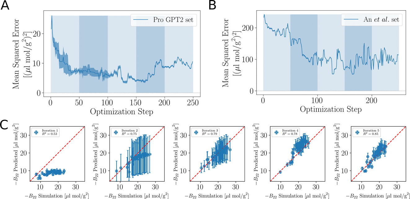

Fig. 2 Accuracy of the learned relationship between protein sequence and B₂₂. (A) Feedback between ML model and simulations. The shaded areas highlight the transitions between the sequences 0–50, 50–100, 100–150 and 150–200 in the first, second, and third iterations of the active learn procedure. The validation set is generated with ProtGPT2. (B) The same but with a validation set which includes more strongly interacting sequences from An et al. (C) Predicted B₂₂ from the active learning and computed from coarse-grained molecular dynamics. After the network was trained with N = 50 sequences. At the second iteration with a total of N = 100. Third iteration with N = 150 sequences (Fig. S1†).

When the model is interrogated for suggesting training examples, we also ask it to predict B₂₂ values for these sequences. After coarse-grained molecular dynamics simulations of these suggested sequences were performed, we compared how well those forecasts matched with the true values (Fig. 2C). This improvement is quantitatively reflected in the coefficient of determination (R²), which indicates how well the model predictions match the observed data. Initially, there is poor agreement between predicted and true estimates, indicated by R² = 0.53. The correlation between predicted and expected values continued to improve in the subsequent iterations as evidenced by the increasing R² values. By the fourth iteration, the R² value had risen to 0.85.

Note that a significantly longer calibration (e.g. 200 sequences instead of 50) in the initial training does not improve the overall outcome (see Fig. S1 in the ESI†). We tentatively conclude that results from the suggested sequences in active learning are more important, or that there is not much new information in these additional initial sequences.

As remarked previously, after just 50 such steps, when the model was interrogated to suggest the next batch of sequences to train with, it already picked up sequences with very negative B₂₂ values. When coarse-grained molecular dynamics simulations of these sequences were run, we found that the distribution of B₂₂ values had clearly shifted from a mean value of −2.3 μL mol⁻¹ g⁻² to −18.7 μL mol⁻¹ g⁻² (see iteration 1 in Fig. 3A). Subsequent iterations of training with examples requested by the model led to a further shift to even further negative values.

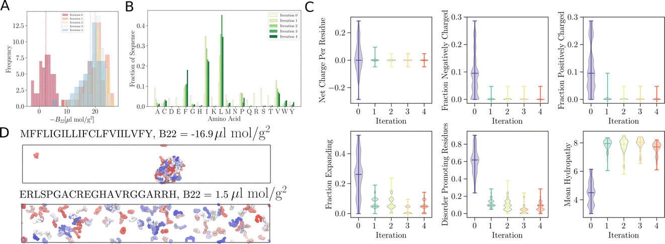Fig. 3 trained to maximise the −B₂₂ values, thereby suggesting interacting sequences. (A) Distribution of −B₂₂ after each iteration shifts towards more negative values. (B) The plot depicts the amino acid fractions in each iteration, showing a higher fraction of isoleucine (I), leucine (L), valine (V), and phenylalanine (F). (C) Analysis of the amino acid composition of the sequences suggested by the model after each iteration provides insight into the evolving composition of the optimised sequences. (D) Representative simulation snapshot of the protein sequences suggested by in the third iteration.

In addition to these quantitative metrics around B₂₂ values, in Fig. 3B we show that even the amino acid composition of the suggested sequences changed in biologically meaningful ways. The sequences get enriched with hydrophobic amino acids such as Ile, Leu, and Val. Charged residues are already lost in the first stage of learning. Impressively, all of these biologically and chemically sensible changes emerged without explicit input regarding information about the charge or hydrophobicity of the residues during training. We attribute this to the featurisation with the UniRep LSTM, and it illustrates the remarkable ability of the model to learn and capture relevant physicochemical properties from the sequence data alone. Many of the sequences we provided initially feature charged residues (Fig. 3C). While these sequences are not highly charged, with a net charge per residue close to 0, some sequences are enriched in positively or negatively charged residues. The model seems to learn from the input sequences that a simple way to enhance protein–protein chain interactions is to eliminate charged residues. It is important to note that complementary patches of positively and negatively charged residues can give rise to strong interactions and protein condensation via complex coacervation.^7,38 The input sequence set includes sequences which feature a third or half of the residues favouring expanded conformations. As the training progresses, the number of disorder promoting residues decreases strongly with iteration. At the same time the mean hydrophobicity of the suggested sequences increases.

We expect that sequences with large negative values of B₂₂ interact strongly and phase separate, which we verified by simulating multiple chains for a sequence from iteration 3 (Fig. 3D). Multiple chains of this peptide form a condensate as expected given its favourable inter-chain interactions. Conversely, for sequences with a positive B₂₂ we expect that the chains are not interacting with each other and that the chains prefer to stay separate from each other and do not phase separate as shown for a sequence from the validation data set (Fig. 3D). We note that the HPS model which underestimates interactions of Arg residues likely underestimates the self interactions of this peptide.

3.1.1 Influence of the force field in the coarse-grained simulations. To examine how the coarse-grained simulation model we use affects the suggested sequences, we conducted coarse-grained simulations using the CALVADOS2 force field,^13,39 which is a reparameterisation of HPS and more accurately describes the interactions of disordered proteins. We used the same initial set of sequences to calibrate. The distribution of −B₂₂ from the sequences suggested by training shifted towards larger values (Fig. 4A) of −B₂₂ of close to 0 μL mol⁻¹ g⁻² (iteration 0) to approximately 10 μL mol⁻¹ g⁻² (iteration 3). The sequences the model suggested are enriched with Tyr and Trp residues (Fig. 4B). Consistent with BO employing the HPS model, the fraction of disorder-promoting residues decreases across the iterations. However, in contrast to the HPS model, the mean hydropathy value of the suggested sequences decreases when using the CALVADOS force field (Fig. 4C).^13,39 This can be attributed to the increase in the fraction of tyrosine and tryptophan residues, which have a lower hydropathy index compared to isoleucine, leucine, valine, and phenylalanine, as reported in the Kyte–Doolittle hydropathy scale.⁴⁰

Fig. 4 Optimisation by maximising −B₂₂ values, where the simulations are conducted using the CALVADOS force field.¹³ (A) The distribution of B₂₂ values for 5 iterations of optimisation. The observed distribution shifts towards increasingly negative values compared with the HPS model, indicating a trend towards sequences with stronger interactions. (B) The plot illustrates the fraction of amino acids present in the sequences suggested by during each iteration of optimisation. Notably, there is a noticeable increase in the fraction of isoleucine (I), leucine (L), valine (V), and phenylalanine (F) over successive iterations. (C) Analysis of the amino acid compositions of the sequences suggested by the model after each iteration.

3.1.2 Sensitivity to acquisition function: test with expected improvement. From the previous discussion, we showed that active learning enabled us to very efficiently find strongly interacting sequences. However, the peptide sequences we suggested are likely to be hydrophobic for the actual realisation of peptide-based condensate material in a laboratory experiment. For the practical application of designing novel peptide-based condensate materials, one likely needs to perform multi-parameter optimisation to achieve a trade-off between protein interactions and fluidity²⁹ of the resulting materials, and change the acquisition function accordingly.

Therefore, to potentially identify alternative solutions while exploring the sequence space, we independently trained the model using sequences ranked best by the Expected Improvement (EI) acquisition function. The mean squared error (MSE) between the predicted and expected −B₂₂ of the ProteinGPT2 validation set, decreased with each training step (Fig. 5A), similar to what we observed in the UCB-based model. The model suggests sequences with diverse amino acid compositions (Fig. 5B). Examining the suggested sequences, we found that the EI-based optimisation found less strong interactors (smaller −B₂₂ values) compared to the model trained using the Upper Confidence Bound (UCB) acquisition function (Fig. S2†). The UCB-based optimisation predominantly predicted sequences with high negative B₂₂ values, while the EI-based model predicted a wider range of sequences, mostly with negative B₂₂ values and a small fraction with positive B₂₂ values.

Fig. 5 Optimisation using Expected Improvement (EI) acquisition function to find the optimal value of −B₂₂. (A) Evolution of mean squared error (MSE) between the predicted and expected −B₂₂ of the ProteinGPT2 validation set. (B) Fraction of amino acids in the sequences suggested by after each iteration. (C) Snapshot of the simulations of sequences suggested by at the 4th iteration. (D) The sequences with more negative B₂₂ showed clear phase separation (Fig. S2B†).

When we simulated the sequences suggested by the model in the 4th iteration, those with negative B₂₂ values in particularly exhibited clear phase separation—forming dense, condensed phases (see Fig. 5C and D). The phase-separating sequence not only features aromatic residues such as Trp and Phe and hydrophobic residues such as Val, but also negatively charged Asp and positively charged Arg at its C-terminal end. Interactions of positively and negatively charged amino acids can also contribute to phase separation,^38,41 provided the net charge of the sequence is low to moderate.³⁸ Overall the optimisation using UCB led to the identification of sequences with stronger interactions than EI. However, we note that, in the search for an optimal solution, UCB had led to less diverse sequence structures. On the other hand, the sequences ranked by EI were more diverse in amino acid composition but this came at the cost of not touching the sequence space of the most negative B₂₂ chains. These differences are evident in the distributions shown in Fig. S2.†

3.2 Designing peptides that do not interact

Employing the same approach, we can design peptides which do not interact with copies of themselves. For many biotechnological applications, one would want to minimise the interactions between proteins, e.g., to reduce the aggregation of therapeutic antibodies.⁴² Non-interacting sequences can be useful building blocks in protein design,⁹ for example when combining protein domains with different functionalities. To decrease the propensity for protein self-interaction, we maximise B₂₂ rather than −B₂₂, as previously done for promoting interactions.

As the BO proceeds, suggested sequences tend to have more positive B₂₂ values (Fig. 6A) than the initial set of sequences we have used to start the BO (referred to as “Iteration 0”). Interestingly, at the first iteration, the proposed sequences feature a combination of negatively charged amino acids, such as glutamic acid (Glu) and some aspartic acid (Asp) residues, as well as positively charged amino acids, including lysine (Lys) and arginine (Arg) (Fig. 6B and C). In the subsequent second, third and fourth iterations, Arg residues become highly enriched (Fig. 6B). Note that the enrichment in Arg residues may be partially due to the specific choices made in the parameterisation of the coarse-grained simulation model we employ. While Arg is positively charged and increasing the net positive or negative charge of a peptide can prevent phase separation,³⁸ Arg residues have a very low tendency to interact with other protein residues in the version of residue-level coarse-grained HPS model³⁴ we employ here. Tesei et al., have shown that a higher interaction strength of Arg for other amino acids leads to a better overall description of disorder proteins, their phase behaviour and properties.^13,39 The net charge per residue increases as the training progresses (Fig. 6C). Residues tend to favour extended rather than collapsed conformations. The fraction of negatively charged amino acids in the selected sequences becomes negligible after the first iteration (Fig. 6C). Concurrently, the fraction of amino acids associated with favouring extended rather than collapsed conformations increases compared to the initially input sequences. Analogously, the fraction of disorder promoting residues increases with each iteration. However, in the third iteration, there is a temporary drop in the fraction of disorder promoting residues, but this trend is reversed in the fourth iteration, where a high level of disorder-promoting residues is observed once again. Conversely, the mean hydrophobicity decreases as there are almost no aromatic residues (Phe, Tyr, and Trp) present in the sequences suggested by the active learning process.

Fig. 6 Design of non-interacting sequences using , by training to maximise +B₂₂ values, thereby suggesting sequences with minimal intermolecular interactions. (A) Distribution of B₂₂ values for the sequences suggested by after each iteration, showing a shift towards higher B₂₂ values, indicating the evolution of non-interacting sequences. (B) Amino acid composition of the suggested sequences, exhibiting an increasing fraction of the positively charged amino acid arginine (Arg) after each iteration. (C) Analysis of amino acid composition in the suggested sequences. The fraction of positively charged residues increases with each iteration, while the mean hydropathy decreases, reflecting the enrichment of charged residues. (D) Simulation conducted with the sequence suggested by after the 4th iteration. The simulation reveals that the suggested sequence does not undergo phase separation, remaining uniformly distributed throughout the simulation box.

To test whether these sequences actually interact with each other or not, we observed their behaviour in our CG simulations. In Fig. 6D, we show a snapshot of such a simulation of protein with B₂₂ = 4.0 μL mol g⁻². Clearly, the suggested sequence remains uniformly distributed throughout the simulation box, preferring to not interact with its identical chains and therefore not showing any sign of phase separation.

3.3 Designing peptides binding to phase-separated condensates

To investigate the ability of peptides to interact with pre-formed condensates, we initiated 70 simulations with peptides and a pre-formed condensate of the C-terminal domain of RNA Polymerase II (CTD).⁷

By optimising the peptide sequences to maximise the magnitude of the negative partition free energy (−ΔG), our active learning approach effectively identifies peptides with an enhanced propensity to interact with the condensed phase. Just like for the B₂₂ task, the performance of the model was evaluated using the mean squared error (MSE) calculated for a validation set of peptides. Remarkably, the MSE showed a significant decrease after just 50 training steps—similar to other tasks studied here—with MSE dropping from above 200 to less than 50 indicating that the model could effectively capture the underlying patterns and characteristics of the peptide-CTD condensate interactions. In the second iteration hydrophobic residues such as Cys, Phe, Leu, and Trp residues are very prominently enriched (Fig. 7C, S4A and B†). After four iterations of the Bayesian optimisation cycle, peptides are highly enriched in Trp residues. At this stage, peptides are uniformly distributed in the dense condensate phase. At the same time sampling the dilute concentration of the peptides becomes very challenging and long simulations are required for proper equilibration of the peptides between the dilute and condensate phases. Once the peptides are interacting strongly with the condensates and the dilute concentration becomes difficult to sample further, so enhancing the interactions of the peptides with the condensates becomes difficult. However, at this stage, the design task has in some sense been successfully completed as strongly interacting protein sequences have been found. We note that the lack of sequence diversity means that these peptides are likely too hydrophobic to be useful for biochemical and biotechnological applications, but our investigation shows that it is possible to quickly identify sequences which bind to condensates given a coarse-grained simulation model.

Fig. 7 Designing peptides which bind to a phase-separated condensate of CTD. (A) Grey CTD chains. Light blue peptide chains. (Top) Peptide weakly interacting with condensate. (Bottom) Peptide from BO, which interacts strongly. (B) Progress of the training by comparison to the validation data set. Each training step corresponds to an additional sequence and corresponding binding propensity being processed by . (C) Changes in the amino acid composition of sequences binding with ideal CTD condensate after each iteration. (D) For human CTD condensate. (E) AlphaFold (Q95XN0) structure of LIN65. The intrinsically disordered region is shown in pink, and the ordered regions, excluded from the analysis, are shown in grey. A 20-mer sequence from the disordered region is shown in blue. (F) Correlation plot of predicted and computed ΔG values for LIN-65 fragments and peptides suggested by in iteration 7.

We also performed iterative optimisation to identify sequences that bind effectively to human CTD condensates.⁴³ The human CTD (hCTD) sequence deviates from the ideal CTD sequence, which consists of a consensus repeat of heptad motifs. During the training process with ,²⁵ the algorithm suggested peptide sequences with a similar composition to the sequences found in the previous case, but featuring a higher fraction of the following amino acid residues: Trp, Phe, Leu, and Cys (Fig. 7D, S4C and D).†

Once trained, such a model can quickly evaluate many novel sequences for their potential to interact with specific condensates without requiring time-consuming simulations for each sequence. It can generalize from learned patterns to predict the interaction propensity of sequences different from those in the training set. For instance, we used the trained model to investigate interactions between LIN-65 and RNA Polymerase II (Pol II). In C. elegans, LIN-65 (Fig. 7E) is an important regulator of chromatin organisation by supporting the formation of heterochromatin which represses the transcription of genes. Given that the CTD of RNA Pol II is critical for transcription, but LIN-65 is associated with the repression of transcription, we surmised that disordered sequences in the LIN-65 disordered regions may be disfavoured from binding to CTD condensates and this preference encoded in the sequence of LIN-65 could contribute to its specificity in separating transcribed genes from heterochromatin. Since the model is trained on 20-mer sequences, we divided the intrinsically disordered region of LIN-65 into 20-mer fragments (Fig. 7E, pin and blue regions). We then predicted the propensity of LIN-65 fragments to be recruited to CTD condensates using the trained model. The correlation plots shown in Fig. 7F, indicate that the recruitment propensity of LIN-65 fragments is lower than that of sequences suggested by after the seventh iteration, as the ΔG is lower for LIN-65 fragments compared to the sequences suggested (Fig. S4E and F†). This predictive ability without new simulations showcases the powerful application of machine learning in studying protein–condensate interactions.

3.4 Design of multiphasic condensates

To explore the nature of sequences that can be recruited to CTD condensates while forming multiphasic structures, we employed a strategy based on the second virial coefficient (B₂₂). We calculated B₂₂ for a given sequence interacting with itself and with a 21-mer CTD sequence. The residue-level coarse-grained HPS force field we employ for these simulations captures the interactions of 21-mer CTD sequences well, as established through comparisons to all-atom simulations with explicit solvent.⁷ The fitness function, ΔB₂₂ = −B₂₂[seq–seq] + B₂₂[seq–ctd], was optimised using , aiming to identify sequences that interact more strongly with sequences of the same type than with CTD. Through this optimisation process, suggested highly hydrophobic sequences that exhibited stronger interactions with themselves compared to their interactions with the CTD sequence (Fig. 8 and S3).† To validate the formation of multiphasic condensates, we conducted simulations with a system comprising 300 chains of the 21-mer CTD sequence and 300 chains of the highly hydrophobic sequences suggested by (Fig. 8B and C). Analysis of the density profiles from these simulations revealed a distinct phase separation, where the highly hydrophobic sequences formed the core of the condensate, while the comparatively less hydrophobic CTD sequences formed a surrounding shell (Fig. 8C–F). For lower ΔB₂₂ values, the density profile shows a mixed condensate(Fig. 8G–I). This observation suggests that the highly hydrophobic sequences identified through the optimisation process have the propensity to be recruited to CTD condensates while maintaining a distinct phase separation, leading to the formation of a multiphasic condensate structure with a hydrophobic core and a CTD-rich shell.

Fig. 8 Designing multiphasic condensates using . (A) Amino acid composition of the sequences suggested by after each iteration of optimising the fitness function. (B) Simulation with 300 chains each of the optimised sequence and CTD, illustrating the formation of a mixed condensate when the B₂₂ values of sequence–sequence and sequence–CTD interactions are comparable. The corresponding density profile is shown in (G). (C) Formation of a remixed phase when B₂₂ of the sequence–sequence is notably lower than sequence–CTD. The corresponding density profile is shown in (D). (D–F) Density profile showing the formation of multiphasic condensate when the ΔB₂₂ is higher, indicating stronger sequence–sequence interactions compared to sequence–CTD interactions. (G–I) Density profile in the case of mixed phase condensate formed when the ΔB₂₂ is lower, suggesting weaker sequence–sequence interactions relative to sequence–CTD interactions.

4 Conclusions

While modelling sequence–property relationships remains a difficult challenge, here we showed it is possible to train neural network models with molecular dynamics simulations to design disordered proteins to: (1) self-interact and phase separate and (2) to bind to phase separated condensates and (3) even shape the morphologies of phase-separated condensates. For this we employed the approach developed by Yang et al.²⁵ that utilises appropriate featurisation from pre-trained sequence models,^24,25,44 and Bayesian Optimisation (BO) for sampling the candidates most useful for training and protein design (Fig. 1). For these design tasks a limited number of sequences, with numeric labels from molecular dynamics, are sufficient, e.g., 50–100 sequences with labels are enough to predict B₂₂ with reasonable accuracy (Fig. 2C). Even when no explicit information about the hydrophobicity and charge of individual amino acids is given,²⁰ approaches based on pre-trained language models are able to learn biologically and chemically relevant information from the sequence data alone.

Active learning provides a significant advantage when individual computations are expensive and an efficient way of traversing a large parameter space is needed. While training and optimising for certain fitness criteria, one must appropriately tune the balance between exploration and exploitation. The improvement using CALVADOS force-field^13,39 highlighted the importance of the availability of state-of-the-art molecular force fields. The sequences identified from the coarse-grained simulations could be further explored with atomistic resolution along with explicit solvent, to include the role of water, ions and secondary structure formation and provide further insight into the molecular driving forces.³⁰

A key limitation of the present work is that many of the peptides we suggest here may be too hydrophobic to be realised in a laboratory experiment. Recent work shows that one could explicitly consider the synthesizability of peptides in a neural network.⁴⁵ As pointed out by An et al.,²⁹ optimising interaction strength comes with a trade-off in terms of transport properties of the material and considering this in multi-parameter optimisation will yield protein sequences that are more balanced with regards to hydrophobic and non-hydrophobic residues. While we have not attempted to perform multi-parameter optimisation, for future practical applications to inform the design of novel materials underpinned by protein phase separation, multi-parameter optimisation is likely beneficial.

Data availability

All codes and datasets related to this study can be accessed at the following GitHub repository: https://github.com/cartilage-ftw/active-learning.

Author contributions

A. C. S. designed and ran most of the HOOMD simulations. A. A. implemented the active learning workflow with the MD simulations. V. X. provided the protein sequences used for training. A. C. S., A. A., J. P. and L. S. conceived the study and interpreted the data. L. S. oversaw the study. A. C. S., A. A. and L. S. wrote the manuscript.

Conflicts of interest

There are no conflicts to declare.

Acknowledgements

A. C. S. and L. S. S. thank M³ODEL for support. L. S. S. acknowledges support by ReALity (Resilience, Adaptation and Longevity) and Forschungsinitiative des Landes Rheinland-Pfalz. This project was funded by SFB 1551 Project No. 464588647 of the DFG (Deutsche Forschungsgemeinschaft). We acknowledge a mini grant from the Emergent AI (EAI) Center of Carl Zeiss Foundation. L. S. S. and A. A. thank the Deutsche Forschungsgemeinschaft (DFG, German Research Foundation) – Project number 233630050 – TRR 146 for support. We gratefully acknowledge the advisory services offered and the computing time granted on the supercomputers Mogon II at Johannes Gutenberg University Mainz, which is a member of the AHRP (Alliance for High Performance Computing in Rhineland Palatinate) and the Gauss Alliance e.V. We thank Dr Noelia Ferruz, Prof. Dr Susanne Gerber, Yehor Tuchkov, Prof. Dr Heinz Koeppl, Dr Sören von Bülow and Prof. Dr Shikha Dhiman for inspiring discussions.

Notes and references

1. E. W. Martin, A. S. Holehouse, I. Peran, M. Farag, J. J. Incicco, A. Bremer, C. R. Grace, A. Soranno, R. V. Pappu and T. Mittag, Science, 2020, 367, 694–699.
2. B. Tsang, I. Pritišanac, S. W. Scherer, A. M. Moses and J. D. Forman-Kay, Cell, 2020, 183, 1742–1756.
3. A. Zbinden, M. Pérez-Berlanga, P. De Rossi and M. Polymenidou, Dev. Cell, 2020, 55, 45–68.
4. L. A. Gruijs da Silva, F. Simonetti, S. Hutten, H. Riemenschneider, E. L. Sternburg, L. M. Pietrek, J. Gebel, V. Dötsch, D. Edbauer, G. Hummer, L. S. Stelzl and D. Dormann, EMBO J., 2022, 41, e108443.
5. R. M. Welles, K. A. Sojitra, M. V. Garabedian, B. Xia, W. Wang, M. Guan, R. M. Regy, E. R. Gallagher, D. A. Hammer, J. Mittal and M. C. Good, Nat. Chem., 2024, 16, 1062–1072.
6. M. Farag, W. M. Borcherds, A. Bremer, T. Mittag and R. V. Pappu, Nat. Commun., 2023, 14, 5527.
7. A. Changiarath, J. J. Michels, R. H. Rodriguez, S. M. Hanson, F. Schmid, J. Padeken and L. S. Stelzl, bioRxiv, 2024, preprint,  DOI:10.1101/2024.03.16.585180.
8. M. Dzuricky, B. A. Rogers, A. Shahid, P. S. Cremer and A. Chilkoti, Nat. Chem., 2020, 12, 814–825.
9. A. Gräwe, M. Merkx and V. Stein, Bioconjugate Chem., 2022, 33, 1415–1421.
10. S. Rekhi, C. G. Garcia, M. Barai, A. Rizuan, B. S. Schuster, K. L. Kiick and J. Mittal, Nat. Chem., 2024, 16, 1113–1124.
11. J. A. Joseph, A. Reinhardt, A. Aguirre, P. Y. Chew, K. O. Russell, J. R. Espinosa, A. Garaizar and R. Collepardo-Guevara, Nat. Comput. Sci., 2021, 1, 732–743.
12. W. M. Jacobs, J. Chem. Theory Comput., 2023, 19, 3429–3445.
13. G. Tesei and K. Lindorff-Larsen, Open Research Europe, 2023, 2, 94.
14. G. M. Ginell, R. J. Emenecker, J. M. Lotthammer, E. T. Usher and A. S. Holehouse, bioRxiv, 2024, preprint,  DOI:10.1101/2024.06.03.597104.
15. S. von Bülow, G. Tesei and K. Lindorff-Larsen, bioRxiv, 2024, preprint,  DOI:10.1101/2024.06.03.597109.
16. F. Pesce, A. Bremer, G. Tesei, J. B. Hopkins, C. R. Grace, T. Mittag and K. Lindorff-Larsen, Sci. Adv., 2024, 10(35), eadm9926,  DOI:10.1126/sciadv.adm9926.
17. T. Hoffbauer and B. Strodel, bioRxiv, 2024, preprint,  DOI:10.1101/2024.01.12.575432.
18. X. Zeng, C. Liu, M. J. Fossat, P. Ren, A. Chilkoti and R. V. Pappu, APL Mater., 2021, 9, 021119.
19. P. Y. Chew, J. A. Joseph, R. Collepardo-Guevara and A. Reinhardt, Chem. Sci., 2023, 14, 1820–1836.
20. A. Elnaggar, M. Heinzinger, C. Dallago, G. Rehawi, Y. Wang, L. Jones, T. Gibbs, T. Feher, C. Angerer, M. Steinegger, D. Bhowmik and B. Rost, IEEE Trans. Pattern Anal. Mach. Intell., 2022, 44, 7112–7127.
21. N. Brandes, D. Ofer, Y. Peleg, N. Rappoport and M. Linial, Bioinformatics, 2022, 38, 2102–2110.
22. R. Verkuil, O. Kabeli, Y. Du, B. I. M. Wicky, L. F. Milles, J. Dauparas, D. Baker, S. Ovchinnikov, T. Sercu and A. Rives, bioRxiv, 2022, preprint,  DOI:10.1101/2022.12.21.521521.
23. N. Ferruz, S. Schmidt and B. Höcker, Nat. Commun., 2022, 13, 4348.
24. E. C. Alley, G. Khimulya, S. Biswas, M. AlQuraishi and G. M. Church, Nat. Methods, 2019, 16, 1315–1322.
25. Z. Yang, K. A. Milas and A. D. White, bioRxiv, 2022, preprint, https://doi.org/10.1101/2022.08.05.502972.
26. E. J. Ma and A. Kummer, bioRxiv, 2020, preprint,  DOI:10.1101/2020.05.11.088344.
27. M. Aldeghi and C. W. Coley, Chem. Sci., 2022, 13, 8221–8223.
28. K. Shmilovich, S. S. Panda, A. Stouffer, J. D. Tovar and A. L. Ferguson, Digital Discovery, 2022, 1, 448–462.
29. Y. An, M. A. Webb and W. M. Jacobs, Sci. Adv., 2024, 10, eadj2448.
30. B. Mohr, K. Shmilovich, I. S. Kleinwächter, D. Schneider, A. L. Ferguson and T. Bereau, Chem. Sci., 2022, 13, 4498–4511.
31. Y. Khalak, G. Tresadern, D. F. Hahn, B. L. de Groot and V. Gapsys, J. Chem. Theory Comput., 2022, 18, 6259–6270.
32. B. Lakshminarayanan, A. Pritzel and C. Blundell, in NIPS’17: Proceedings of the 31st International Conference on Neural Information Processing Systems, Curran Associates Inc., Red Hook, NY, USA, 2017, pp. 6405–6416.
33. P. I. Frazier, arXiv, preprint, arXiv:1807.02811, 2018,  DOI:10.48550/arXiv.1807.02811.
34. G. L. Dignon, W. Zheng, Y. C. Kim, R. B. Best and J. Mittal, PLoS Comput. Biol., 2018, 14, e1005941–23.
35. J. A. Anderson, J. Glaser and S. C. Glotzer, Comput. Mater. Sci., 2020, 173, 109363.
36. J. A. Riback, L. Zhu, M. C. Ferrolino, M. Tolbert, D. M. Mitrea, D. W. Sanders, M.-T. Wei, R. W. Kriwacki and C. P. Brangwynne, Nature, 2020, 581, 209–214.
37. A. S. Holehouse, R. K. Das, J. N. Ahad, M. O. G. Richardson and R. V. Pappu, Biophys. J., 2017, 112, 16–21.
38. A. Bremer, M. Farag, W. M. Borcherds, I. Peran, E. W. Martin, R. V. Pappu and T. Mittag, Nat. Chem., 2022, 14, 196–207.
39. G. Tesei, T. K. Schulze, R. Crehuet and K. Lindorff-Larsen, Proc. Natl. Acad. Sci. U. S. A., 2021, 118(44), e2111696118.
40. J. Kyte and R. F. Doolittle, J. Mol. Biol., 1982, 157, 105–132.
41. D. J. Bauer, L. S. Stelzl and A. Nikoubashman, J. Chem. Phys., 2022, 157, 154903.
42. T. M. Prass, P. Garidel, M. Blech and L. V. Schäfer, J. Chem. Inf. Model., 2023, 63, 6129–6140.
43. D. Flores-Solis, I. P. Lushpinskaia, A. A. Polyansky, A. Changiarath, M. Boehning, M. Mirkovic, J. Walshe, L. M. Pietrek, P. Cramer, L. S. Stelzl, B. Zagrovic and M. Zweckstetter, Nat. Commun., 2023, 14, 5979.
44. Z. Lin, H. Akin, R. Rao, B. Hie, Z. Zhu, W. Lu, N. Smetanin, R. Verkuil, O. Kabeli, Y. Shmueli, A. dos Santos Costa, M. Fazel-Zarandi, T. Sercu, S. Candido and A. Rives, Science, 2023, 379, 1123–1130.
45. R. Zhang, H. Wu, Y. Xiu, K. Li, N. Chen, Y. Wang, Y. Wang, X. Gao and F. Zhou, arXiv, preprint, arXiv:1807.02811, 2023,  DOI:10.48550/arXiv.1807.02811.

---

Footnote

† Electronic supplementary information (ESI) available. See DOI: https://doi.org/10.1039/d4fd00099d

---